Application of Non-Destructive Techniques on a Varve Sediment Record from Vouliagmeni Coastal Lake, Eastern Gulf of Corinth, Greece

 , , , and
Abstract
:1. Introduction
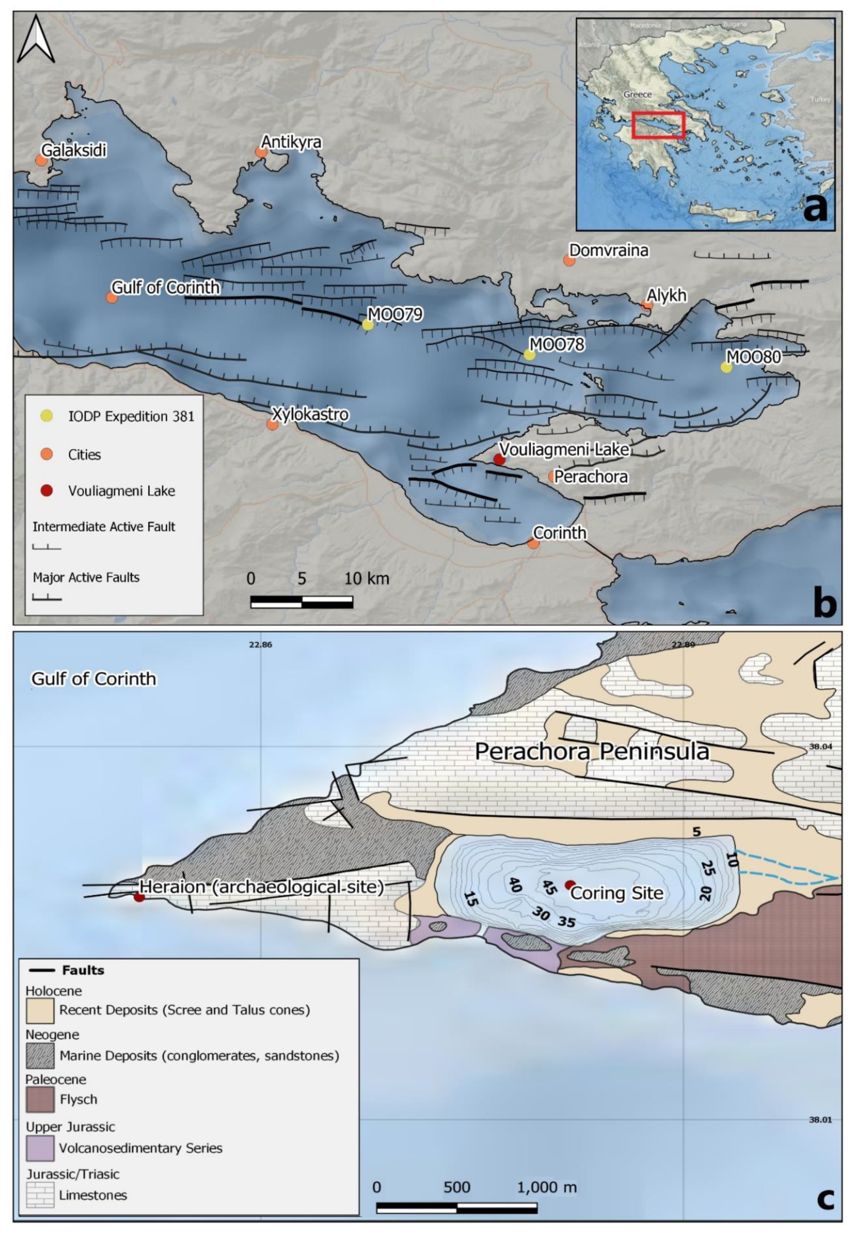
2. Study Area
3. Materials and Methods
3.1. Core Sampling
3.2. Sedimentology/Mineralogy
3.3. CT Scanning/Thin Sections
3.4. Elemental Composition
3.5. CT Scan Workflow
3.6. Core Chronology
4. Results
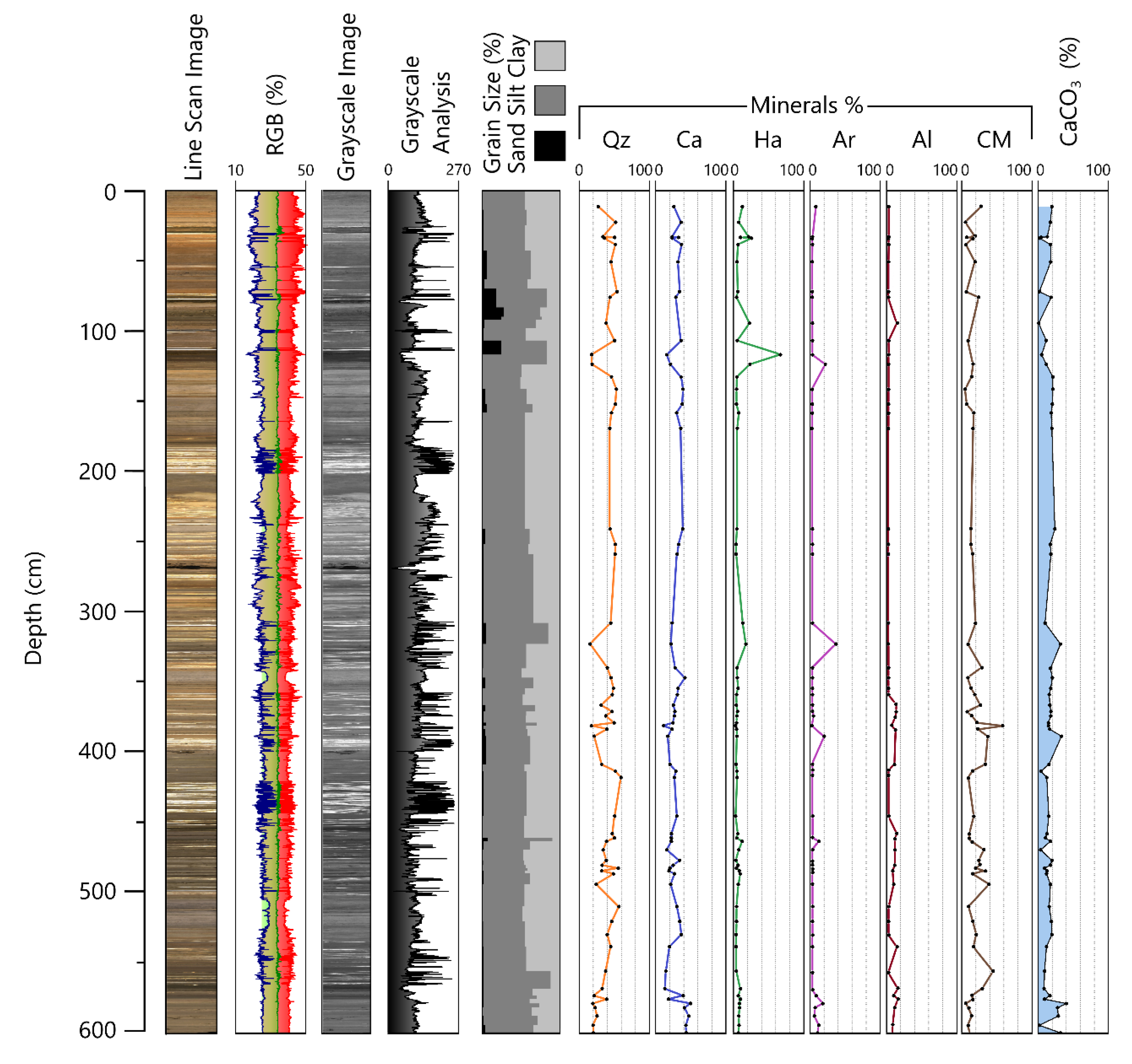
4.1. Core Description
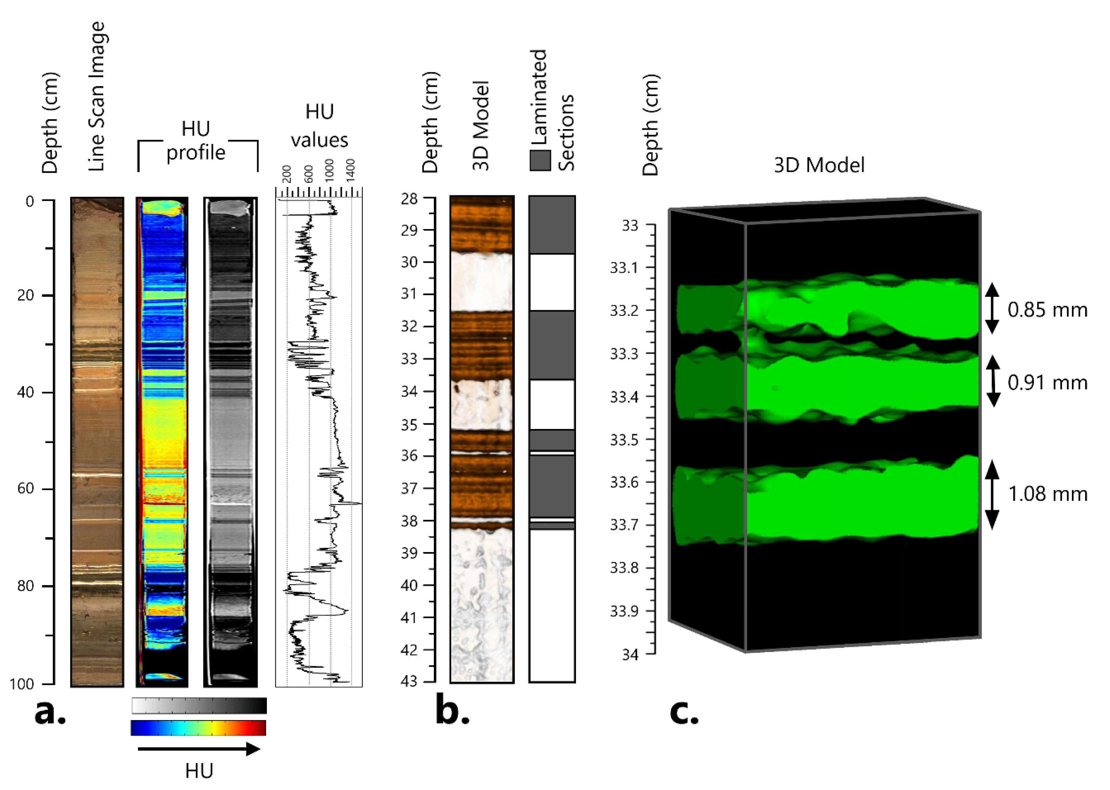
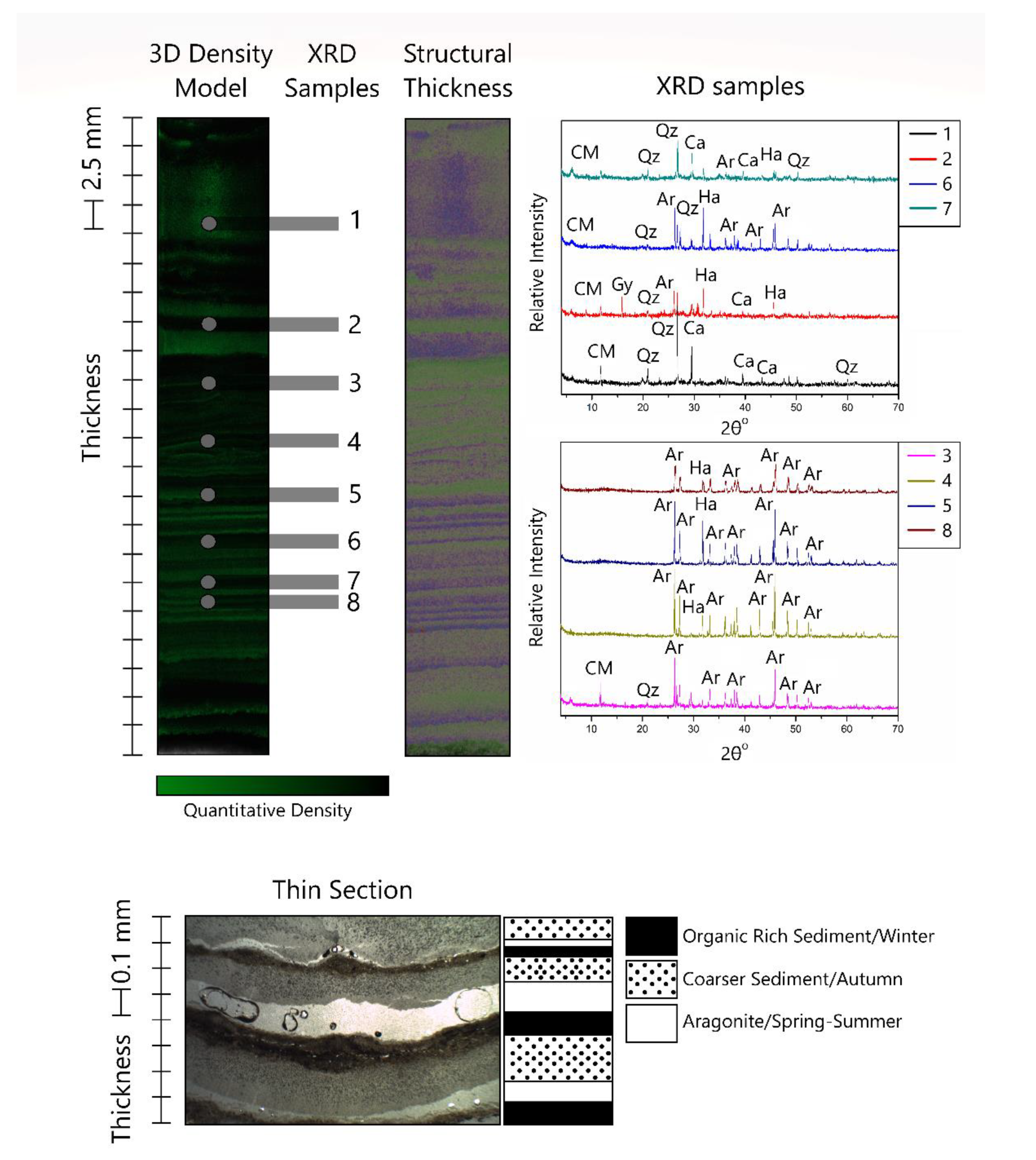
4.2. Microstructural Analysis
4.2.1. Laminated Sections
4.2.2. Non-Laminated Sections
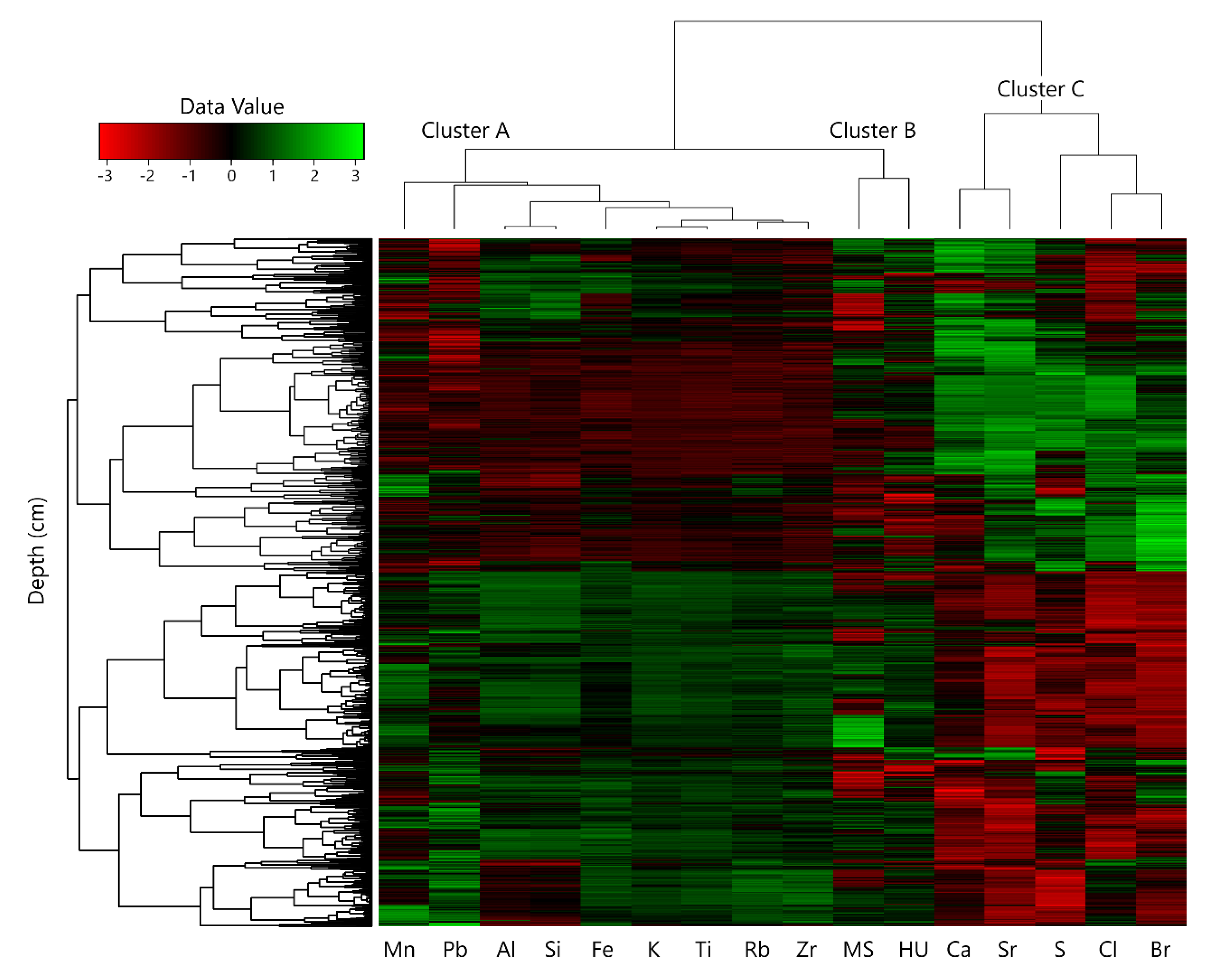
4.3. Hierarchical Clustering
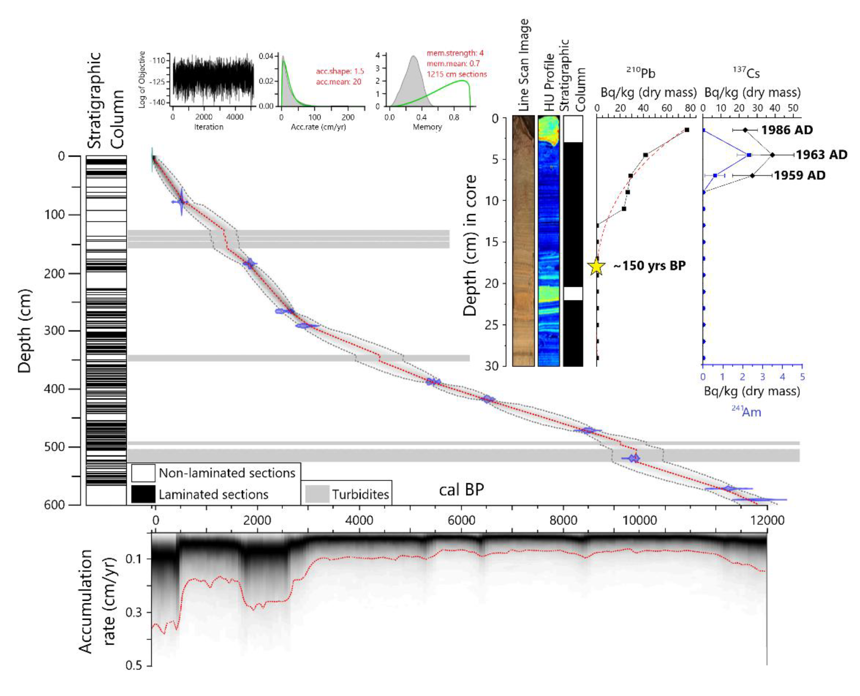
4.4. Bayesian Age-Depth Model
5. Discussion
5.1. Non-Destructive Proxies
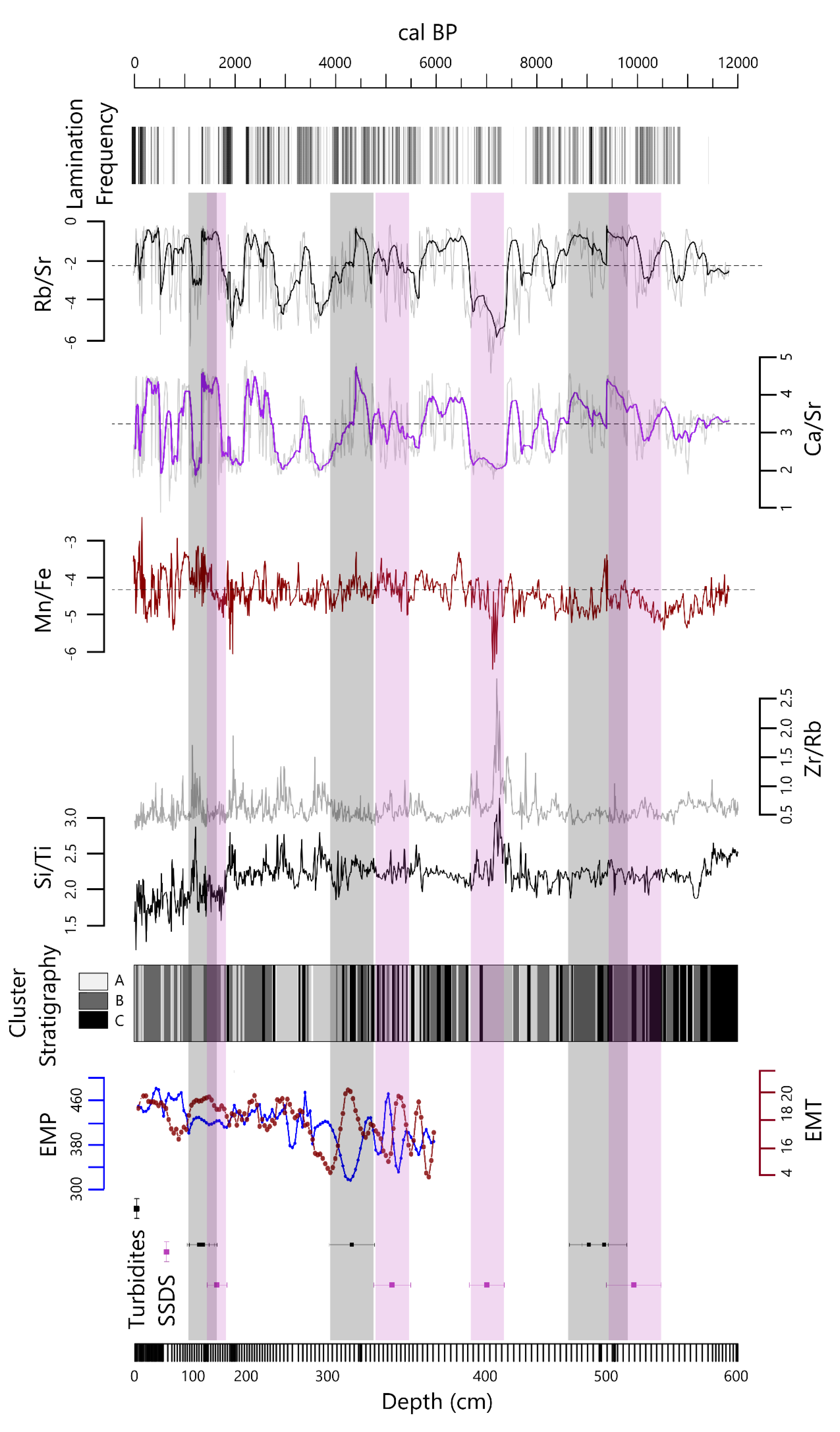
5.2. Paleoenvironmental Interpretation
6. Conclusions
Author Contributions
Funding
Acknowledgments
Conflicts of Interest
References
- Willis, K.J. The late Quaternary vegetational history of northwest Greece: I. Lake Gramousti. New Phytol. 1992, 121, 101–117. [Google Scholar] [CrossRef]
- Frogley, M.R.; Griffiths, H.I.; Heaton, T.H.E. Historical biogeography and late Quaternary environmental change of Lake Pamvotis, Ioannina (North-western Greece): Evidence from ostracods. J. Biogeogr. 2001, 28, 745–756. [Google Scholar] [CrossRef]
- Lawson, I.T.; Al-Omari, S.; Tzedakis, P.C.; Bryant, C.L.; Christanis, K. Lateglacial and Holocene vegetation history at Nisi Fen and the Boras mountains, northern Greece. Holocene 2005, 15, 873–887. [Google Scholar] [CrossRef]
- Leng, M.J.; Baneschi, I.; Zanchetta, G.; Jex, C.N.; Wagner, B.; Vogel, H. Late Quaternary palaeoenvironmental reconstruction from Lakes Ohrid and Prespa (Macedonia/Albania border) using stable isotopes. Biogeosciences 2010, 7, 3109–3122. [Google Scholar] [CrossRef] [Green Version]
- Ariztegui, D.; Anselmetti, F.S.; Robbiani, J.M.; Bernasconi, S.M.; Brati, E.; Gilli, A.; Lehmann, M.F. Natural and human-induced environmental change in southern Albania for the last 300 years—Constraints from the Lake Butrint sedimentary record. Glob. Planet. Chang. 2010, 71, 183–192. [Google Scholar] [CrossRef] [Green Version]
- Francke, A.; Wagner, B.; Leng, M.J.; Rethemeyer, J. A late glacial to holocene record of environmental change from Lake Dojran (Macedonia, Greece). Clim. Past 2013, 9, 481–498. [Google Scholar] [CrossRef] [Green Version]
- Roberts, N. The Holocene: An Environmental History; John Wiley & Sons: New York, NY, USA, 2014. [Google Scholar]
- Lacey, J.H.; Francke, A.; Leng, M.J.; Vane, C.H.; Wagner, B. A high-resolution Late Glacial to Holocene record of environmental change in the Mediterranean from Lake Ohrid (Macedonia/Albania). Int. J. Earth Sci. 2015, 104, 1623–1638. [Google Scholar] [CrossRef] [Green Version]
- Seguin, J.; Avramidis, P.; Dörfler, W.; Emmanouilidis, A.; Unkel, I. A 2600-year high-resolution climate record from Lake Trichonida (SW Greece). E&G Quat. Sci. J. 2020, 69, 139–160. [Google Scholar] [CrossRef]
- Seguin, J.; Avramidis, P.; Haug, A.; Kessler, T.; Schimmelmann, A.; Unkel, I. Reconstruction of palaeoenvironmental variability based on an inter-comparison of four lacustrine archives on the Peloponnese (Greece) for the last 5000 years. E&G Quat. Sci. J. 2020, 69, 165–186. [Google Scholar] [CrossRef]
- Gassner, S.; Gobet, E.; Schwörer, C.; van Leeuwen, J.; Vogel, H.; Giagkoulis, T.; Makri, S.; Grosjean, M.; Panajiotidis, S.; Hafner, A.; et al. 20,000 years of interactions between climate, vegetation and land use in Northern Greece. Veg. Hist. Archaeobot. 2020, 29, 75–90. [Google Scholar] [CrossRef]
- Jahns, S. The Holocene history of vegetation and settlement at the coastal site of Lake Voulkaria in Acarnania, western Greece. Veg. Hist. Archaeobot. 2005, 14, 55–66. [Google Scholar] [CrossRef]
- Kuhnt, T.; Schmiedl, G.; Ehrmann, W.; Hamann, Y.; Andersen, N. Stable isotopic composition of Holocene benthic foraminifers from the Eastern Mediterranean Sea: Past changes in productivity and deep water oxygenation. Palaeogeogr. Palaeoclimatol. Palaeoecol. 2008, 268, 106–115. [Google Scholar] [CrossRef]
- Avramidis, P.; Iliopoulos, G.; Nikolaou, K.; Kontopoulos, N.; Koutsodendris, A.; van Wijngaarden, G.J. Holocene sedimentology and coastal geomorphology of Zakynthos Island, Ionian Sea: A history of a divided Mediterranean island. Palaeogeogr. Palaeoclimatol. Palaeoecol. 2017, 487, 340–354. [Google Scholar] [CrossRef]
- Norström, E.; Katrantsiotis, C.; Finné, M.; Risberg, J.; Smittenberg, R.H.; Bjursäter, S. Biomarker hydrogen isotope composition (δD) as proxy for Holocene hydroclimatic change and seismic activity in SW Peloponnese, Greece. J. Quat. Sci. 2018, 33, 563–574. [Google Scholar] [CrossRef]
- Emmanouilidis, A.; Katrantsiotis, C.; Norström, E.; Risberg, J.; Kylander, M.; Sheik, T.A.; Iliopoulos, G.; Avramidis, P. Middle to late Holocene palaeoenvironmental study of Gialova Lagoon, SW Peloponnese, Greece. Quat. Int. 2018, 476, 46–62. [Google Scholar] [CrossRef]
- Katrantsiotis, C.; Norström, E.; Smittenberg, R.H.; Finne, M.; Weiberg, E.; Hättestrand, M.; Avramidis, P.; Wastegård, S. Climate changes in the Eastern Mediterranean over the last 5000years and their links to the high-latitude atmospheric patterns and Asian monsoons. Glob. Planet. Chang. 2019, 175, 36–51. [Google Scholar] [CrossRef]
- Zolitschka, B.; Francus, P.; Ojala, A.E.K.; Schimmelmann, A. Varves in lake sediments—A review. Quat. Sci. Rev. 2015, 117, 1–41. [Google Scholar] [CrossRef]
- Schimmelmann, A.; Lange, C.B.; Schieber, J.; Francus, P.; Ojala, A.E.K.; Zolitschka, B. Varves in marine sediments: A review. Earth Sci. Rev. 2016, 159, 215–246. [Google Scholar] [CrossRef]
- Tylmann, W.; Zolitschka, B. Annually laminated lake sediments—Recent progress. Quaternary 2020, 3, 5. [Google Scholar] [CrossRef] [Green Version]
- Johansson, M.; Saarni, S.; Sorvari, J. Ultra-high-resolution monitoring of the catchment response to changing weather conditions using online sediment trapping. Quaternary 2019, 2, 18. [Google Scholar] [CrossRef] [Green Version]
- Salminen, S.; Saarni, S.; Tammelin, M.; Fukumoto, Y.; Saarinen, T. Varve distribution reveals spatiotemporal hypolimnetic hypoxia oscillations during the past 200 years in Lake Lehmilampi, eastern Finland. Quaternary 2019, 2, 20. [Google Scholar] [CrossRef] [Green Version]
- Theuerkauf, M.; Engelbrecht, E.; Dräger, N.; Hupfer, M.; Mrotzek, A.; Prager, A.; Scharnweber, T. Using annual resolution pollen analysis to synchronize varve and tree-ring records. Quaternary 2019, 2, 23. [Google Scholar] [CrossRef] [Green Version]
- Thys, S.; Van Daele, M.; Praet, N.; Jensen, B.; Van Dyck, T.; Haeussler, P.; Vandekerkhove, E.; Cnudde, V.; De Batist, M. Dropstones in lacustrine sediments as a record of snow avalanches—A validation of the proxy by combining satellite imagery and varve chronology at Kenai Lake (South-Central Alaska). Quaternary 2019, 2, 11. [Google Scholar] [CrossRef] [Green Version]
- Żarczyński, M.; Szmańda, J.; Tylmann, W. Grain-size distribution and structural characteristics of varved sediments from Lake Żabińskie (Northeastern Poland). Quaternary 2019, 2, 8. [Google Scholar] [CrossRef] [Green Version]
- Vegas-Vilarrúbia, T.; Rull, V.; Trapote, M.D.; Cao, M.; Rosell-Melé, A.; Buchaca, T.; Gomà, J.; López, P.; Sigró, J.; Safont, E.; et al. Modern analogue approach applied to high-resolution varved sediments—A synthesis for Lake Montcortès (Central Pyrenees). Quaternary 2020, 3, 1. [Google Scholar] [CrossRef] [Green Version]
- Hughen, K.; Southon, J.; Lehman, S.; Bertrand, C.; Turnbull, J. Updated Cariaco Basin 14 C calibration and activity record for the past 50,000 years. Quat. Sci. Rev. 2006, 25, 3216–3227. [Google Scholar] [CrossRef] [Green Version]
- Lauterbach, S.; Brauer, A.; Andersen, N.; Danielopol, D.; Dulski, P.; Huels, M.; Milecka, K.; Namiotko, T.; Obremska, M.; Von Grafenstein, U.; et al. Environmental responses to Lateglacial climatic fluctuations recorded in the sediments of pre-Alpine Lake Mondsee (northeastern Alps). J. Quat. Sci. 2011, 26, 253–267. [Google Scholar] [CrossRef] [Green Version]
- Corella, J.; Valero-Garcés, B.; Vicente-Serrano, S.; Brauer, A.; Benito, G. Three millennia of heavy rainfalls in Western Mediterranean: Frequency, seasonality and atmospheric drivers. Sci. Rep. 2016, 6, 38206. [Google Scholar] [CrossRef] [Green Version]
- Schlolaut, G.; Staff, R.; Brauer, A.; Lamb, H.; Marshall, M.; Ramsey, C.; Nakagawa, T. An extended and revised Lake Suigetsu varve chronology from ~50 to ~10 ka BP based on detailed sediment micro-facies analyses. Quat. Sci. Rev. 2018, 200, 351–366. [Google Scholar] [CrossRef] [Green Version]
- Vött, A.; Schriever, A.; Handl, M.; Brücker, H. Holocene Palaeographies of the easter Acheloos River Delta and the lagoon of Etoliko (NW Greece). J. Coast. Res. 2007, 234, 1042–1066. [Google Scholar] [CrossRef]
- Haenssler, E.; Nadeau, M.J.; Vött, A.; Unkel, I. Natural and human induced environmental changes preserved in a Holocene sediment sequence from the Etoliko Lagoon, Greece: New evidence from geochemical proxies. Quat. Int. 2013, 308–309, 89–104. [Google Scholar] [CrossRef]
- Koutsodendris, A.; Brauer, A.; Zacharias, I.; Putyrskaya, V.; Klemt, E.; Sangiorgi, F.; Pross, J. Ecosystem response to human- and climate-induced environmental stress on an anoxic coastal lagoon (Etoliko, Greece) since 1930 AD. J. Paleolimnol. 2015. [Google Scholar] [CrossRef]
- Koutsodendris, A.; Brauer, A.; Reed, J.; Plessen, B.; Friedrich, O.; Hennrich, B.; Zacharias, I.; Pross, J. Climate variability in SE Europe since 1450 AD based on a varved sediment record from Etoliko Lagoon (Western Greece). Quat. Sci. Rev. 2017. [Google Scholar] [CrossRef]
- Jansen, F.; Gaast, S.; Koster, B.; Vaars, A. CORTEX, a shipboard XRF-scanner for element analyses in split sediment cores. Mar. Geol. 1998, 151, 143–153. [Google Scholar] [CrossRef]
- Tjallingii, R.; Röhl, U.; Koelling, M.; Bickert, T. Influence of the water content on X-ray fluorescence core-scanning measurements in soft marine sediments. Geochem. Geophys. Geosyst. 2007. [Google Scholar] [CrossRef]
- Croudace, I.; Rindby, A.; ROTHWELL, R. ITRAX: Description and evaluation of a new multi-function X-ray core scanner. Geol. Soc. Lond. Spec. Publ. 2006, 267, 51–63. [Google Scholar] [CrossRef] [Green Version]
- Unkel, I.; Björck, S.; Wohlfarth, B. Deglacial environmental changes on Isla de los Estados (54.4° S), southeastern Tierra del Fuego. Quat. Sci. Rev. 2008, 27, 1541–1554. [Google Scholar] [CrossRef]
- Heimhoffer, U.; Ariztegui, D.; Lenniger, M.; Hesselbo, S.P.; Martill, D.M.; Rios-Netto, A. Decipering the depositional environment of the laminated Crato fossil beds (Early Cretaceous, Araripe Basin, North-eastern Brazil). Sedimentology 2010, 57, 677–694. [Google Scholar] [CrossRef]
- Kylander, M.E.; Ampel, L.; Wohlfarth, B.; Veres, D. High-resolution X-ray fluorescence core scanning analysis of Les Echets (France) sedimentary sequence: New insights from chemical proxies. J. Quat. Sci. 2011, 26, 109–117. [Google Scholar] [CrossRef]
- Deplazes, G.; Meckler, A.N.; Peterson, L.C.; Hamann, Y.; Aeschlimann, B.; Gunther, D.; Martinez-Garcia, A.; Haug, G. Fingerprint of tropical climate variability and sea level in sediments of the Cariaco Basin during the last glacial period. Sedimentology 2019, 66, 1967–1988. [Google Scholar] [CrossRef]
- Ketcham, R.; Carlson, W. Acquisition, optimization and interpretation of X-ray computed tomographic imagery: Applications to the geosciences. Comput. Geosci. 2001, 27, 381–400. [Google Scholar] [CrossRef]
- Rosenberg, R.; Davey, E.; Gunnarsson, J.; Norling, K.; Frank, M. Application of computer-aided tomography to visualize and quantify biogenic structures in marine sediment. Mar. Ecol. Prog. Ser. 2007. [Google Scholar] [CrossRef]
- St-Onge, G.; Long, B. CAT-scan analysis of sedimentary sequences: An ultrahigh-resolution paleoclimatic tool. Eng. Geol. 2008. [Google Scholar] [CrossRef]
- Bendle, J.; Palmer, A.; Carr, S. A comparison of micro-CT and thin section analysis of Lateglacial glaciolacustrine varves from Glen Roy, Scotland. Quat. Sci. Rev. 2015. [Google Scholar] [CrossRef]
- Vandorpe, T.; Collart, T.; Cnudde, V.; Lebreiro, S.; Hernández-Molina, F.J.; Alonso, B.; Mena, A.; Antón, L.; Van Rooij, D. Quantitative characterisation of contourite deposits using medical CT. Mar. Geol. 2019, 417, 106003. [Google Scholar] [CrossRef]
- Tanaka, A.; Nakano, T.; Ikehara, K. X-ray computerized tomography analysis and density estimation using a sediment core from the Challenger Mound area in the Porcupine Seabight, off Western Ireland. Earth Planets Sp. 2011, 63, 103–110. [Google Scholar] [CrossRef] [Green Version]
- Polacci, M.; Baker, D.; Mancini, L.; Tromba, G.; Zanini, F. Three-dimensional investigation of volcanic textures by X-ray microtomography and implications for conduit processes. Geophys. Res. Lett. 2006. [Google Scholar] [CrossRef] [Green Version]
- Sleutel, S.; Cnudde, V.; Masschaele, B.; Vlassenbroek, J.; Dierick, M.; Hoorebeke, L.; Jacobs, P.; De Neve, S. Comparison of different nano- and micro-focus X-ray computed tomography set-ups for the visualization of the soil microstructure and soil organic matter. Comput. Geosci. 2008, 34, 931–938. [Google Scholar] [CrossRef]
- Dewanckele, J.; Cnudde, V.; Boone, M.; Loo, D.; Van Witte, Y.; De Pieters, K.; Vlassenbroeck, J.; Dierick, M.; Masschaele, B.; Hoorebeke, L.; et al. Integration of X-ray micro tomography and fluorescence for applications on natural building stones. J. Phys. Conf. Ser. 2009, 186, 12082. [Google Scholar] [CrossRef]
- Sok, R.; Varslot, T.; Ghous, A.; Latham, S.; Sheppard, A.; Knackstedt, M. Pore scale characterization of carbonates at multiple scales: Integration of micro-CT, BSEM, and FIBSEM. Petrophysics 2010, 51, 6. [Google Scholar]
- Rozenbaum, O. 3-D characterization of weathered building limestones by high resolution synchrotron X-ray microtomography. Sci. Total Environ. 2011, 409, 1959–1966. [Google Scholar] [CrossRef] [PubMed] [Green Version]
- Bouckaert, L.; Sleutel, S.; Denis, V.; Brabant, L.; Cnudde, V.; Hoorebeke, L.; De Neve, S. Carbon mineralisation and pore size classes in undisturbed soil cores. Soil Res. 2013, 51, 14. [Google Scholar] [CrossRef]
- Thomson, J.; Croudace, I.W.; Rothwell, R.G. A geochemical application of the ITRAX scanner to a sediment core containing eastern Mediterranean sapropel units. Geol. Soc. Spec. Publ. 2006, 267, 65–77. [Google Scholar] [CrossRef]
- Emmanouilidis, A.; Messaris, G.; Ntzanis, E.; Zampakis, P.; Avramidis, P. Microstructural and facies identification through X-ray computed tomography (CT) on annually laminated sediments. Geol. Min. Ecol. Manag. 2019, 19. [Google Scholar] [CrossRef]
- Woessner, J.; Danciu, L.; Giardini, D.; Crowley, H.; Cotton, F.; Grünthal, G.; Valensise, G.; Arvidsson, R.; Basili, R.; Demircioglu, M.B.; et al. The 2013 European seismic hazard model. Bull. Earthq. Eng. 2015, 13, 3553–3596. [Google Scholar] [CrossRef] [Green Version]
- Clarke, P.; Davies, R.; England, P.; Parsons, B.; Billiris, H.; Paradissis, D.; Veis, G.; Cross, P.A.; Denys, P.; Ashkenazi, V.; et al. Crustal strain in Central Greece from repeated GPS measurements in the interval 1989–1997. Geophys. J. Int. 1998, 135, 195–214. [Google Scholar] [CrossRef] [Green Version]
- Bernard, P.; Lyon-Caen, H.; Briole, P.; Deschamps, A.; Boudin, F.; Makropoulos, K.; Papadimitriou, P.; Lemeille, F.; Patau, G.; Billiris, H.; et al. Seismicity, deformation and seismic hazard in the western rift of Corinth: New insights from the Corinth Rift Laboratory (CRL). Tectonophysics 2006, 426, 7–30. [Google Scholar] [CrossRef]
- Papadopoulos, G. Tsunami hazard in the eastern Mediterranean: Strong earthquakes and Tsunamis in the Corinth Gulf, Central Greece. Nat. Hazards 2003, 29, 437–464. [Google Scholar] [CrossRef]
- Papathoma-Köhle, M.; Dominey-Howes, D. Tsunami vulnerability assessment and its implications for coastal hazard analysis and disaster management planning, Gulf of Corinth, Greece. Nat. Hazards Earth Syst. Sci. 2003. [Google Scholar] [CrossRef] [Green Version]
- McNeill, L.C.; Shillington, D.J.; Carter, G.D.O.; Everest, J.D.; Gawthorpe, R.L.; Miller, C.; Phillips, M.P.; Collier, R.E.L.; Cvetkoska, A.; De Gelder, G.; et al. High-resolution record reveals climate-driven environmental and sedimentary changes in an active rift. Sci. Rep. 2019, 9, 3116. [Google Scholar] [CrossRef]
- Kontopoulos, N.; Avramidis, P. A late Holocene record of environmental changes from the Aliki lagoon, Egion, North Peloponnesus, Greece. Quat. Int. 2003, 111, 75–90. [Google Scholar] [CrossRef]
- Hadler, H.; Vött, A.; Koster, B.; Mathes-Schmidt, M.; Mattern, T.; Ntageretzis, A.; Reicherter, K.; Willershäuser, T. Multiple late-Holocene tsunami landfall in the eastern Gulf of Corinth recorded in the palaeotsunami geo-archive at Lechaion, harbour of ancient Corinth (Peloponnese, Greece). Z. Geomorphol. 2013. [Google Scholar] [CrossRef]
- Kolaiti, E.; Papadopoulos, G.; Vacchi, M.; Triantafyllou, I.; Mourtzas, N. Palaeoenvironmental evolution of the ancient harbor of Lechaion (Corith Gulf, Greece): Were changes driven by human impacts and gradual coastal processes or catastrophic tsunamis? Mar. Geol. 2017. [Google Scholar] [CrossRef]
- Vött, A.; Hadler, H.; Koster, B.; Mathes-Schmidt, M.; Röbke, B.; Willershäuser, T.; Reicherter, K. Returning to the facts: Response to the refusal of tsunami traces in the ancient harbour of Lechaion (Gulf of Corinth, Greece) by ‘non-catastrophists’—Reaffirmed evidence of harbour destruction by historical earthquakes and tsunamis in AD 69–79 and the 6th cent. AD and a preceding pre-historical event in the early 8th Cent. BC. Z. Geomorphol. 2017. [Google Scholar] [CrossRef]
- Emmanouilidis, A.; Unkel, I.; Triantaphyllou, M.; Avramidis, P. Late-Holocene coastal depositional environments and climate changes in the Gulf of Corinth, Greece. Holocene 2020, 30, 77–89. [Google Scholar] [CrossRef]
- Heezen, B.C.; Ewing, M.; Johnson, G.L. The Gulf of Corinth floor. Deep Res. Oceanogr. Abstr. 1966, 13, 381–411. [Google Scholar] [CrossRef]
- Papatheodorou, G.; Ferentinos, G. Submarine and coastal sediment failure triggered by the 1995, M(s) = 6.1 R Aegion earthquake, Gulf of Corinth, Greece. Mar. Geol. 1997, 137, 287–304. [Google Scholar] [CrossRef]
- Stefatos, A.; Charalampakis, M.; Papatheodorou, G.; Ferentinos, G. Tsunamigenic sources in an active European half-graben (Gulf of Corinth, Central Greece). Mar. Geol. 2006, 232, 35–47. [Google Scholar] [CrossRef]
- Lykousis, V.; Sakellariou, D.; Moretti, I.; Kaberi, H. Late Quaternary basin evolution of the Gulf of Corinth: Sequence stratigraphy, sedimentation, fault-slip and subsidence rates. Tectonophysics 2007, 440, 29–51. [Google Scholar] [CrossRef]
- Tinti, S.; Zaniboni, F.; Armigliato, A.; Pagnoni, G.; Gallazzi, S.; Manucci, A.; Brizuela, B.; Bressan, L.; Tonini, R. Tsunamigenic landslides in the Western Corinth Gulf: Numerical scenarios. In Submarine Mass Movements and Their Consequences; Springer: Dordrecht, The Netherland, 2007; pp. 405–414. [Google Scholar]
- Gaki-papanastassiou, K.; Papanastassiou, D.; Maroukian, H. Recent uplift rates at Perachora Peninsula, East Gulf of Corinth, Greece, based on geomorphological—archaeological evidence and radiocarbon dates. Hell. J. Geosci. 2007, 42, 45–56. [Google Scholar]
- Stiros, S.C. Palaeogeographic reconstruction of the Heraion-Vouliagmeni Lake Coast since early Helladic times. Annu. Brit. Sch. Ath. Cent. 1995, 90, 17–21. [Google Scholar] [CrossRef]
- Maroukian, H.; Gaki-Papanastassiou, K.; Karymbalis, E.; Vouvalidis, K.; Pavlopoulos, K.; Papanastassiou, D.; Albanakis, K. Morphotectonic control on drainage network evolution in the Perachora Peninsula, Greece. Geomorphology 2008, 102, 81–92. [Google Scholar] [CrossRef]
- Vardala, T.; Nicolaidou, A. On the recent and fossil malacofauna of “Vouliagmeni Lake”, Perachora (Korinthiakos Gulf, Greece). Boll. Malacol. 2007, 43, 62–70. [Google Scholar]
- Bassukas, D.; Emmanouilidis, A.; Panagiotaras, D.; Avramidis, P. Sedimentological and geochemical evaluation of Vouliagmeni lake sediments, Perachora, Peninsula, Corinth, Greece. Geol. Min. Ecol. Manag. 2019, 19. [Google Scholar] [CrossRef]
- Celet, P.; Clément, B.; Ferrière, J. La zone béotienneen Grèce: Implications paléogéographiques et structurales. Ecl. Geol. Helv. 1976, 69, 577–599. [Google Scholar]
- Nixon, C.; McNeill, L.C.; Bull, J.M.; Bell, R.E.; Gawthorpe, R.L.; Henstock, T.J.; Christodoulou, D.; Ford, M.; Taylor, B.; Sakellariou, D.; et al. Rapid spatiotemporal variations in rift structure during development of the Corinth Rift, central Greece. Tectonics 2016, 35, 1225–1248. [Google Scholar] [CrossRef]
- Mingram, J.; Negendank, J.F.W.; Brauer, A.; Berger, D.; Hendrich, A.; Köhler, M.; Usinger, H. Long cores from small lakes—Recovering up to 100 m-long lake sediment sequences with a high precision rod-operated piston corer (Usinger-corer). J. Paleolimnol. 2007, 37, 517–528. [Google Scholar] [CrossRef]
- Folk, R.L.; Ward, W.C. A study in the significance of grain-size parameters. J. Sed. Petr. 1957, 27, 3–26. [Google Scholar] [CrossRef]
- Muller, G.; Gastner, M. The ‘karbonat e bombe’, a simple device for the determination of carbonate content in sediments, soils and other materials. Neus. Jahr. Miner. 1971, 10, 466–469. [Google Scholar]
- Jones, G.A.; Kateris, P. Avacuum-gasometric technique for rapid and precise analysis of calcium carbonate in sediments and soils. J. Sed. Petr. 1983, 53, 655–660. [Google Scholar] [CrossRef]
- Brindley, G.W.; Brown, G. X-ray diffraction procedures for clay mineral identification. In Crystal Structures of Clay Minerals and Their X-ray Identification; Brindley, G.W., Brown, G., Eds.; Miner. Soc.: London, UK, 1980; pp. 305–356. [Google Scholar]
- Rollinson, H. Using Geochemical Data: Evaluation, Presentation, Interpretation; Routledge: London, UK, 1993. [Google Scholar]
- Weltje, G.J.; Tjallingii, R. Calibration of XRF core scanners for quantitative geochemical logging of sediment cores: Theory and application. Earth Planet. Sci. Lett. 2008, 274, 423–438. [Google Scholar] [CrossRef]
- Reilly, B.; Stoner, J.; Wiest, J. SedCT: MATLAB TM tools for standardized and quantitative processing of sediment core computed tomography (CT) data collected using a medical CT scanner. Geochem. Geophys. Geosyst. 2017. [Google Scholar] [CrossRef]
- Weber, M.; Korff, L.; Kuhn, G.; Pfeiffer, M.; Korff, B.; Thurow, J.W.; Ricken, W. BMPix and Peak tools: New methods for automated laminae recognition and counting – Application to glacial varves from Antarctic marine sediment. Geochem. Geophys. Geosyst. 2010, 11, 1–18. [Google Scholar] [CrossRef]
- Vandekerkhove, E.; Van Daele, M.; Praet, N.; Cnudde, V.; Haeussler, P.J.; De Batist, M. Flood-triggered versus earthquake-triggered turbidites: A sedimentological stdy in clastic lake sediments (Eklutna Lake, Alaska). Sedimentology 2020, 67, 364–389. [Google Scholar] [CrossRef]
- Boes, E.; Van Daele, M.; Moernaut, J.; Schmidt, S.; Jensen, B.J.L.; Praet, N.; Kaufman, D.; Haeussler, P.; Loso, M.G.; De Batist, M. Varve formation during the past three centuries in three large proglacial lakes in south-central Alaska. GSA Bull. 2017, 130, 757–774. [Google Scholar] [CrossRef]
- Praet, N.; Van Daele, M.; Collart, T.; Moernaut, J.; Vandekerkhove, E.; Kempf, P.; Haeussler, P.J.; De Batist, M. Turbidite stratigraphy in proglacial lakes: Deciphering trigger mechanisms using a statistical approach. Sedimentology 2020, 67, 2332–2359. [Google Scholar] [CrossRef]
- Campos, C.; Beck, C.; Crouzet, C.; Carrillo, E.; Van Welden, A.; Tripsanas, E. Late quaternary paleoseismic sedimentary archive from deep central gulf of corinth: Time distribution of inferred earthquake-induced layers. Ann. Geophys 2013. [Google Scholar] [CrossRef]
- Reimer, P.; Bard, E.; Bayliss, A.; Beck, J.; Blackwell, P.; Ramsey, C.; Buck, C.; Cheng, H.; Edwards, R.; Friedrich, M.; et al. IntCal13 and MARINE13 radiocarbon age calibration curves 0–50,000 years Cal BP. Radiocarbon 2013, 55, 1869–1887. [Google Scholar] [CrossRef] [Green Version]
- Gill, R. Modern Analytical Geochemistry; Longman: London, UK, 1997. [Google Scholar]
- Blaauw, M.; Christen, J. Flexible paleoclimate age-depth models using an autoregressive gamma process. Bayesian Anal. 2011, 6, 457–474. [Google Scholar]
- Appleby, P.G. Chronostratigraphic Techniques in Recent Sediments BT—Tracking Environmental Change Using Lake Sediments: Basin Analysis, Coring, and Chronological Techniques; Last, W.M., Smol, J.P., Eds.; Springer: Dordrecht, The Netherlands, 2001; pp. 171–203. [Google Scholar]
- Arnaud, F.; Lignier, V.; Revel, M.; Desmet, M.; Beck, C.; Pourchet, M.; Charlet, F.; Trentesaux, A.; Tribovillard, N. Flood and earthquake disturbance of 210Pb geochronology (lake Anterne, NW Alps). Terra Nova 2002, 14, 225–232. [Google Scholar] [CrossRef]
- Arnaud, F.; Magand, O.; Chapron, E.; Bertrand, S.; Boes, X.; Charlet, F.; Melieres, M.-A. Radionuclide dating (210Pb, 137Cs, 241Am) of recent lake sediments in a highly geodynamic setting (Lakes Puyehue and Icalma—Chilean Lake District). Sci. Total Environ. 2006, 366, 837–850. [Google Scholar] [CrossRef]
- Appleby, P.G.; Richardson, N.; Nolan, P.J. Am-241 dating of lake sediments. Hydrobiologia 1991, 214, 35–42. [Google Scholar] [CrossRef]
- Putyrskaya, V.; Klemt, E.; Röllin, S.; Corcho-Alvarado, J.A.; Sahli, H. Dating of recent sediments from Lago Maggiore and Lago di Lugano (Switzerland/Italy) using 137Cs and 210Pb. J. Environ. Radioact. 2020. [Google Scholar] [CrossRef] [PubMed]
- Mees, F.; Rudy, S.; Van Geet, M.; Jacobs, P. Applications of X-ray Computed Tomography in the Geosciences; Special Publications; Geological Society: London, UK, 2003. [Google Scholar] [CrossRef]
- Carlson, W. Three-dimensional imaging of earth and planetary materials. Earth Planet. Sci. Lett. 2006, 249, 133–147. [Google Scholar] [CrossRef]
- Davis, G.; Evershed, A.; Elliott, J.; Mills, D. Quantitative X-ray microtomography with a conventional source. Dev. X-ray Tomogr. 2010. [Google Scholar] [CrossRef]
- Duliu, O. Computer axial tomography in geosciences: An overview. Earth Sci. Rev. 1999, 48, 265–281. [Google Scholar] [CrossRef]
- Emmanouilidis, A.; Messaris, G.; Ntzanis, E.; Zampakis, P.; Prevedouros, I.; Bassukas, D.A.; Avramidis, P. CT scanning, X-ray fluorescence: Non-destructive techniques for the identification of sedimentary facies and structures. Rev. Micropaleontol. 2020. [Google Scholar] [CrossRef]
- Chen, J.; Chen, Y.; Liu, L.; Ji, J.; Balsam, W.; Sun, Y.; Lu, H. Zr/Rb ratio in the Chinese loess sequences and its implication for changes in the East Asian winter monsoon strength. Geochim. Cosmochim. Acta 2006, 70, 1471–1482. [Google Scholar] [CrossRef]
- Jin, Z.D.; Cao, J.; Wu, J.; Wang, S. A Rb/Sr record of catchment weathering response to Holocene climate change in Inner Mongolia. Earth Surf. Process. Landf. 2006, 31, 285–291. [Google Scholar] [CrossRef]
- Xu, H.; Liu, B.; Wu, F. Spatial and temporal variations of Rb/Sr ratios of the bulk surface sediments in Lake Qinghai. Geochem. Trans. 2010, 11, 3. [Google Scholar] [CrossRef] [Green Version]
- Heymann, C.; Nelle, O.; Dörfler, W.; Zagana, E.; Nowaczyk, N.; Xue, J.; Unkel, I. Late glacial to mid-Holocene palaeoclimate development of Southern Greece inferred from the sediment sequence of Lake Stymphalia (NE-Peloponnese). Quat. Int. 2013, 302, 42–60. [Google Scholar] [CrossRef]
- Seguin, J.; Bintliff, J.L.; Grootes, P.M.; Bauersachs, T.; Dörfler, W.; Heymann, C.; Manning, S.W.; Müller, S.; Nadeau, M.J.; Nelle, O.; et al. 2500 years of anthropogenic and climatic landscape transformation in the Stymphalia polje, Greece. Quat. Sci. Rev. 2019, 213, 133–154. [Google Scholar] [CrossRef]
- Cohen, A.S. Paleolimnology: The Histroy and Evolution of Lake Systems; Oxford University Press: New York, NY, USA, 2003; p. 528. [Google Scholar]
- Koinig, K.A.; Shotyk, W.; Lotter, A.F.; Ohlendorf, C.; Sturm, M. 9000 Years of geochemical evolution of lithogenic major and trace elements in the sediment of an alpine lake—The role of climate, vegetation, and land-use history. J. Paleolimnol. 2003, 30, 307–320. [Google Scholar] [CrossRef]
- Bencini, A.; Turi, A. Mn-distribution in the Mesozoic carbonate rocks from Lima Valley, North Apennines. J. Sed. Petrol. 1974, 44, 774–782. [Google Scholar]
- Bolton, B.R.; Frakes, L.A. Geology and genesis of manganese oolite, Chiatura, Georgia, U.S.S.R. Geol. Soc. Am. Bull. 1985, 96, 1398–1406. [Google Scholar] [CrossRef]
- Jenkyns, H. The early Toarcian (Jurassic) anoxic event: Stratigraphic, sedimentary, and geochemical evidence. Am. J. Sci. 1988, 288, 101–151. [Google Scholar] [CrossRef]
- Jenkyns, H.; Géczy, B.; Marshall, J. Jurassic manganese carbonates of central Europe and the early Toarcian Anoxic Event. J. Geol. 1991. [Google Scholar] [CrossRef]
- Frakes, L.A.; Bolton, B.R. Effects of ocean chemistry, sea level and climate on the formation of primary sedimentary manganese ore deposits. Econ. Geol. 1992, 84, 2267–2285. [Google Scholar] [CrossRef]
- Dean, W.E.; Megard, R.O. Environment of deposition of CaCO3 in Elk Lake, Minnesota. In Elk Lake, Minnesota: Evidence for Rapid Climate Change in the North-Central United States; Bradbury, J.P., Dean, W.E., Eds.; Geological Society of America: Boulder, CO, USA, 1993; Volume 276, p. 97. [Google Scholar]
- Canon, W.F.; Force, E.R. Potential for High-Grade Shallow Marine Manganese Deposits in North America, in Unconventional Mineral Deposits; Shanks, W.C., Ed.; Society of Mining Engineers: New York, NY, USA, 1983; pp. 175–189. [Google Scholar]
- Frakes, L.A.; Bolton, B.R. Origin of manganese giants: Sea-level change and anoxic-oxic history. Geology 1984, 12, 83–86. [Google Scholar] [CrossRef]
- Force, E.R.; Canon, W.F. Depositional model for shallow marine manganese deposits around black shale basins. Econ. Geol. 1988, 81, 93–117. [Google Scholar] [CrossRef]
- Davison, W. Iron and manganese in lakes. Earth Sci. Rev. 1993, 34, 119–163. [Google Scholar] [CrossRef]
- Dypvik, H.; Harris, N. Geochemical facies analysis of fine-grained siliciclastics using Th/U, Zr/Rb and (Zr+Rb)/Sr ratios. Chem. Geol. 2001, 181, 131–146. [Google Scholar] [CrossRef]
- Cuven, S.; Francus, P.; Lamoureux, S. Estimation of grain size variability with micro X-ray fluorescence in laminated lacustrine sediments, Cape Bounty, Canadian High Arctic. J. Paleolimnol. 2010, 44, 803–817. [Google Scholar] [CrossRef]
- Balascio, N.; Zhang, Z.; Bradley, R.; Perren, B.; Dahl, S.; Bakke, J. A multi-proxy approach to assessing isolation basin stratigraphy from the Lofoten Islands, Norway. Quat. Res. 2011, 75, 288–300. [Google Scholar] [CrossRef] [Green Version]
- Brown, E. Estimation of biogenic silica concentrations using scanning XRF: Insights from studies of Lake Malawi sediments. In Micro-XRF Studies of Sediment Cores; Brown, E.T., Ed.; Springer: Dordrecht, The Netherland, 2015; pp. 267–277. [Google Scholar]
- Shala, S.; Helmens, K.; Luoto, T.; Väliranta, M.; Weckström, J.; Salonen, J.; Kuhry, P. Evaluating environmental drivers of Holocene changes in water chemistry and aquatic biota composition at Lake Loitsana, NE Finland. J. Paleolimnol. 2014, 52, 311–329. [Google Scholar] [CrossRef]
- Cruz, F.W.; Burns, S.J.; Jercinovic, M.; Karmann, I.; Sharp, W.D.; Vuille, M. Evidence of rainfall variations in Southern Brazil from trace element ratios (Mg/Ca and Sr/Ca) in a Late Pleistocene stalagmite. Geochim. Cosmochim. Acta 2007, 71, 2250–2263. [Google Scholar] [CrossRef]
- Roberts, N.; Jones, M.D.; Benkaddour, A.; Eastwood, W.J.; Filippi, M.L.; Frogley, M.R.; Lamb, H.F.; Leng, M.J.; Reed, J.M.; Stein, M.; et al. Stable isotope records of Late Quaternary climate and hydrology from Mediterranean lakes: The ISOMED synthesis. Quat. Sci. Rev. 2008, 27, 2426–2441. [Google Scholar] [CrossRef]
- Zhang, X.; Reed, J.; Wagner, B.; Francke, A.; Levkov, Z. Lateglacial and Holocene climate and environmental change in the northeastern Mediterranean region: Diatom evidence from Lake Dojran (Republic of Macedonia/Greece). Quat. Sci. Rev. 2014, 103, 51–66. [Google Scholar] [CrossRef] [Green Version]
- Unkel, I.; Schimmelmann, A.; Shrin, C.; Forsén, J.; Heymann, C.; Brückner, H. The environmental history of the last 6500 years in the asea valley (Peloponnese, Greece) and its linkage to the local archaeological record. Z. Geomorphol. 2014, 58, 89–107. [Google Scholar] [CrossRef]
- Haberzettl, T.; Corbell, H.; Fey, M.; Janssen, S.; Lucke, A.; Mayr, C.; Ohlendorf, C.; Schabitz, F.; Schleser, G.; Wille, M.; et al. Lateglacial and Holocene wet-dry cycles in southern Patagonia: Chronology, sedimentology and geochemistry of a lacustrine record from Laguna Potrok Aike, Argentina. Holocene 2007, 17, 297–310. [Google Scholar] [CrossRef]
- Kountoura, L.; Zacharias, I. Temporal and spatial distribution of hypoxic/seasonal anoxic zone in Amvrakikos Gulf, Western Greece. Estuar. Coast. Shelf Sci. 2011, 94, 123–128. [Google Scholar] [CrossRef]
- Avramidis, P.; Iliopoulos, G.; Panagiotaras, D.; Papoulis, D.; Lambropoulou, P.; Kontopoulos, N.; Siavalas, G.; Christanis, K. Tracking mid- to late Holocene depositional environments by applying sedimentological, palaeontological and geochemical proxies, Amvrakikos coastal lagoon sediments, Western Greece, Mediterranean Sea. Quat. Int. 2014, 332, 19–36. [Google Scholar] [CrossRef]
- Avramidis, P.; Bekiari, V.; Christodoulou, D.; Papatheodorou, G. Sedimentology and water column stratification in a permanent anoxic Mediterranean lagoon environment, Aetoliko Lagoon, western Greece. Environ. Earth Sci. 2014, 73, 5687–5701. [Google Scholar] [CrossRef]
- Davis, B.A.S.; Brewer, S.; Stevenson, A.C.; Guiot, J.; Allen, J.; Almqvist-Jacobson, H.; Ammann, B.; Andreev, A.A.; Argant, J.; Atanassova, J.; et al. The temperature of Europe during the Holocene reconstructed from pollen data. Quat. Sci. Rev. 2003, 22, 1701–1716. [Google Scholar] [CrossRef]
- Finné, M.; Holmgren, K.; Sundqvist, H.; Weiberg, E.; Lindblom, M. Climate in the eastern Mediterranean, and adjacent regions, during the past 6000 years—A review. J. Archaeol. Sci. 2011, 38, 3153–3173. [Google Scholar] [CrossRef]
- Kaniewski, D.; Van Campo, E.; Morhange, C.; Guiot, J.; Zviely, D.; Shaked, I.; Otto, T.; Artzy, M. Early urban impact on Mediterranean coastal environments. Sci. Rep. 2013, 3, 3540. [Google Scholar] [CrossRef] [Green Version]
- Wilhelm, B.; Sabatier, P.; Arnaud, F. Is a regional flood signal reproducible from lake sediments? Sedimentology 2015, 62, 1103–1117. [Google Scholar] [CrossRef]
- Weiberg, E.; Unkel, I.; Kouli, K.; Holmgren, K.; Avramidis, P.; Bonnier, A.; Dibble, F.; Finné, M.; Izdebski, A.; Katrantsiotis, C.; et al. The socio-environmental history of the Peloponnese during the Holocene: Towards an integrated understanding of the past. Quat. Sci. Rev. 2016, 136, 40–65. [Google Scholar] [CrossRef] [Green Version]
- Fossey, J.M. The pre-historique settlement by Lake Vouliagmeni. ABSA 1969, 64, 53–59. [Google Scholar]
- Boyd, M. Speleothems in Warm Climates: Holocene records from the Caribbean and Mediterranean. Doctoral Thesis, Department of Physical Geography, Faculty of Science, Stockholm University, Stockholm, Sweden, 2015. [Google Scholar]
- Zanchetta, G.; Regattieri, E.; Isola, I.; Drysdale, R.; Bini, M.; Baneschi, I.; Hellstrom, J.C. The so-called “4.2 event” in the central mediterranean and its climatic teleconnections. Alp. Mediterr. Quat. 2016, 29, 5–17. [Google Scholar]
- Katrantsiotis, C.; Kylander, M.E.; Smittenberg, R.; Yamoah, K.K.A.; Hättestrand, M.; Avramidis, P.; Strandberg, N.A.; Norström, E. Eastern Mediterranean hydroclimate reconstruction over the last 3600 years based on sedimentary n-alkanes, their carbon and hydrogen isotope composition and XRF data from the Gialova Lagoon, SW Greece. Quat. Sci. Rev. 2018, 194, 77–93. [Google Scholar] [CrossRef]


| Lab no. | Sample Name | Sample Type | 14C date | Error | cal BP |
|---|---|---|---|---|---|
| Poz-106723 Poz-106910 Poz-106912 Poz-107143 Poz-111943 Beta-543038 Poz-107144 Beta-543039 Poz-107146 Poz-107047 | VOUL_0.79 VOUL_1.85 VOUL_2.67 VOUL_2.92 * VOUL_3.88 VOUL_4.18 VOUL_4.72 * VOUL_5.20 VOUL_5.72 * VOUL_5.91 * | Charcoal Charcoal Wood Shell Organic Sediment Organic Sediment Shell Organic Sediment Shell Shell | 455 1905 2440 2890 4700 5720 7770 8360 9910 10,260 | 30 30 30 35 35 30 40 30 50 60 | 514 1841 2667 3026 * 5431 6444 8460 * 9406 11,244 * 11,832 * |
Publisher’s Note: MDPI stays neutral with regard to jurisdictional claims in published maps and institutional affiliations. |
© 2020 by the authors. Licensee MDPI, Basel, Switzerland. This article is an open access article distributed under the terms and conditions of the Creative Commons Attribution (CC BY) license (http://creativecommons.org/licenses/by/4.0/).
Share and Cite
Emmanouilidis, A.; Unkel, I.; Seguin, J.; Keklikoglou, K.; Gianni, E.; Avramidis, P. Application of Non-Destructive Techniques on a Varve Sediment Record from Vouliagmeni Coastal Lake, Eastern Gulf of Corinth, Greece. Appl. Sci. 2020, 10, 8273. https://doi.org/10.3390/app10228273
Emmanouilidis A, Unkel I, Seguin J, Keklikoglou K, Gianni E, Avramidis P. Application of Non-Destructive Techniques on a Varve Sediment Record from Vouliagmeni Coastal Lake, Eastern Gulf of Corinth, Greece. Applied Sciences. 2020; 10(22):8273. https://doi.org/10.3390/app10228273
Chicago/Turabian StyleEmmanouilidis, Alexandros, Ingmar Unkel, Joana Seguin, Kleoniki Keklikoglou, Eleni Gianni, and Pavlos Avramidis. 2020. "Application of Non-Destructive Techniques on a Varve Sediment Record from Vouliagmeni Coastal Lake, Eastern Gulf of Corinth, Greece" Applied Sciences 10, no. 22: 8273. https://doi.org/10.3390/app10228273