Review

Radio Frequency Reflectometry of Single-Electron Box Arrays for Nanoscale Voltage Sensing Applications

1
Department of Electrical Engineering, University of Notre Dame, Notre Dame, IN 46556, USA
2
Northrop Grumman, Ogden, UT 84405, USA
3
L3Harris, Fort Wayne, IN 46818, USA
4
Institut Quantique, Université de Sherbrooke, Sherbrooke, QC J1K 2R1, Canada
5
PHELIQS-LATEQS, Université Grenoble-Alpes and CEA-Grenoble, 38054 Grenoble, France
*
Author to whom correspondence should be addressed.
Appl. Sci. 2020, 10(24), 8797; https://doi.org/10.3390/app10248797
Submission received: 16 October 2020 / Revised: 25 November 2020 / Accepted: 27 November 2020 / Published: 9 December 2020

Abstract

:
Single-electron tunneling transistors (SETs) and boxes (SEBs) exploit the phenomenon of Coulomb blockade to achieve unprecedented charge sensitivities. Single-electron boxes, however, despite their simplicity compared to SETs, have rarely been used for practical applications. The main reason for that is that unlike a SET where the gate voltage controls conductance between the source and the drain, an SEB is a two terminal device that requires either an integrated SET amplifier or high-frequency probing of its complex admittance by means of radio frequency reflectometry (RFR). The signal to noise ratio (SNR) for a SEB is small, due to its much lower admittance compared to a SET and thus matching networks are required for efficient coupling ofSEBs to an RFR setup. To boost the signal strength by a factor of N (due to a random offset charge) SEBs can be connected in parallel to form arrays sharing common gates and sources. The smaller the size of the SEB, the larger the charging energy of a SEB enabling higher operation temperature, and using devices with a small footprint (<0.01 µm2), a large number of devices (>1000) can be assembled into an array occupying just a few square microns. We show that it is possible to design SEB arrays that may compete with an SET in terms of sensitivity. In this, we tested SETs using RF reflectometry in a configuration with no DC through path (“DC-decoupled SET” or DCD SET) along with SEBs connected to the same matching network. The experiment shows that the lack of a path for a DC current makes SEBs and DCD SETs highly electrostatic discharge (ESD) tolerant, a very desirable feature for applications. We perform a detailed analysis of experimental data on SEB arrays of various sizes and compare it with simulations to devise several ways for practical applications of SEB arrays and DCD SETs.

1. Introduction

Single-electron transistors (SETs) and single-electron boxes (SEB) belong to a family of nanoscale electronic devices that operate on the effect of a Coulomb blockade of electron transport [1]. Electrometers employing SETs have demonstrated unprecedented charge sensitivities down to 10−6 e/Hz½ [2]. Single-electron devices represent a natural choice for measurement applications that require sensing of the charge or/and potential at the nanoscale, such as scanning probes [3,4,5,6] and readouts of qubits [7,8,9,10,11,12,13,14].
The subjects of study in this work are metal–metal oxide Al/AlOx SEBs and SETs fabricated using the so called Niemeyer–Dolan bridge technique [15,16]. They are composed of a nanoscale “island” coupled to the outside world by two (SET), Figure 1a, or one (SEB), Figure 1b, tunnel junctions (TJs) and a non-leaky capacitive gate. Electron transport through the SET island from source to drain at temperatures T << EC/kB, where kB is Boltzmann’s constant, is controlled by a gate voltage periodically enabling/disabling carrier transfer and resulting in the Coulomb blockade oscillations (CBOs) of conductance. Here the key parameters are the charging energy, EC = e2/2CΣ (CΣ = 2CJ + Cg; CJ and Cg are junction and gate capacitances, respectively and e is an electron charge) and junction resistance RJ, which must be large enough to enable charge localization on the island, RJ > h/e2 [1]. For either device as the gate voltage is swept, the energy cost to add or remove an electron periodically reaches zero, at which point the total electron population of the island changes by one. Figure 1c shows a schematic diagram of experiment from [17] where an SET was used as a sensor to probe single-electron charging in an SEB. As electrons added one by one to the SEB by applying positive gate voltage Vg to the SEB gate capacitor, the resulting sawtooth-like oscillations of the island potential were detected by a capacitively coupled SET biased with a source–drain voltage VSD at a sensitive point of the SET response, in turn resulting in oscillations of source–drain current ISD, measured by an ammeter.
Despite their simplicity, SEBs are not used in practical applications due to the difficulty presented by the lack of a DC path through the device. Indeed, the example Figure 1c shows that the state of an SEB cannot be probed directly and thus requires either use of an auxiliary sensing device (SET) or an alternative measurement technique. Over the past two decades, the development of radio-frequency (RF) reflectometry for single-electron applications [18] opened a way to directly probe the charge state of the SEB and expanding the bandwidths from less than 10 kHz, using the conventional approach [17] up to hundreds of megahertz [18]. Functional diagram of the reflectometry setup explained in detail in Section 2 and Section 3 is shown in Figure 1d. In essence, a change in the charge state of SEB acting as a load for the resonant matching network (MN) results in a measurable variation of the characteristics of the MN when probed by the RF reflectometry.
There are several important advantages of SEBs over SETs. First, the use of only one junction in the SEB reduces the total device capacitance CΣ and thus increases the charging energy, which increases the maximal operating temperature and sensitivity of the device at kBT<<EC. When designing single electron devices to operate at a desired temperature, the primary constraint is the total island capacitance, CΣ. At the same time, to increase voltage gain in the SET, GV = −Cg/CJ, its gate capacitance needs to be maximized [19]. Therefore, depending on the application, SEBs can be designed to either allocate more of its “capacitance budget” to Cg while keeping the same total capacitance CΣ as an SET with two junctions, or to achieve the highest operating temperature by minimizing CΣ. Second, since no DC current flows across the junctions, there is no contribution from shot noise, the currently recognized limiting noise of SETs for fast measurements at RF frequencies [20]. Third, the DC path through the SET makes them far more susceptible to electrostatic discharge (ESD) damage. While SETs are notoriously prone to ESD and must be handled with extreme caution, the SEBs we experimentally studied survived tens of thermal cycles and electrical connections and disconnections to various experimental setups. Moreover, components were soldered and de-soldered to the boards with devices already connected, without any noticeable degradation of performance. We will discuss the physical reasons for this below in Section 6.
The low admittance of a single SEB represents a major stumbling block for RF probing of these devices. A way to increase the admittance of the sensing single-electron devices while keeping high voltage sensitivity is to have an array of N devices connected in parallel but with a shared common gate. Gustavsson et al. [21] studied an array of 200 parallel connected SETs. The averaged conductance of the array, at moderately low temperatures, T < E C / 10 k B , scales as an incoherent sum of sine functions ( N 1 / 2 ) due to unavoidable random background charges that shift the thresholds of individual devices. Any small variation in gate coupling capacitance Cgi for an i-th box in the array results in a change of a period of CBO oscillations ΔVgi = e/Cgi, leading to a beating pattern in the transfer function. By optimally biasing the array in a region with constructive interference, giving higher values of slope of the transfer function, d | Y | / d V g , it was estimated that the sensitivity can be increased by a factor of ≈ 2 above N 1 / 2 [21]. This, however, is not always practically possible if only one gate is used both for sensing and tuning. In this work we demonstrate how this optimization can be achieved with an extra “tuning “gate using arrays of parallel SEBs sharing the common “sensing” gate for applications such as a scanning probe, where the surface potential is of interest and a small gate voltage is required to avoid perturbing the sensed object.
On top of the three advantageous differences between individual SETs and SEBs listed above, the arrays of SEBs have one other important feature. For an array of SETs the device with the lowest charging energy effectively shunts the array at elevated temperatures and thus this device dictates the array’s operating temperature. Additionally, just one shorted SET will lead to the failure of the entire array. By contrast, in an SEB array the lowest charging energy devices will simply contribute less to the sum. Moreover, SEBs with shorted junctions will reduce the number of active devices but not impede the action for the rest of the array.
It is important to mention that our study is limited to devices in the normal state except for one specifically addressed case where superconductivity effectively modifies the tunneling rate. The case of Cooper pair boxes is significantly different from both a theoretical and experimental standpoint and is not a part of this study.

2. Analysis and Simulations of SEB Arrays for Probing Using RF Reflectometry

From the standpoint of circuit design, the SEB represents a two terminal voltage controlled variable admittance (Y; Figure 1d). When Coulomb blockade prohibits electron transfer through the junction, its admittance reaches a minimum and approaches that of two capacitors CJ and Cg in series, while when the Coulomb blockade is lifted the SEB admittance is maximized. Near charge degeneracy points, two mechanisms associated with the underlying physics of single electron charge transfer are responsible for enhancement of admittance of the SEB. One is the so-called Sisyphus resistance [22]—excess dissipation at RF frequencies ω approaching or exceeding tunneling rate γ through the junction with resistance RJ, ω ≥ γ. For a given temperature T the tunneling rate at the degeneracy point is given by
γ = 2kBT/e2RJ.
The second effect is the enhancement of capacitance near charge transition points in metal island single-electron devices, where quantum capacitance effects [23,24] are negligible—the so-called dynamic input capacitance [25] stems from the ability of an electron to travel through the junction leading to the enhancement of the perceived capacitance above the value of geometrical capacitance Cg. These two components of total admittance change as the device goes in and out of the blockade, resulting in the phase and magnitude oscillations of the SEB admittance yielding and equivalent circuit of a parallel combination GSis(Vg) and CDyn(Vg) [26]:
Y = G S y s + j ω C D y n G S y s = e 2 α 2 γ 4 k B T ( γ 2 ω 2 + 1 ) 1 cosh 2 ( e α Δ V g 2 k B T ) C D y n = e 2 α 2 4 k B T ( ω 2 γ 2 + 1 ) 1 cosh 2 ( e α Δ V g 2 k B T )
Here α = C g / ( C g + C j ) is the lever arm factor of the gate and ΔVg is the gate voltage relative to an SEB population degeneracy point.
It is straightforward to demonstrate that the magnitude of oscillations of both components of admittance for an SEB is much smaller than the respective magnitude of conductance oscillations in the SET with the same parameters C j , C g and R j . Indeed, the SET source–drain admittance is predominantly real and for Vds ≈ 0 oscillates between the constant value determined by the resistances of two SET junctions, RJ1 and RJ2: Gmax = 1/(2(RJ1 + RJ2)) [27] and at minima experience similar exponential suppression of conductance as in the SEB ~ cosh−2(−eαΔVg/2kBT). By contrast, admittance in the SEB contains both real and imaginary parts whose relationship is a strong function of temperature and probing frequency.
The simulated response of an SEB to the gate bias change calculated for f =198.8 MHz—the value chosen because of one of the MNs used in experiment—using (2) for two different temperatures 4.2 K and 50 mK, is presented in Figure 2. The temperatures are chosen to represent temperatures typical for the dilution and liquid helium refrigerators used in the experimental section of this paper. Figure 2a,b illustrate changes in admittance magnitude and phase, respectively, while Figure 2c,d show variations in active (Sisyphus conductance) and reactive (dynamic capacitance) parts of the SEB admittance, respectively. At the lower temperature of 50 mK (blue curves) both effects are contributing to admittance near transition points leading to oscillations in both magnitude and phase of the admittance. At the higher temperature of 4.2 K (red curves), however, the increase of the tunneling rate according to (1) leads to γ > ω and charge transitions at the degeneracy points became quasiadiabatic. This minimized the dissipation and effectively eliminated the Sisyphus conductance part in (2). Red curves in Figure 2c,d show the reduction in the maximal values of GSis and Cdyn by ~3 and ~1 orders of magnitude, respectively, as the temperature increased by roughly two orders of magnitude. As a result, the admittance became predominantly capacitive at higher temperatures. This corresponds to an almost constant phase ~90 degrees of admittance (red curve in Figure 2b) and oscillations of admittance, while reduced from the low temperature case, are primarily caused by oscillations in Cdyn. Note that even at low temperature the maximal swing of admittance oscillations (~40 nS in Figure 2a, blue curve) is much smaller than the respective magnitude of conductance oscillations in the SET with the junction parameters of Cj = 30 aF; RJ = 45 kΩ; Cg = 2.88 aF and test frequency fRF = 198.9 MHz.
Measurements of high impedance devices are challenging and greatly limit the bandwidth and speed of device operation. A simple way to alleviate this problem and to enhance the bandwidth and SNR is to use a parallel connection of SEBs to form arrays of boxes (SEBA). To understand the sensitivity trends expected in SEBAs with various sizes we studied numerically arrays of different size, N. Arrays are composed of individual SEBs (Figure 3a) each represented by a parallel combination of 1/GSis and CDyn (Figure 3b), in accordance with (2). An equivalent circuit of an SEBA is presented in Figure 3c. No interaction between individual SEBs within an array is considered. This assumption that proved to be experimentally valid for the arrays we investigated in this work due to the significant distance between adjacent SEBs. To account for unavoidable and uncontrollable fixed charges always present in real devices, individual SEBs within the array are assigned a random offset in the phase of the simulated oscillations uniformly distributed across one period in V g . This random charge offsets set the limit on the scaling, which is expected to be ~ N 1 / 2 for the incoherent sum of the oscillations. Unavoidable process variations during the fabrication result in variations in gate capacitances for individual boxes. This leads to a beating oscillations pattern in the SEBA admittance.
The primary response of interest is the derivative with respect to V g of the magnitude of the admittance (Y) of the array ( d | Y | / d V g ). To maximize sensitivity, an SEBA detector would be biased at V g for which d | Y | / d V g is at maximum. Therefore, when investigating how different arrays perform, the peak of this derivative is the extracted value relating to the signal strength of that array. The responses of the arrays are simulated using Monte Carlo simulations of the equations in (2) to account for various process variations. To account for random background charge each box is assigned a random phase shift uniformly distributed across a period. Therefore, it is most useful to look at the statistics of the simulated results, rather than individual array responses. The simulation for each data point is run 100 times and the average and other statistical values, are extracted. The maximum slope of the response curve corresponds to the maximum sensitivity. Therefore, for each simulated array, the maximum derivatives of Y (both in magnitude, |Y|, and phase, Φ) in the simulated V g range is extracted. Figure 3d shows the results of SEBA sensitivity scaling with N. The maxima of magnitude d|Y|/dVg (black) and phase dΦ/dVg (red) are plotted for SEBAs with the following parameters for i-th SEB: Cji = 40 aF (STD = 15%), Cgi = 2.9 aF (STD = 10%) and Rji = 50 kΩ × 40 aF/Cji at T = 2.4 K, and the maxima are found within 10 V of Vg span. Curiously, after an initial boost in both components of the signal for 1 < N < 10 , the magnitude and phase sensitivity curves diverge. The cause for this behavior is simple. At moderately low temperatures when admittance of a SEB can be approximated by a sinusoid with vertical offset, the admittance of a SEBA composed of N boxes, YN, follows [21]:
YN = N × ΔYM + √(N) × ΔYM × sin(2πVgVg)
where ΔYM is the averaged (for an array) SEB admittance swing in (2). Both real and imaginary parts of YN have positive average values that scale ~N. Note that the Vg dependent part in (3) is the only useful part for sensing applications. Magnitude sensitivity, d|Y|/dVg, therefore, scales proportional to N 1 / 2 . Phase sensitivity, dΦ/dVg, however, exhibits a very different trend. While for small arrays (N < 10) a peak value of dΦ/dVg increases, for large N >> 10 a continuously larger fraction of each of the real and imaginary components of admittance will be composed of the constant average value corresponding to a fixed phase angle at a given frequency. As this happens, the oscillations in phase of Y will decrease. While the peak derivative of the magnitude increases proportional to N 1 / 2 , the derivative of the phase does the opposite, decreasing proportionally to N 1 / 2 .
Clearly, the ultimate sensitivity of SEB sensor is set by a level-arm factor α in (2), and it increases for a larger Cg. To better understand limits achievable by the SEBA approach, two sets of arrays are simulated using different C g values shown in Figure 3e. For the first, C g = 2.9 aF, which corresponds to SEBs with the same structure as the SET with two junction capacitances CJ = 20 aF, but without the drain side tunnel junction (see Figure 1a,b for the reference). The second, C g = 22.9 aF, corresponds to SEBs with the same “capacitance budget” (42.9 aF) as the SET, with the “spare” 20 aF capacitance allocated to the gate, i.e., having the same averaged charging energy as the SET. In the simulations, the gate capacitances are randomized with a standard deviation of 10% of the mean (2.9 aF and 22.9 aF, respectively) to model lithographic variations between individual SEBs. Similar to Figure 3d, each array is simulated 100 times, with new randomized values each time, and the mean value extracted.
Green solid (dashed) line and black solid (dashed) lines in Figure 3e corresponded to the SEBA with average gate capacitances Cg = 22.9 aF, green, and Cg = 2.9 aF, black, simulated over Vg span of 10 V (100 mV). It is apparent that a larger gate capacitance increases the sensitivity because (a) the peak value of both resistive and reactive components of admittance Y in (2) are proportional to α 2 , and (b) the larger C g value results in stronger coupling to the gate and thus the values of the derivative dY/dVg increase. From these, it is clear that for both cases (with large and small gate capacitances) the peak sensitivity scales proportional to N 1 / 2 . However, searching across a wider V g range gives more of an opportunity to find a high sensitivity region, resulting in a higher sensitivity for all array sizes. For the smallest arrays, those less than around 5 SEBs, the scaling is proportional to N when measuring a wide V g range. This indicates that for small arrays, it is likely to find a region where all N boxes converge in the V g ranges investigated.
The concept of a capacitance budget, a fixed total island capacitance that can be divided among junctions and gates, also provides a metric to compare SETs and SEBs. Figure 3e compares SEBAs of varying size to the SET with the same 42.9 aF total capacitance budget ( C j = 20 aF for both junctions of the SET, C g = 2.9 aF). Blue horizontal dashed line indicates the value of d|Y|/dVg for such SET biased at a maximum sensitivity point. From this we conclude that optimized SEBAs could compete with SETs for N > 8 . However, if average admittance of the array needs to approach 1/Z0 (similar to [21]), respectively larger number of SEBs in the array (>1000) will be required.

3. Experimental Setup: Reflectometer and Matching Network Considerations

3.1. Hardware Configuration

RF reflectometry is used in this paper to measure the response of the SEBs. The general approach for reflectometry measurements used in this work is presented in Figure 4a. Reflectometry measures the ratio of the reflected RF voltage wave V, to the incident RF voltage wave V+, on a load, which is a function of the load impedance: Γ = V/V+ = (ZloadZo)/(Zload + Zo). In this case, the load is an SEB coupled to a MN (red box in Figure 4a, see below for details). Therefore, the reflection coefficient, Γ, will track the impedance of the SEB as a function of the gate voltage. We used a single port RF homodyne reflectometer where the probing RF signal is attenuated on the way to the sample (approximately 60 dB) by warm and cold attenuators and a directional coupler (ZFDC-20-50-S+ by Minicircuits). The attenuated signal is sent down the transmission line to the sample through the MN. A matching Π network, composed of input capacitor Cin, surface mount inductor L with associated parasitic components, and pad capacitor Cpad (Figure 4a) is tuned to achieve a sensitive response to small variations in admittance schematically represented as Y(Vg1, Vg2). The photography of a typical printed circuit board used in experiments with a fabricated sample and surface mounted components is shown in Figure S1 (Supplementary Materials). Note that the input of the reflectometer is a DC ground because of the internal design of the directional coupler (RDC < 10 Ω)
The signal reflected from the devices is picked up by the cold preamplifier A1 ZX60-P33ULN+ (Minicircuits) with a low noise figure (0.5 dB at 300 K) and gain about 20 dB are kept at T ≈ 40 K and located at the 1st stages of closed cycle refrigerators (CCRs). A directional coupler and cold attenuator are located at the second stage of the CCR. The PCB with the sample is bolted to the coldest part of each of the refrigerators used in the measurements: He3 pot (Janis He3); mixing chamber sample exchange platform (Bluefors) or 2nd stage of He4 DE-210 CCR (ARS; the details on the board design are provided in Supplementary Materials). The noise floor of the setup is primarily determined by the cold amplifier. Our estimates show that the noise temperature of the amplifier is below 10 K [28]. Further amplification by about 40 dB is done at room temperature by amplifiers A2 and A3 (both ZX60-P103LN+ by Minicircuits). The amplified signal is down converted to the base band by an ultra-high frequency lock-in amplifier by Zurich Instruments (UHF ZI) to produce a signal proportional to the reflection coefficient of the combination sample plus MN.
Gate voltage biasing is achieved using computer controlled analog-to-digital converters with the signals lines going to the devices RF filtered and attenuated. Figure 4b shows a block diagram of an experiment with two gates wired to the SEBA, and Figure 4c shows a configuration designed to test relative sensitivity of the two SEBA with different coupling to the two gates using a single MN.
Selection of the RF amplitude considers several factors. First, the amplitude must induce voltage swings less than the charging energy (EC/e). Second, the heating caused by the RF signal must be less than the environmental heating (kBT/e). If these considerations are made, then the RF signal will not “smear” the response of the SEBs. Practically, this point is determined by ramping the RF voltage until smearing is observed. The measurement voltage is then chosen to be below this point while still retaining a sufficient signal-to-noise ratio. This usually results in RF amplitudes at the device on the order of tens to hundreds of microvolts.
Several complete experimental setups are used in this research to cover a temperature range of 50 mK–300 K. ARS DE-210 CCR is used as a test bed for tuning low-temperature MNs and a tool to study the maximal operation temperature of the devices. Janis He3 CCR is used to cover the range of temperatures 0.3–3.5 K. Due to a lack of superconducting magnet in the He3 system to suppress superconductivity of Al the samples are glued to the surface of rare earth tablet magnets (diameter 1 cm). This method provides 0.4 T field strength at a distance ~1 mm from the surface of the magnet. This field is experimentally determined to suppress superconductivity in approximately 50% of our devices.
Finally, one set of experiment is performed in the Bluefors He3/He4 dilution refrigerator at temperatures as low as 20 mK (University of Schebrooke, Canada) with a similar RF ports configuration. In this case a magnetic field of 0.5 T perpendicular to the sample plane is applied using a solenoid to suppress superconductivity.

3.2. Matching Network Design

To use an SEB as a detector using reflectometry one needs to detect impedance changes in the devices in response to a gate voltage that yields the change in the reflection coefficient Γ = ( Z L o a d Z 0 ) / ( Z L o a d + Z 0 ) . As shown above, the impedance of a single SEB with parameters from Figure 3 probed with the RF signal in the range of 100–1000 MHz is on the order of 100–10 MΩ. The impedance for SEBA scales down as ~1/N1/2, yielding a minimal expected impedance ≥0.7 MΩ for N ≤ 200 studied here.
Direct measurements of large impedances using reflectometry are challenging because the impedance of transmission lines is low, typically Z0 = 50 Ω. Without an impedance transformation, the changes in the reflected signal induced by changing device impedances are extremely small. Therefore, a carefully designed MN becomes crucially important for the signal extraction. The main purpose of the MN that performs this impedance transformation is therefore to convert the load impedance to the value close to a characteristic impedance of the transmission line, Z0, so that changes in the load impedance Zload will result in noticeable changes of the reflected signal. Note that strictly speaking all of the following considerations are only applicable if the measurement system is calibrated against known standards. This means, for example, that at a calibrated reference plane, both open and short standards are expected to produce |Γ| = 1 and a matched load should produce |Γ| = 0. Experimental setups never produce these results without the use of error correction because of a wide range of non-idealities in the signal paths (standing wave resonances in the transmission lines, deviations from exact Z 0 , matched values in components used, frequency dependent transfer characteristics and phase shifts in the amplifiers and couplers, etc.). If calibration cannot be performed, the experimental results can only qualitatively be compared with the theoretical predictions. The optimization of MN that uses a critically coupled resonator is discussed in [29]. The secondary role of MN is to act as a band-pass filter to enable propagation of the carrier and sidebands while attenuating the out-of-band signals and thus improving the signal to noise ratio. This bandwidth consideration needs to be taken into account for proper design of the MN.
As mentioned above, the MN used in this work is a Π network (Cpad-L-CIN) shown in red box Figure 4a. In our experiment a typical value of Cpad ≈ 0.5 pF is determined by the size of the bond pads and stray capacitance of the bond wire to ground. We use off the shelf surface mount size 0805 ceramic core inductors (220–820 nH) by Coilcraft and ceramic surface mount capacitors by Johanson Technology. The lower frequency limit of the reflectometry setup (≈100 MHz) is chosen to increase the SEBA admittance in accordance with equation (2); the upper frequency limit is determined by the homodyne detector used for carrier demodulation (600 MHz in our experiment, set by a frequency limit of ZI UHF).
By changing a value of the input capacitance, CIN, the MN can be adjusted to convert ZSEBA to ZloadZ0 = 50 Ω. To determine CIN that ensures the operation near a match point, the response of the MN is simulated using a realistic 5-element model of the inductor provided by the manufacturer (Coilcraft). However, to accurately simulate the MN these parameters need to be adjusted for low ambient temperature; failing to do so leads to gross errors and non-functioning MN. Note that due to large values of device impedance (>10 MΩ), the RF power is dissipated almost entirely in the parasitic resistances of the inductor coil rather than the SEBA components. This factor ultimately limits the sensitivity of the MN [15].
Experiment shows that DC resistance of inductors used in this work drops by approximately 70 times when it is cooled from room temperature down to about 20 K, and changes insignificantly at lower temperatures (Figure 5, red curve), which is consistent with the resistivity of a copper coil. This drop in resistivity also impacts the skin-effect resistance (RSE in MN circuit, inside the red box in Figure 4a) as the pre-factor scales down proportional to the resistivity. Experiment shows that by contrast, the capacitance of 0805 size Johansson Technology chip capacitors used in experiments changes only by about 1% from 300 K down to low temperature (Figure 5, black curve).
Using this information, the response of a single SEB connected to a MN (Figure 6a) is simulated using Matlab code and Keysight Advanced Design Systems (ADS) © software. To illustrate the significance of proper MN tuning three examples of CIN are considered. The blue curve in Figure 6b corresponded to a slightly overcoupled case, for which Z(fres) < 50 Ω; the red curve corresponded to a slightly undercoupled case, Z(fres) > 50 Ω and the green curve corresponded to the critically coupled case, Z(fres) ≈ 50 Ω. Next, the oscillations of admittance of a single SEB connected to the MN in Figure 6a in response to sweeping Vg are simulated (Figure 6(c1),(c2)). Note that both magnitude and phase of admittance are simulated for each resonant frequency corresponding to the respective minima in Figure 6b (462.309 MHz for CIN = 20 pF, 461.288 MHz for CIN = 28.2 pF and 460.439 MHz for CIN = 40 pF) but they are indistinguishable in Figure 6(c1),(c2). By contrast, the oscillations in the reflected signal resulting from SEB admittance oscillations differed drastically for closely matched (CIN = 28.2 pF) vs. the other two (CIN = 20 pF and CIN = 40 pF) cases. In Figure 6(c3),(c4) we plotted respective derivatives d|Γ|/dVg and /dVg of the reflected signals as they represent sensitivity as is explained in Section 2. It is straightforward to see that the MN with CIN = 28.2 pF yields a much stronger signal and therefore it offered a significant improvement in both the magnitude and phase response. For the chosen parameters of the devices and temperature the resulting enhancement of oscillations is far more prominent in the /dVg signal than in d|Γ|/dVg for the reasons discussed below in the experimental section.
For intended applications (e.g., voltage-sensitive scanning probe equipped with a SEBA sensor), a bandwidth on the order of 1 MHz is desirable and needs to be accurately evaluated. In higher-order circuits with distinct resonances, like the Π-network used here, the input impedance around a resonant frequency can be modeled as a simple RLC circuit. At resonance the power delivered to the load is at a relative maximum and the fractional bandwidth of the circuit is defined as the difference between the half-power frequencies above and below the resonant frequency f0 [30]. In the literature it is common to estimate the bandwidth available for gate modulation using −3 dB reduction in the magnitude of reflection coefficient (e.g., [31]) near the resonant frequency, however this definition is oversimplified because a 3 dB change in |Γ| does not always correspond to a true resonance (cancellation of positive and negative reactances). Moreover, a resonant match that is not critically coupled may not even have a 3 dB change in |Γ|(e.g., about −1 dB is was reported [26]). Therefore, to accurately evaluate the bandwidth of the experimental setup the response of the SEB to a modulating small signal (equivalent to 0.01e in magnitude) applied to the gate of SEB is simulated using Keysight ADS (the detailed description of the simulations will be published elsewhere) and it gives the result shown in the table within Figure 6b thus confirming the bandwidth requirement (>1 MHz) for fast SEBA sensor.

4. Fabrication

Devices for this work are fabricated on fused-silica substrates using high resolution e-beam lithography and the Niemeyer–Dolan shadow evaporation technique to define Al/AlOx tunnel junctions (more details on fabrication can be found in [32]). The EBL double stacks used are composed of 200 nm PMGI (polymethyl-glutarimide) and 100 nm PMMA (polymethyl methacrylate) as the first and second layers, respectively. The use of such double layer resist ensures a reliable undercut needed to form a suspended bridge since they use two different developers that selectively remove the respective resists (917-MIF for PMGI and a solution of IPA:MIBK:MEK (3:1:1.5% volume) for PMMA). In addition to a resist stack, a conductive polymer “E-spacer” produced by the Showa Denko Group is used to reduce charging effects during the EBL process performed on non-conductive substrates.
The evaporation of 99.999% Al (~20 nm for the first and ~35 nm for the second layer) is performed at two angles, ±9°, deviating from perpendicular to the surface at a pressure of about 0.5 µTor with an oxidation step in between performed with 99.999% O2 throttled through a leak valve at a pressure in the range 20–40 µTorr for about 10 min. After deposition, the unwanted metal and resists are removed in a liftoff process using mr-REM 700 at 90 °C.
The size of the islands in the SEB is in the range 30–50 nm by 50–70 nm with the overlapped regions’ (i.e., junctions) area typically <103 nm2 (Figure 1b). Source wires from individual SEBs are bunched together and connected to 10 micron-wide Pt “fingers” providing interconnect between optically defined Ti/Au wires leading to 150 × 150 μm2 bonding pads, which connect the array to the surface mount inductor of the MN. Gate electrodes are placed at a distance 0.5–10 µm away from the islands. More images of the fabricated devices will be presented below.

5. Experimental Results and Discussion

This section presents the experimental work completed to verify the validity of the physical model (Section 2) and the signal transformations occurring in reflectometry measurements (Section 3).

5.1. Characterization of Individual SEBs

The case of a single SEB is the simplest from the physics standpoint, yet it is the most challenging from the measurement perspective because of its very small admittance and thus low expected SNR. To perform a reflectometry measurement of one SEB (a micrograph of representative device is shown in Figure 1b) we used a matching Π network discussed in Section 3, Figure 7a. Here it is composed of the match improving capacitor, CIN = 39 pF, a 560 nH inductor and a pad capacitance, Cpad. The response of the MN measured at a low temperature (about 50 mK) is shown in Figure 7b (solid line) along with the simulated response curve based on the model in Figure 7a. The values of the inductor’s DC resistance (RDC) and skin-effect resistance (RSE) are adjusted for experimentally obtained temperature dependence of the coil resistance. The value of the parallel capacitor of the inductor, CL, is not changed, and the resistor that accounted for loss in CL is adjusted from its room temperature value (RC = 61 Ω) to obtain best fit to the data. The value of Cpad = 901 fF is calculated from the resonant frequency using the parasitics listed above. The results of reflectometry measurements of a single SEB are presented in Figure 8 where the magnitude (Figure 8a) and phase (Figure 8b) of the reflected signal are plotted as a function of gate bias Vg. After significant curve averaging resulting in the SNR improvement (by a factor ≈55), delta-function like features emerged in both the magnitude and phase of the reflected signal.
To compare experimental results with the theory (2) we calculated the oscillations in magnitude and phase of SEB admittance (Figure 8c,d). Next, this simulated admittance response is passed through the MN depicted in Figure 7, and the results are plotted as black curves in Figure 8a,b. The SEB parameters used for simulations are based on the following considerations. First, the value of the gate capacitance Cg = 2.88 aF is extracted from the period of oscillations, ΔVg in Figure 8: Cg = eVg. To evaluate directly immeasurable SEB parameters (RJ, CJ) we measured the resistance of an SET fabricated along with SEB with the same junction design RT~45 kΩ. The value of the junction capacitance is obtained by comparing the experiment with the simulations, with the value of CJ = 65 aF providing the best fit for the experiment. The simulations of SEB admittance oscillations (Figure 8c,d) using (1) show that despite significant oscillations of “intrinsic” (i.e., occurring within the device) SEB admittance in both magnitude and phase, the measured signals exhibited much smaller deviations from constant values corresponding to blockaded states. The observed relative magnitude variation of |Γ/Γ0| < 0.7% along with ΔΘ < 0.3° correlated well with the simulated response. The reason for such small variations from average values is due to the fact that change in the dynamic capacitance, CDyn < 100 aF (see Figure 2) the maximal values of Sisyphus conductance (<100 nS) even at a low temperature of 50 mK are occurring in parallel with much larger pad capacitance (Cpad = 901 fF) with an absolute value of admittance of ~1 mS at the frequency of the experiment. Note that the choice of CIN = 39 pF brought the Π-network close to the matching point. The use of the L-Cpad section alone, without CIN, would have resulted in the magnitude of oscillations |Γ/Γ0| < 0.01% and Δφ < 0.025 degrees, respectively. Despite close matching, the signal in Figure 8a,b could only be obtained after massive curve averaging (in fact, single scan yielded a noise exceeding signal by a factor of ~14). This example illustrates the major difficulty facing “gate reflectometry” where changes in the admittance of the device are measured through the gate port: it yielded very small SNR, which stemmed from extreme impedance mismatch. The reduction of Cpad would have greatly improved the sensitivity, yet in the experimental setup it is very difficult to reduce it significantly below a fraction of a picofarad using bonding pads to wire the devices. The use of a single bond pad for connection of all the sources for an entire array with N >> 1 devices significantly alleviates this problem, as will be shown below.

5.2. Characterization of SEB Arrays

For this type of experiments, a common source of SEBA is connected to MA and the gates are connected to gate voltage sources as schematically shown in Figure 4b. The source wires in the SEBA are bunched together on chip within a short distance from the SEB junctions (Figure 9a–c). The SEM micrograph of the SEBA composed of 8 SEBs is shown in Figure 9a; two gates are shown. Here Vg is applied to the “tuning gate” to choose an appropriate operating point and Vp is the voltage applied to the “sensing gate”. For a sensing application this electrode will be connected to a point at which the voltage needs to be measured. The micrograph in Figure 9b shows an SEB array designed to feature thousands of SEBs situated atop of source lines and Figure 9c illustrates a 9 SEB self-aligned array with an extremely small footprint yet strongly coupled to the gate.

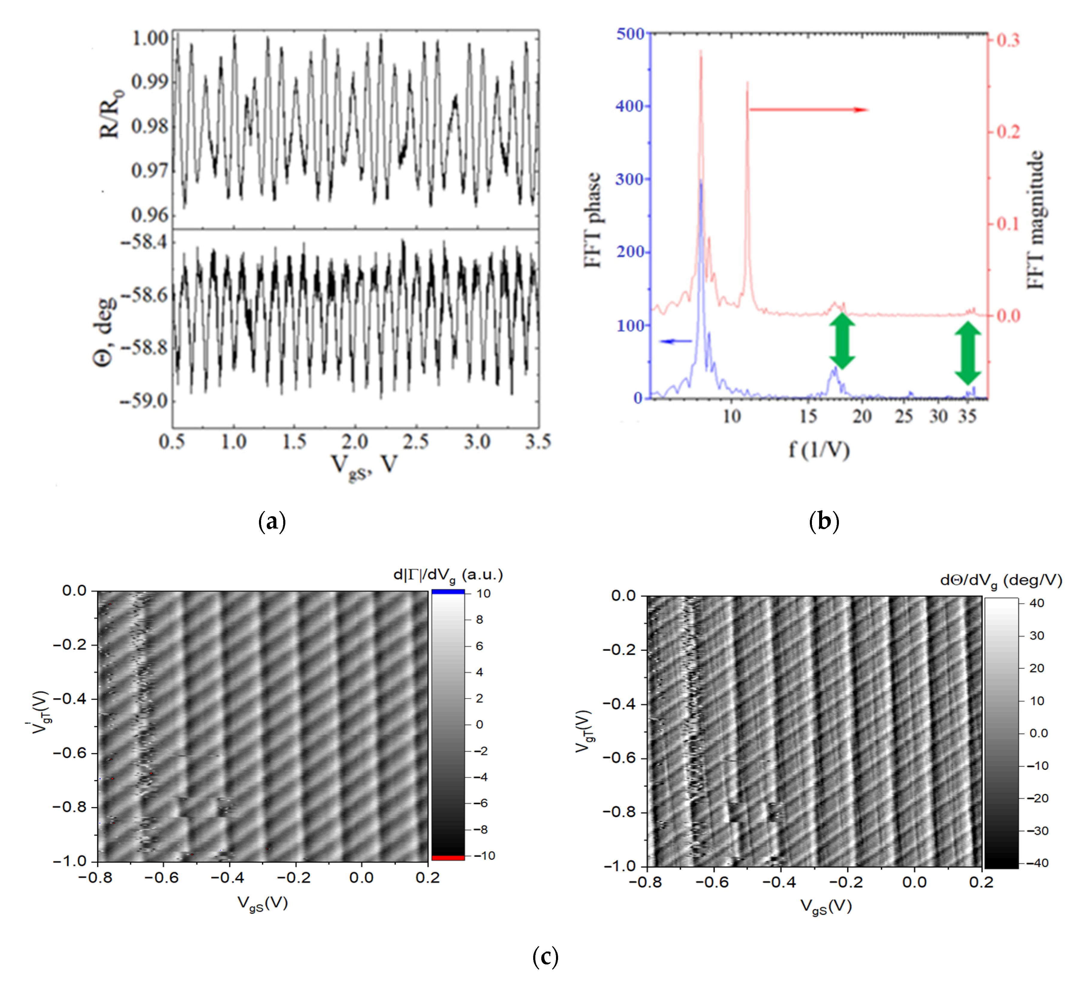
5.2.1. Characterization of a Small (N = 3) SEBA

As shown theoretically in Section 2 and confirmed experimentally in Section 5.1, the SNR for the reflectometry response of a single SEB is low due to very small magnitude of admittance oscillations caused by single electron charging even if an optimized MN described in Section 3 is used. Recently, we have demonstrated that for small SEBA SNR scaling by a factor N is achievable [33]. To study the sensitivity trends in SEBA with resolvable individual characteristics, we performed a detailed study of a small array nominally composed of four SEBs and controlled by two gates in the range of temperatures from 0.3 to 30 K. Post-experimental SEM image of the array is presented in Figure 10a. Figure 10b shows the equivalent circuit of MN used in an experiment tuned close to a matching point by a capacitor CIN = 28.2 pF, and Figure 10c presents the results of MN characterization vs. carrier frequency at T = 11.5 K, which shows a nearly perfect match.
The results of the SEBA response measurements at temperature 11.5 K are presented in Figure 11a as the two respective magnitude d|Γ|/dVg and phase dΘ/dVg, derivatives (solid lines in two subplots). The beating pattern, expected for the addition of asynchronous periodic signals with similar periods is clearly visible. The FFT spectrum of the beating pattern of oscillations acquired over the 16 V Vg span (Figure 11b) unveiled the presence of three primary “frequencies” in 1/V units (A1, B1 and C1) corresponding to the three distinct periods of Coulomb blockade oscillations (respective gate capacitances): A1: 1/53.3 mV (3.0 aF), B1: 1/57.2 mV (2.8 aF) and C1: 1/56.7 mV (2.7 aF). Indeed, post-experimental inspection of this array under SEM revealed a fabrication defect for one SEB (delineated by a dashed white line in Figure 10a) reducing the number of functional devices to three. The FFT spectrum also indicates that at T = 11.5 K signals generated by SEBs are almost sinusoidal, i.e., with clear dominance of the 1st harmonic. The magnitudes of the 2nd harmonics are hardly visible and signals from higher harmonics fell below the noise floor. Superimposed with experimental data are oscillations of d|Γ|/dVg and phase dΘ/dVg (red in Figure 11a) simulated for 3 SEB using Formula (2), which are then passed through the MN depicted in Figure 10b. For simulations, the values of the three gate capacitances are extracted from the FFT plot acquired over the 16 V Vg span. The values of junction capacitances 32, 34 and 28 aF and respective junction resistances, 80, 70 and 100 kΩ for the three respective SEBs are obtained by generating oscillations of SEBA admittance using (2), passing it through the MN shown in Figure 10b and then fitting the magnitude of oscillations in the reflected signal to the experimental data. The initial value of junction resistance is evaluated based upon junction resistance of SETs fabricated in a close proximity to SEBA with the same geometry of island and junction (see Figure 1a,b). The close match of relative amplitudes in FFT (Figure 11b) confirmed a reasonable choice of junction parameters. It is worth noting that at this relatively high temperature, the dominant contribution in formula (2) came from the second term (“Cbox”) related to dynamic capacitance since tunneling rates (fT = γ/2π ≈ 20 GHz at 11.5 K for a 100 kΩ tunneling resistor (2)) are much higher than the RF excitation frequency (461 MHz). To investigate temperature limits for the use of SEB arrays we studied how oscillations of reflected signal wash away with increasing temperature, Figure 11c. It can be seen from this plot that oscillations became hardly distinguishable from the background noise at highest T ≈ 25 K. The device with the smallest total capacitance is expected to exhibit oscillations until temperature fluctuations overcame the charging energy EC~kBT. The estimation of charging energy based upon the comparison experiment and simulations in Figure 11a yields CJ + Cg = 31 aF neglecting all other capacitors. This gives the value for charging energy ECe2/2(Cg + CJ) = kB 30 K or 2.58 meV, in good correlation with the experiment.
Voltage gain for an SET is determined by the ratio α set = C g / C j , so that enhanced coupling to the gate increased the gain. Likewise, this ratio determined the voltage sensitivity of an SEB. To obtain higher sensitivity, it is best to design the sensing gate to maximize this ratio within the available capacitance budget (α > 0.1). For array applications, the operating point needs to be chosen on the steepest slope of constructive interference peaks. If each SEB in the array is coupled to the sensing gate using nominally the same C (i)S = CS, it might be difficult to choose the operating point at a specific gate bias Vg_sens due to random charge offset. For instance, it is difficult to obtain high sensitivity if sensing needs to occur near Vg = 1.05 V in Figure 11a, because of the destructive interference. To enable flexibility of choice for the operating point, a second, tuning gate, with capacitance C(i)t that couples the i-th SEB in the array can be added (see Figure 9a). These capacitors (i.e., C(i)t) can be designed to be intentionally dissimilar (e.g., linearly decreasing) to ensure the placement of the operating point to the steepest slopes of constructive interference peaks within the reachable span of the tuning gate voltage, Vg tune. To illustrate this technique, an example of the reflectometry signal obtained from the same array, now coupled to two gates is presented in Figure 12. In Figure 12a, in the top and bottom subplots sharp lines represent respective derivatives that define sensitivity in magnitude and phase with respect to changing gate bias, d|Γ|/dVg (upper left plot) and dΘ/dVg (bottom left plot) of the reflected signal. Each SEB generates a set of lines with a distinct slope V g t u n e / V g s e n s = C g s e n s / C g t u n e . Constructive interference peaks appear at the points of line crossings. Note that the spacing between lines in each SEB along the V g s e n s axis is almost the same, while along the V g t u n e axis it is distinctly different, indicating dissimilar capacitance C g t u n e for each SEB. To achieve weak and dissimilar coupling tuning gate can be simply positioned on the side of the array [33]. This combination ensures the appearance of line crossings within an easily accessible span of V g t u n e . Near these line crossings, one can find the points of maximum sensitivity where derivatives reach their extrema clearly visible at “knots” on the plot (there are eight such “knots” in Figure 12a). Clearly, the use of a second gate makes it easier to reach a high-sensitivity crossing point where the signals add up (and extrema of respective derivatives can be chosen as “sweet spots” for the sensing application) within a given Vg span, since to find such a point with a single gate would require a much broader span of V g s e n s . This example illustrates that the presence of the secondary gate greatly reduced the necessary V g s e n s span in the search for a constructive interference peak as a point of highest sensitivity.
Note, however, that in the case of very large ratios of EC/kBT ≥ 100 signals generated by each SEB start looking like periodic “delta-functions like” (Figure 8) with a very narrow voltage span for each peak leading to a collapse of overlapped regions and a disappearance of constructive interference peaks.
Curiously, in the dΘ/dVg signal (lower panels in Figure 12) one of the lines, with the steepest slope, had a significantly stronger appearance compared to the other two while in d|Γ|/dVg plots the strength of the signal from each SEB are almost equal. We performed simulations of the response for this array using parameters of SEBs obtained from higher temperature measurements in Figure 11. However, to obtain a good fit to the experimental data in the simulated dΘ/dVg response, the resistance of the two junctions, corresponding to the two lines with poor contrast in this plot need to be increased by almost an order of magnitude. The reason for that likely stems from incomplete suppression of superconductivity in the two SEBs in the array at T < 0.5 K. Opening of the gap in the density of states at the metal-superconductor transition drastically reduces the tunneling rate at zero bias due to a lack of available quasiparticles. This is confirmed by the disappearance of the reflected signal from the SEB if no magnetic field is applied for temperatures T < TC ≈ 1.05 K, where TC is critical temperature for Al. Indeed, in our experimental setup with small permanent magnets the superconducting gap is not completely suppressed in about 50% of the samples. Due to tunnel rate reduction in the two SEB with developing the superconducting gap, the admittance there started to be dominated by Sisyphus resistance while significant reduction in dynamic capacitance term in (2), in turn, resulted in the greatly reduced phase swings at the charge degeneracy points.

5.2.2. Comparative Characterization of Larger (“N = 40” vs. “N = 200”) SEBAs

As discussed in Section 2, utilization of N SEBs in an array is expected to enhance the “collective” oscillation magnitude by a factor of ~ N . While accurate quantitative comparison between experimentally obtained and simulated response of arrays can only be performed for a properly calibrated (i.e., error-corrected) system, an accurate qualitative comparison between arrays of a different size, N, can be performed for arrays of a different size simultaneously connected to the same MN. In this setup, each array is biased with its own gate like it is shown in Figure 4c (for simplicity each array is represented as a single SEB). To reduce cross-coupling the values of capacitances C21 and C12 need to be much smaller than sensing gate capacitances C11 and C22 in Figure 4c. In the experiment, this is achieved by picking two arrays separated by about 5 mm on a chip. A block-diagram of the experiment where two important parameters characterizing sensitivity, d|Γ|/dVg and dΘ/dVg are acquired simultaneously for two arrays with a nominal size N = 40 and N = 200 SEB is presented in Figure 13. Note that since the SEB is a two-terminal device, its admittance can be probed either way (see Section 5.2.3 for further discussion); in this experiment both arrays had their sensing gates tied together. In addition to the ramp voltage, Vg, small modulation signals with a magnitude of 0.5 mV and frequency of f1 = 1.45 kHz and f2 = 2.48 kHz are applied to the common sources of 40 SEB and 200 SEB arrays, respectively. The reflectometry setup utilized the MN tuned at 305.7 MHz and homodyne reflectometer (labeled “R” in Figure 12a, see Figure 4a for details) followed by two synchronous demodulators operating at frequencies f1 and f2. For this purpose, the bandwidth of ZI UHF demodulator is set to pass the signals at frequencies f1 and f2 without attenuation. The signals d|Γ|/dVg and dΘ/dVg are obtained for both 40 SEB and 200 SEB arrays by performing a second demodulation using two low-frequency lock-ins operating at f1 and f2. The results of the experiment are presented in Figure 13b where d|Γ|/dVg and dΘ/dVg are shown for both the 40 SEB array (blue) and 200 SEB array (red). Curve averaging (58 ramps, about 25 s each) is used to boost SNR by a factor ≈7.6; the equivalent BW of the signals presented in Figure 13b is 26 Hz. The results, however, indicate that the ratios of magnitudes of peaks in both derivative signals deviate from the expected value of (200/40)1/2 ≈ 2.23 as the 200SEB array signal appeared to be >4 times stronger than that from the 40 SEB array. The likely cause for this discrepancy is the presence of fabrication defects, which might result in a reduction of the number of functional devices. An SEM micrograph Figure 13c shows several examples of such defects (observed in a different device). It is clear that only half of the inspected devices on that sample, namely the SEBs above the gate line, are functional. Simulations indicate that the observed ratio of 4 in signal strength suggests that the actual ratio of functional devices in the 200 SEB vs. 40 SEB array is close to 16, rather than 5.

5.2.3. Experimental Characterization of SEB Arrays with Different Matching Networks

In Section 3.2 above, we discussed design choices for building a matching Π network suitable for SEB applications. Figure 6 indicates that a significant boost of sensitivity can be achieved with a simple adjustment of a single capacitor CIN. To verify this, we perform an experiment to compare the response from the same array of 200 SEBs for different values of input capacitance CIN, Figure 14. In this example, the MN is composed of L = 270 nH inductor, pad capacitor Cpad~0.55 pF and two selected values of CIN. The results of measurements for the two derivatives, dR/dVg and /dVg at two different values of this capacitor are presented in Figure 14a,b. The results show more than 10 times enhancement of the (phase-gate voltage) sensitivity factor, dΘ/dVg. Note that the enhancement of the magnitude response is less pronounced, leading to about a 5-fold boost in the signal in good agreement with simulations in Figure 6. It is also worth noting that according to the simulations the accessible bandwidth is narrower for the network settings close to a match point CIN = 27 pF (≈2.2 MHz) compared to the overcoupled case CIN = 18 pF (≈3.3 MHz).
Figure 15 shows a 2D map of derivative dRe(Γ)/dVg versus two gate voltages, Vg sens and Vg tune, with an apparent moire pattern resulting from multiple line crossings. In comparison with Figure 12, discrimination between individual lines representing individual SEBs is no longer possible. Moreover, multiple line crossings in Figure 15a produced “bunching”—an effect that appears to look like a sharp line over a smaller 2D region but visibly fades away on a larger scale—an effect typical for moire patterns. Indeed, crossing lines create that appears as oscillations with a period much shorter than that of a single SEB despite the same gate coupling for each individual box.
Most importantly, as discussed for the case of 3 SEBs (Figure 12), the use of a second gate provides means for finding the most sensitive spots for any desired sensing gate region. These most sensitive spots corresponding to extrema in the derivative are delineated by a color change (from red = max, to blue = min) in Figure 15. A plot for the simulated response for 200 SEB array is shown in Figure 15b where it is clearly similar to the experiment.

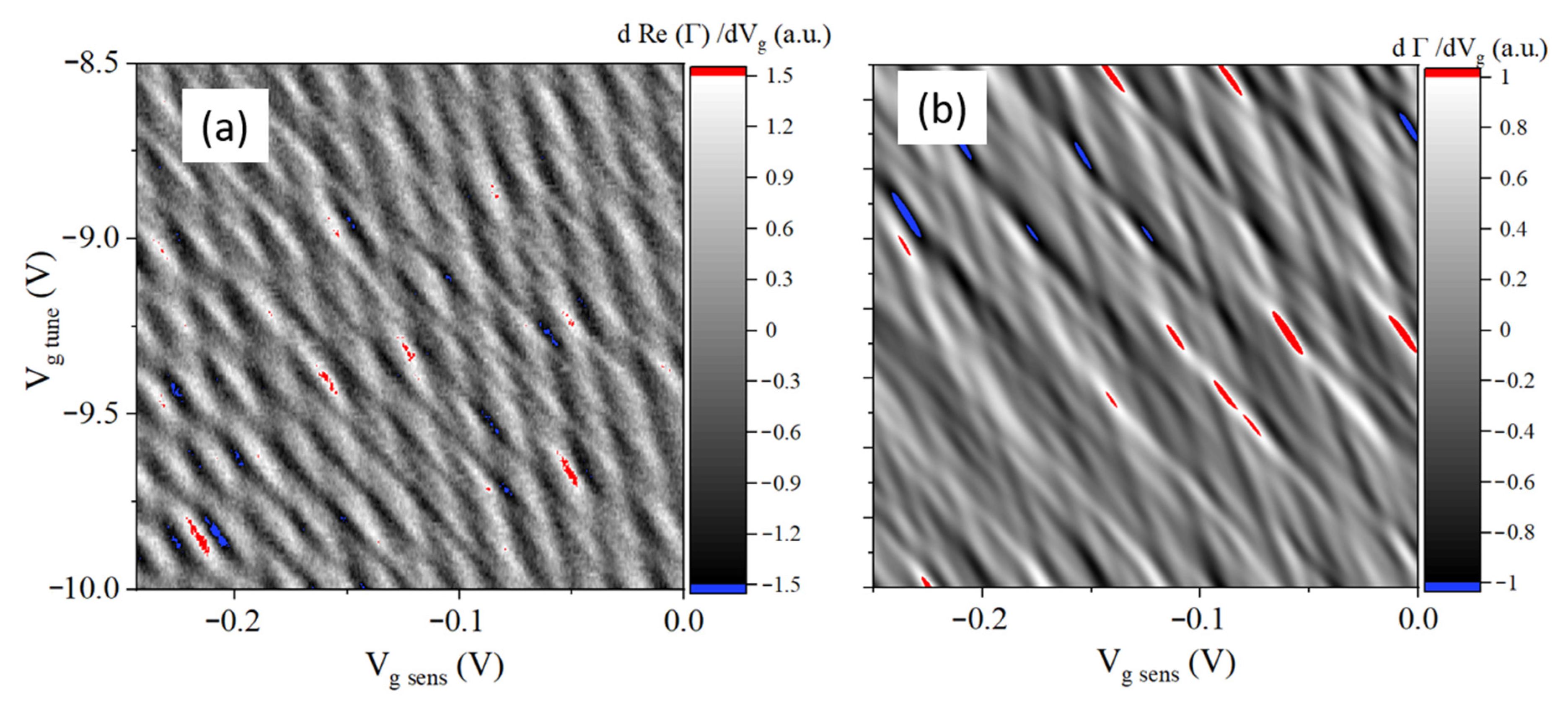
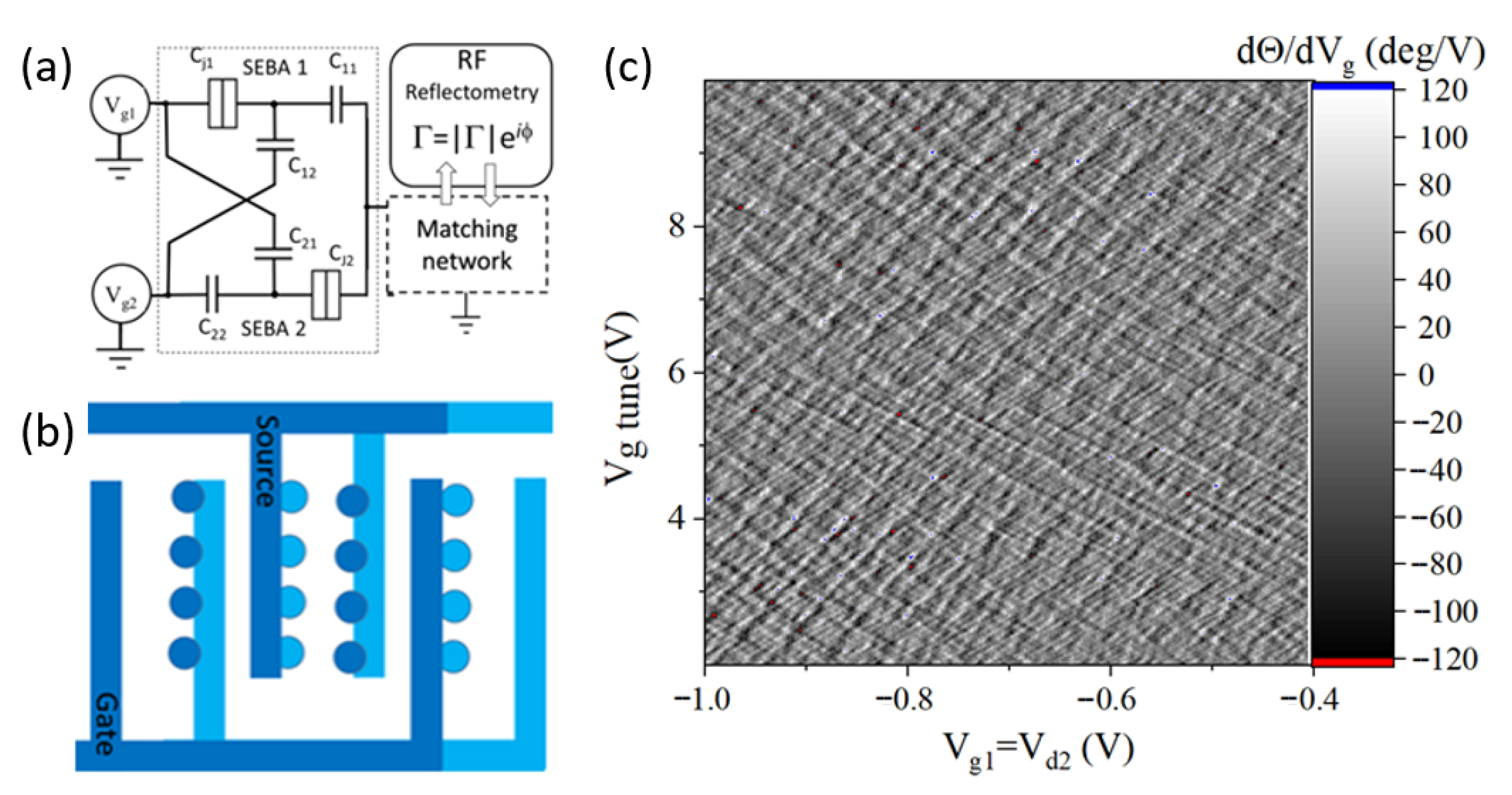
5.2.4. Characterization of Cross-Coupled SEB Arrays

Note that the slopes of crossing lines in Figure 12 and Figure 15 are always negative because with SEB junctions at ground potential any combination of capacitive gates had an additive effect, i.e., in the presence of positive (negative) voltage at one gate it took a lesser (larger) value of positive (negative) voltage on the other gate to reach the charge changing state: Qg = C1V1 + C2V2. The “counter-parallel” connection of devices shown schematically in Figure 16a ensures that charging processes in array SEBA 1 and SEBA 2 (for simplicity represented as one junction) go in the opposite directions. For instance, by increasing positive voltage Vg1 electrons are added to SEBA 1 and at the same time removed from SEBA 2. This configuration is therefore expected to yield lines with both positive and negative slopes thus greatly increasing the number of interfering points. A way to design such a device using Dolan bridge technique with a small footprint and a large density of SEBs is to use the interdigitated design with alternating placement of SEB islands, as schematically shown in Figure 16b. One of the electrodes labeled “source” is connected to a MN while the other labeled “gate” is used as a sensing gate. The tuning gate would be located farther away from the structure and it needs to have much weaker coupling to the SEBA. In the experiment we use two separate SEBA with nominal N = 200 in each and simply connect them as shown in Figure 16a. The expected line crossing pattern is observed in the experiment, Figure 16c, where multiple outstanding extrema are occurring all over the map.

5.3. Comparison of Performance between SEB Array and DC-Decoupled SET

For practical applications we need to make sure that the advantages of the N-sized SEB array approach, such as doubling of operating temperature and a smaller footprint per device are worth pursuing compared to more conventional approaches that utilize an RF SET as a sensing element. Here, we exploited a variation of the RF SET, which we call a “DC decoupled-SET” (DCD SET), Figure 17a. The key feature of this design is the lack of DC path through the SET device: either one or both junctions are connected to the outside only through a coupling capacitors ~0.5 pF between bonding pads defined by optical lithography. This resulting device is protected against accidental ESD due to the lack of a DC path. The impedance of the 0.5 pF capacitor at high frequencies (2 kΩ at 160 MHz) became negligible compared to RSET > 50 kΩ, so it has little effect on the measured impedance at these frequencies. To compare performance of DCD SET with a SEBA, we set up an experiment a circuit diagram for which is shown in Figure 17b and a physical layout is represented by a micrograph Figure 17c. The performance of the array composed of four SEBs is directly compared with that of two SETs AC drain-coupled to the same resonator. In an SEB the capacitance between the gate and the SEB island is a part of the total “island to outside world” capacitance, and thus while larger gate capacitance has the benefits of enhancing the total admittance of the device Y(Vg), it also leads to a reduction of charging energy. By contrast, in the DCD SET the maximal admittance is set primarily by the resistance of the tunnel junctions and is independent of the gate capacitance. Note that for the structure shown in Figure 17c the gate capacitance for the SETs is approximately 2 times smaller than that of SEB due to different gate proximity.
The results of the RF reflectometry measurements of a combined structure composed of four SEBs and two DCD SETs are presented in Figure 18. The distinct beating pattern is clearly visible in Figure 18a (upper panel, magnitude plot). FFT analysis of the spectral composition of this signal shows that it is predominantly composed of two prime components (8.5 V−1 and 10.5 V−1, red curve in Figure 18b) and several higher frequency components of much smaller magnitude bunching around 18 V−1 and 36 V−1. These higher frequency components are also present in the FFT of phase (blue curve in Figure 18b), while one of the lower frequency components (10.5 V−1) became practically undetectable.
To identify the origin of the observed signals a 2D maps of the derivatives d|Γ|/dVg and dΘ/dVg in coordinates VgS and VgT are obtained (Figure 18c). The pattern on the left panel shows the appearance of two distinct sets of lines: the one with a positive slope and another one with a negative slope, corresponding to a 10.5 V−1 and 8.5 V−1 spectral component in the FFT in Figure 18b. This set of lines is exactly what is expected from the counter-parallel connection of SETs. The signal stemming from a “fully-floating” DCD device yields a different phase compared to the SET DC-drain coupled to VgT in Figure 17c. On closer inspection a series of faint lines are also visible in the phase plot of Figure 18c. One can also speculate that these lines correspond to signatures of SEBs visible in FFT of Figure 18b with inverse periods of 16–18 V−1 (first harmonic) and 32–26 V−1 (second harmonic), since the physical layout for SEBs in this experiment is exactly the same as in for the device with three SEBs discussed above (Figure 10, Figure 11 and Figure 12). However, the closeness of the second harmonic of the signal 2 × 8.5 = 17 V−1 generated by the DCD SET makes it impossible to accurately identify the SEB signature in FFT.
To further investigate SEBs and perform an accurate comparison, in the next experiment both DCD SETs are “muted” by shorting their source and drain electrodes thus making both of SETs grounded for AC. This converts the measured sample into just an array of 4 SEBs. The experiment is then repeated, and comparative performance of the two configurations (two SETs plus four SEBs) vs. four SEBs is presented in Figure 19a,b where the respective derivatives are plotted for the two cases. 2D map of phase derivative oscillations dΘ/dVg is shown in Figure 19c where only lines of negative slopes are observed as expected for SEBA with DC grounded sources, and a typical oscillation “frequency” of about 20 V−1. It is clear that the four SEBs device yields much weaker (by more than an order of magnitude) signal in magnitude of reflection but exhibited noticeable signal strength in phase of the reflected signal. Taking into account sensitivity scaling ~ N1/2 a nine times larger SEBA (N ≥ 4 × 9) is needed to reach the phase sensitivity, and N ≥ 4 × 400 SEBA is needed to reach the magnitude sensitivity of a single DCD SET. (Here we also took into consideration the doubling of the sensitivity in the maxima for the two SETs, counterbalanced by approximately two times smaller Cg coupling to the SETs). This confirms the trends discussed in Section 2 (Figure 3e).

6. Conclusions

The results of the experiments show that the concept of using arrays of SEB for sensing applications is comparable to other devices, such as SETs, and it brings several important advantages, such as elevated operating temperatures, a smaller device footprint and inherent protection from ESD damage. We experimentally confirmed the results of simulations for estimating the number of SEBs needed to outperform drain-coupled RF SET. With the SEB design used throughout the experiments (Cg sense ~ 3 aF) this number is fairly large, N > 1000. Our simulations show, however, that within the same “capacitive budget” as in the studied SETs, a 100 times improvement in performance for SEBs could be obtained simply by enhancing the sensing gate capacitance. The practicality of an array of SEBs is greatly improved by including a second tuning gate to find a maximum sensitivity point over a smaller voltage range. A considerable improvement in the sensitivity of an optimally designed MN is also demonstrated. The advancements we developed in the area of SEB applications created greater potential to use these sensors in a wider array of applications. The experimentally observed relative ESD immunity compared to traditional SETs stems from two factors: a) lack of DC path through the device, which prevents device destruction upon application of large biases (up to 40 V tested) and b) capacitive voltage division in series CgCJ chain, which for the case of CJ >> Cg leads to significant (>10) attenuation of any spurious voltage across CJ and thus prevents its destruction. A conceptually similar device, a “DC-decoupled SET” appears to provide a reasonable compromise between SEB and traditional SET and has to be further explored for use as more rugged sensors in applications where the devices cannot be protected from exposure to large potentials. Increasing the charging energy through further reduction in the total capacitance may also yield devices that can provide the highly sensitive electrometers at elevated temperatures, potentially up to the range accessible by liquid nitrogen (77 K).

Supplementary Materials

The following are available online at https://www.mdpi.com/2076-3417/10/24/8797/s1. Figure S1: Printed circuit board with two RF ports.

Author Contributions

T.A.Z. designed and fabricated all of the devices and participated in measurements; M.J.F. participated in measurements, designed and implemented software analysis tools for MNs and SEB simulations; J.C. supervised MN design and signal analysis; M.H. participated in MN experiments and performed analysis of MNs; E.D.-F. and J.R. participated in ultra-low temperature measurements; A.O.O. designed and ran experiments and performed data analysis and simulations; G.L.S. participated in design of experiments and data analysis; X.J. and M.S. designed the RF test boards and assisted in the design and implementation of experiments. The manuscript was written by T.A.Z., A.O.O., and M.J.F. and edited by all authors. All authors have read and agreed to the published version of the manuscript.

Funding

This research was funded by the US National Science Foundation grants DMR-1904610 and ECCS-1509087.

Acknowledgments

The author are thankful to Anwesha Palit for reading the manuscript and making multiple suggestions.

Conflicts of Interest

The authors declare no conflict of interest.

References

  1. Likharev, K.K. Single-electron devices and their applications. Proc. IEEE 1999, 87, 606–632. [Google Scholar] [CrossRef] [Green Version]
  2. Brenning, H.; Kafanov, S.; Duty, T.; Kubatkin, S.; Delsing, P. An ultrasensitive radio-frequency single-electron transistor working up to 4.2 K. J. Appl. Phys. 2006, 100, 114321. [Google Scholar] [CrossRef] [Green Version]
  3. Su, L.; Xinxing, L.; Hua, Q.; Xiaofeng, G. A sensitive charge scanning probe based on silicon single electron transistor. J. Semicond. 2016, 37, 044008. [Google Scholar] [CrossRef]
  4. Suter, K.; Akiyama, T.; De Rooij, N.F.; Huefner, M.; Ihn, T.; Staufer, U. Integration of a Fabrication Process for an Aluminum Single-Electron Transistor and a Scanning Force Probe for Tuning-Fork-Based Probe Microscopy. J. Microelectromechanical Syst. 2010, 19, 1088–1097. [Google Scholar] [CrossRef]
  5. Yoo, M.J.; Fulton, T.A.; Hess, H.F.; Willett, R.L.; Dunkleberger, L.N.; Chichester, R.J.; West, K.W. Scanning single-electron transistor microscopy: Imaging individual charges. Science 1997, 276, 579–582. [Google Scholar] [CrossRef] [PubMed]
  6. Brenning, H.T.; Kubatkin, S.E.; Erts, D.; Kafanov, S.G.; Bauch, T.; Delsing, P. A single electron transistor on an atomic force microscope probe. Nano Lett. 2006, 6, 937–941. [Google Scholar] [CrossRef]
  7. Aassime, A.; Johansson, G.; Wendin, G.; Schoelkopf, R.J.; Delsing, P. Radio-frequency single-electron transistor as readout device for qubits: Charge sensitivity and backaction. Phys. Rev. Lett. 2001, 86, 3376–3379. [Google Scholar] [CrossRef] [Green Version]
  8. Bladh, K.; Gunnarsson, D.; Johansson, G.; Käck, A.; Wendin, G.; Aassime, A.; Delsing, P. Reading out charge qubits with a radio-frequency single-electron-transistor. In Condensation and Coherence in Condensed Matter. Proceedings of the Nobel Jubilee Symposium, Goteborg, Sweden, 4–7 December 2001; The Royal Swedish Academy of Sciences: Stockholm, Sweden, 2002. [Google Scholar]
  9. Crippa, A.; Maurand, R.; Bourdet, L.; Kotekar-Patil, D.; Amisse, A.; Jehl, X.; Barraud, S. Electrical Spin Driving by $g$-Matrix Modulation in Spin-Orbit Qubits. Phys. Rev. Lett. 2018, 120, 137702. [Google Scholar] [CrossRef] [Green Version]
  10. Gonzalez-Zalba, M.F.; Barraud, S.; Ferguson, A.J.; Betz, A.C. Probing the limits of gate-based charge sensing. Nat. Commun. 2015, 6, 1–8. [Google Scholar] [CrossRef] [Green Version]
  11. Hollenberg LC, L.; Wellard, C.J.; Pakes, C.I.; Fowler, A.G. Single-spin readout for buried dopant semiconductor qubits. Phys. Rev. B 2004, 69, 233301. [Google Scholar] [CrossRef] [Green Version]
  12. Kotekar-Patil, D.; Corna, A.; Maurand, R.; Crippa, A.; Orlov, A.; Barraud, S.; Sanquer, M. Pauli spin blockade in CMOS double quantum dot devices. Phys. Status Solidi B 2017, 254, 1600581. [Google Scholar] [CrossRef]
  13. Morello, A.; Escott, C.C.; Huebl, H.; Van Beveren, L.W.; Hollenberg LC, L.; Jamieson, D.N.; Clark, R.G. Architecture for high-sensitivity single-shot readout and control of the electron spin of individual donors in silicon. Phys. Rev. B 2009, 80, 081307. [Google Scholar] [CrossRef] [Green Version]
  14. Petersson, K.D.; Smith, C.G.; Anderson, D.; Atkinson, P.; Jones GA, C.; Ritchie, D.A. Charge and spin state readout of a double quantum dot coupled to a resonator. Nano Lett. 2010, 10, 2789–2793. [Google Scholar] [CrossRef] [PubMed] [Green Version]
  15. Niemeyer, J. Eine einfache Methode zur Herstellung kleinster Josephson-Elemente. Ptb Mitt. 1974, 84, 251–253. [Google Scholar]
  16. Dolan, G.J. Offset works for lift-off photoprocessing. Appl. Phys. Lett. 1977, 31, 337–339. [Google Scholar] [CrossRef]
  17. Lafarge, P.; Pothier, H.; Williams, E.R.; Esteve, D.; Urbina, C.; Devoret, M.H. Direct observation of macroscopic charge quantization. Z. Phys. B 1991, 85, 327–332. [Google Scholar] [CrossRef]
  18. Schoelkopf, R.J.; Wahlgren, P.; Kozhevnikov, A.A.; Delsing, P.; Prober, D.E. The radio-frequency single-electron transistor (RF-SET): A fast and ultrasensitive electrometer. Science 1998, 280, 1238–1242. [Google Scholar] [CrossRef] [Green Version]
  19. Zimmerli, G.; Kautz, R.L.; Martinis, J.M. Voltage gain in the single-electron transistor. Appl. Phys. Lett. 1992, 61, 2616–2618. [Google Scholar] [CrossRef]
  20. Kafanov, S.; Delsing, P. Measurement of the shot noise in a single-electron transistor. Phys. Rev. B 2009, 80, 155320. [Google Scholar] [CrossRef] [Green Version]
  21. Gustavsson, S.; Gunnarsson, D.; Delsing, P. Cryogenic amplifier for intermediate source impedance with gigahertz bandwidth. Appl. Phys. Lett. 2006, 88, 153505. [Google Scholar] [CrossRef]
  22. Persson, F.; Wilson, C.M.; Sandberg, M.; Johansson, G.; Delsing, P. Excess Dissipation in a Single-Electron Box: The Sisyphus Resistance. Nano Lett. 2010, 10, 953–957. [Google Scholar] [CrossRef] [PubMed] [Green Version]
  23. Luryi, S. Quantum capacitance devices. Appl. Phys. Lett. 1988, 52, 501–503. [Google Scholar] [CrossRef]
  24. Mizuta, R.; Otxoa, R.M.; Betz, A.C.; Gonzalez-Zalba, M.F. Quantum and tunneling capacitance in charge and spin qubits. Phys. Rev. B 2017, 95, 045414. [Google Scholar] [CrossRef] [Green Version]
  25. Zimmerman, N.M.; Keller, M.W. Dynamic input capacitance of single-electron transistors and the effect on charge-sensitive electrometers. J. Appl. Phys. 2000, 87, 8570–8574. [Google Scholar] [CrossRef]
  26. Frake, J.C.; Kano, S.; Ciccarelli, C.; Griffiths, J.; Sakamoto, M.; Teranishi, T.; Buitelaar, M.R. Radio-frequency capacitance spectroscopy of metallic nanoparticles. Sci. Rep. 2015, 5, 10858. [Google Scholar] [CrossRef] [PubMed] [Green Version]
  27. Beenakker, C.W.J. Theory of Coulomb-blockade oscillations in the conductance of a quantum dot. Phys. Rev. B 1991, 44, 1646–1656. [Google Scholar] [CrossRef] [PubMed] [Green Version]
  28. Filmer, M. Development of High Speed Nanoscale Sensors Based on Single-Electron Devices. Ph.D. Thesis, Univeristy of Notre Dame, Notre Dame, IN, USA, 2020. [Google Scholar]
  29. Chisum, J.D.; Popovic, Z. Performance limitations and measurement analysis of a near-field microwave microscope for nondestructive and subsurface detection. IEEE Trans. Microw. Theory Tech. 2012, 60, 2605–2615. [Google Scholar] [CrossRef]
  30. Bray, J.R.; Roy, L. Measuring the unloaded, loaded, and external quality factors of one- and two-port resonators using scattering-parameter magnitudes at fractional power levels. IEEE Proc. Microw. Antennas Propag. 2004, 151, 345–350. [Google Scholar] [CrossRef]
  31. Ares, N.; Schupp, F.J.; Mavalankar, A.; Rogers, G.; Griffiths, J.; Jones, G.A.C.; Briggs, G.A.D. Sensitive Radio-Frequency Measurements of a Quantum Dot by Tuning to Perfect Impedance Matching. Phys. Rev. Appl. 2016, 5, 034011. [Google Scholar] [CrossRef]
  32. Zirkle, T.A. A parallel single-electron box array scanning probe. In Electrical Engineering; University of Notre Dame: Notre Dame, IN, USA, 2019; p. 189. [Google Scholar]
  33. Filmer, M.J.; Zirkle, T.A.; Chisum, J.; Orlov, A.O.; Snider, G.L. Using single-electron box arrays for voltage sensing applications. Appl. Phys. Lett. 2020, 116, 213103. [Google Scholar] [CrossRef]
Figure 1. Schematic diagrams and scanning electron micrographs of a single electron transistor (a) and single electron box (b) fabricated by the Dolan bridge technique. The scale bar is the same for both cases. (c) Simplified circuit diagram of the experiment in [17] where the single-electron transistor (SET), delineated by a red dashed line, is employed to probe single-electron charging in single-electron box (SEB), delineated by a blue dashed line. The SEB is coupled to the SET using a coupling capacitor CC. (d) Functional diagram of the SEB measurement by an RF reflectometry setup. RSis and Cdyn represent contribution to the change in total impedance of SEB from Sisyphus resistance and dynamic capacitance. These two effects associated with single electron tunneling in and out of SEB cause variations in the matching network and thus affect the reflected signal.
Applsci 10 08797 g001
Figure 2. Complex admittance oscillations vs. Vg and respective components of it (a) magnitude; (b) phase; (c) inverse of Sisyphus resistance and (d) dynamic capacitance for single SEB calculated using Formula (1) at two temperatures: 50 mK (blue) and 4.2 K (red).
Applsci 10 08797 g002
Figure 3. (a) Single SEB circuit symbol. (b) Frake model of an SEB as parallel frequency dependent conductance and capacitance. (c) Circuit schematic of the SEB array. (d,e) Simulated trends of signal strength (derivatives) d|Y|/dVg and dΦ/dVg as a function of the number of SEB in the arrays at 2.4 K with junction parameters listed in the text. (d) Normalized signal strength of the two derivatives: magnitude (black) and phase (red) of admittance for SEBA of varying size. Each data point is the average of 100 simulations of the same array conditions with randomization to account for process variation. (e) Simulations for magnitude sensitivity for SEBA with different average gate capacitances: Cg = 22.9 aF (green), and Cg = 2.9 aF (black). The solid (dashed) black and solid (dashed) green lines correspond to a Vg search range of 10 V (100 mV). The blue dashed line corresponds to the response from a single SET with indicated capacitances and RS = RD = RJ = 50 kΩ biased at the maximum sensitivity point.
Applsci 10 08797 g003
Figure 4. (a) Simplified circuit diagram of the single-port reflectometry setup. Circuit delineated by a dashed line is the sample attached to the PCB board with the MN and cooled to a temperature defined by the setup; the MN circuitry is outlined in a red box with port 1 facing the sample and port 2 facing the directional coupler. Blue rectangle delineates the cryogenic part of the measurement apparatus. Amplifier at 40 K, ZX60-P33ULN+ is thermally anchored to the 1st stage of the cryocooler, T ≈ 40 K; two stage amplifier at room temperature uses ZX60-P103LN+; both types of amplifiers are by Mini-Circuits. Directional coupler ZFDC-20-50-S+ and cold attenuator are located at the second stage of cryocooler @2.7 K (Janis He3, Bluefors) or 3.5 K (ARS). The PCB with the sample is bolted to the He3 pot (Janis He3); mixing chamber sample exchange platform (Bluefors) or 2nd stage of cryocooler (ARS). (b) Block diagram of the experiment with a SEB array coupled to two gates with capacitances C11C1n to Vg1 (“sensing gate”) and C21C2n to Vg2 (“tuning gate”). (c) Block diagram of the experiment for comparative measurements of two arrays. The junction sides of the SEBs for both arrays are connected to the same MN. For simplicity each array is shown as a single SEB. The devices are spatially separated on the chip to minimize capacitive crosstalk.
Applsci 10 08797 g004
Figure 5. Temperature dependence of the DC resistance of the 390 nH Coilcraft 0805 inductor (red) and 43 pF Johansson technology capacitor (black).
Applsci 10 08797 g005
Figure 6. (a) Circuit diagram of a Π-MN used in measurements. CIN is a tuning element; CPAD is a bond pad capacitor; horizontally places elements between CIn and CPAD represent the realistic inductor at low temperature; a single SEB with parameters similar to the experiment is attached to a bond pad. (b) Magnitude and phase response of the MN for three different values of CIN indicated in the plot: blue, 20 pF; green, 28.2 pF; and red, 40 pF. Inset table represents −3 dB small signal gate modulation bandwidth calculated in ADS software. (c) Simulated response of the network with an SEB with parameters shown in subplot (a) at T = 2.4 K: Oscillations in magnitude (c1) and phase (c2) of SEB admittance vs. gate bias Vg calculated for carrier frequencies corresponding to the minima in the magnitude of the reflected signal in subplot (b). Derivatives d|Γ|/dVg (c3) and /dVg (c4) of oscillations in the reflected signal.
Applsci 10 08797 g006
Figure 7. (a) MN used for probing single SEB. The values for RDC = 0.02 Ω and RSE = 0.35 Ω at 199 MHz are adjusted for low temperature. The series resistance of parasitic parallel capacitor (57.5 Ω) is tuned to obtain the best fit. The value of parasitic parallel capacitor (260 fF) used in simulations is equal to its room temperature value, while RC (57.5 Ω) is an adjustable parameter. (b) Comparison between the simulated and measured response of the network shown in Figure 7a; upper panel—magnitude and lower panel—phase of reflection. Dashed line—simulations; solid line—experiment.
Applsci 10 08797 g007
Figure 8. Experimentally obtained reflectometry data (blue lines) along with simulations (black lines) for magnitude (a) and phase (b) of the RF signal reflected from SEB. Base temperature of the fridge is 25 mK. Both curves are obtained by averaging of 3049 scans; effective bandwidth is 2.7 kHz. Caclulated oscillations of admittance magnitude (c) and phase (d) using Formula (2) from Section 2. Parameters used in simulations: Cg = 2.88 aF, CJ = 65 aF, RJ = 45 kΩ, T = 50 mK. The calculated phase response is offset by a constant ( −40 degrees) for easy comparison.
Applsci 10 08797 g008
Figure 9. (a) High resolution SEM image of an array composed of 8 SEBs. Probing gate is located in close proximity to the array and has nominally equal coupling to each SEB. Tuning gate is located farther away and is unequally coupled to each SEB element. (b) example of an array composed of a large number of SEBs (> 1000). Small dots below the lines are secondary islands resulting from the Dolan bridge process, and the two horizontal lines leading to the left are the gate. (c) An example of a self-aligned 9 SEB array with a footprint less than 1 × 1 μm2.
Applsci 10 08797 g009
Figure 10. (a) High resolution SEM image of the 3 SEBA (only 3 out of 4 SEBs are operational). The three lines leading to the right are drains that are bonded in parallel to the MN. The vertical line situated about 0.5 μm away from the islands is the probing gate. The tuning gate is situated much farther (about 10 μm) below the entire array (not shown). A fabrication defect for one SEB is delineated by a dashed white line. The data for the 3 SEBA presented below are obtained from this very device. (b) Model of the MN used in simulations. The values of CL = 86 fF and L = 215 nH are from the Coilcraft datasheet. The values of RDC and RSE are both adjusted based on measured resistivity reduction at low temperature; CPAD is calculated by fitting the resonant frequency to the experimental data, and the value of RC is adjusted to obtain the observable depth in the magnitude response. (c) Experimentally obtained (solid lines) and simulated (dashed lines) frequency response of the reflectometry setup using the MN in (b), T = 11.5 K.
Applsci 10 08797 g010
Figure 11. (a) Oscillations of derivatives d|Γ|/dVg and phase dΘ/dVg vs. voltage of sensing gate Vg of the 3 SEB array at 11.5 K superimposed with simulations. Black—experiment, red—simulations. (b) FFT of dΘ/dVg data over 16 V Vg span (black) along with the spectrum of simulated data (red in Figure 11a). (c) Oscillations of the derivative dRe(Γ)/dVg vs. Vg acquired at different temperatures (from 3.9 to 23.5 K).
Applsci 10 08797 g011
Figure 12. (a) Experimentally obtained two dimensional maps of derivatives d|Γ|/dVg (top) and dΘ/dVg (bottom) for the 3 SEB array from Figure 9a. The maps are acquired without curve averaging using an equivalent noise bandwidth of 53 Hz. T = 0.305 K and RF carrier excitation ≈ 50 μV measured at the input of the MN. (b) Simulations of respective derivatives using MN parameters obtained from fitting to the experimentally obtained resonant curve. Junction capacitances for simulations parameters are obtained from Figure 10a: CJi = [32 34 28] aF C(i)S = [2.59, 2.7, 3.16] aF; C(i)t = [0.057 0.129, 0.248] and RJi = [70, 400, 500] kΩ, where i = 1,2,3. The calculation is performed for T = 0.5 K. MN parameters are obtained by a procedure similar to that for Figure 10c, adjusted for lower temperature.
Applsci 10 08797 g012
Figure 13. Comparison of the performance between two SEBA with a nominal number of SEB N = 40 (“40 SEB”, here and below marked blue) and N = 200 (“200 SEB”, here and below marked red) at T = 2.8 K. (a) Simplified block diagram of the experiment with 40 SEB and 200 SEB connected to the same resonator and sharing the same ramp voltage Vg while modulated at two different frequencies, f1 = 1.45 kHz for 40 SEB and f2 = 2.48 kHz for 200 SEB. MN—matching network operating at 305.7 MHz; circles with “+” sign represent adders; R—reflectometer that includes ultra-high frequency lock-in amplifier by Zurich Instruments (ZI UHF) and SR830 lock-ins to extract derivatives by further demodulating the downconverted signals of the ZI lock-in. (b) Comparison of oscillation patterns for derivatives d|Γ|/dVg and dΘ/dVg representing magnitude and phase sensitivity for 40 SEB (blue) and 200 SEB (red) (c) Typical fabrication defects found in the devices inspected under SEM. The number of devices in the micrograph by design is 6, but the entire set of bottom source lines to individual SEB is missing.
Applsci 10 08797 g013
Figure 14. Comparison between the response of the same array of 200 SEB at T = 4.5 K with two different settings of the Π-network (Figure 4a) is composed of L = 270 nH Coilcrtaft 0805CS inductor, Cpad = 0.55 pF and CIN: red—CIN = 27 pF, blue—CIN = 18 pF. (a) Comparison of derivatives d|Γ|/dVg; (b) Comparison of derivatives dΘ/dVg. Comparison of the magnitude (c) and phase (d) characteristics of the two MNs.
Applsci 10 08797 g014
Figure 15. (a) Experimentally acquired two–dimensional map of derivative dRe(Γ)/dVg from a source-coupled 200 SEB array at 0.3 K; (b) simulated response of an array of 200 SEB composed of two 100 SEB subarrays with different coupling to tuning gate. Cg sense = 3 aF with 1% STD (horizontal axis, Vg sens) and Cg tune 1 = 0.2 aF STD 10%, Cg tune 2 = 0.4 aF STD 10% (vertical axis, Vg tune). The contribution of each SEB to the signal is assumed to be equal. The development of the moire pattern is clearly visible. Red (blue) regions correspond to the maxima (minima) of the derivative, where the constructive interference occurs.
Applsci 10 08797 g015
Figure 16. (a) Simplified circuit diagram of the counter-parallel connection of SEB arrays. (b) A sketch of the design featuring the interdigitated design with alternating placement of islands overlapping either source or gate regions. The different shades of blue represent the two evaporation steps of the Dolan bridge technique. The tuning gate is not shown and it can be placed above or below the structure to ensure dissimilar coupling. (c) Experimental 2D map obtained from connecting two nominally identical arrays connected as shown in the circuit diagram. Both arrays nominally contain 200 SEB each.
Applsci 10 08797 g016
Figure 17. (a) Simplified circuit diagram of the DC decoupled-SET (DCD SET). Either one or both junctions are isolated with one or two non-leaky capacitors. (b) Circuit diagram of the experiment: two SETs and four SEBs are connected together to a single MN, with the SETs in counter-parallel configuration, and SEBs in parallel configuration. The lower SET in the diagram is a ”DC-decoupled.” (c) The electron micrograph of the structure used in the experiment. Four SEBs are clearly visible near Vgs electrode The SET on the left is fully floating; the SET on the right is source-coupled to the VgT source (=AC ground).
Applsci 10 08797 g017
Figure 18. Experimental results from 4 SEBs and 2 DCD SETs obtained at T = 1.45 K (a) Oscillations of R and Θ as a function of the sensing gate, VgS. (b) Fast Fourier spectra of the magnitude and phase of the reflected signal over ±4 V VgS range. Two lower frequency components in magnitude stem from the SETs, while smaller peaks marked by green arrows point to the 1st and 2nd harmonics of signals stemming from 4 SEBs charging. (c) 2D maps of dR/dVg and dΘ/dVg oscillations. Phase derivative plot reveals the presence of a much weaker signal (faint steep lines in dΘ/dVg map) that corresponds to charging in the SEBs. There is a visible random telegraph noise near VgS = −0.62 V, likely due to random trap charging near the “fully floating “DCD SET.
Applsci 10 08797 g018
Figure 19. (a) Comparison of performance between combined structure (2 DCD SETs +4 SEB) devices (red) and 4 SEB devices only (blue); (b) FFT for the respective cases: 2 DCD SETs +4 SEB) devices (red) and 4 SEB devices only (blue) and (c) 2D map of dΘ/dVg oscillations reveals distinct pattern composed of four crossing lines, characteristic of SEB. T = 0.305 K.
Applsci 10 08797 g019
Publisher’s Note: MDPI stays neutral with regard to jurisdictional claims in published maps and institutional affiliations.

