Abstract
The need to optimize the deployment and maintenance costs for service delivery in wireless networks is an essential task for each service provider. The goal of this paper was to optimize the number of service centres (gNodeB) to cover selected customer locations based on the given requirements. This optimization need is especially emerging in emerging 5G and beyond cellular systems that are characterized by a large number of simultaneously connected devices, which is typically difficult to handle by the existing wireless systems. Currently, the network infrastructure planning tools used in the industry include Atoll Radio Planning Tool, RadioPlanner and others. These tools do not provide an automatic selection of a deployment position for specific gNodeB nodes in a given area with defined requirements. To design a network with those tools, a great deal of manual tasks that could be reduced by more sophisticated solutions are required. For that reason, our goal here and our main contribution of this paper were the development of new mathematical models that fit the currently emerging scenarios of wireless network deployment and maintenance. Next, we also provide the design and implementation of a verification methodology for these models through provided simulations. For the performance evaluation of the models, we utilize test datasets and discuss a case study scenario from a selected district in Central Europe.
1. Introduction
The deployments of 5G wireless networks have been rapidly growing these days. They provide not only low latency networks but also high throughput for different kinds of devices and services (e.g., Virtual Reality (VR), Augmented Reality (AR), drones and connected cars). Further, these networks serve also the huge variety of customer and industrial Internet of Things (IoT) applications such as connected security systems, intelligent lights in smart homes, detection sensors, smart grids and others [1,2,3,4]. Due to this significant increase in the range of devices connected to the network, authors in [5] expect that, in 2023, there will be 29 billion wireless devices connected to the Internet. It is evident that not all of these wireless devices will be connected using 5G networks, however, it is confirmed by the following studies [6] that 5G networks will be the dominant technology on the market. For that reason, the operators need to consider a large number of simultaneously connected devices that lead to important tasks for the effective deployment and redesign of network infrastructure since, according to [5], 5G networks will generate nearly 3 times more traffic than 4G systems. Here, the challenge for network operators is to efficiently find the optimal placement of gNodeB (gNodeB is the 5G term for network equipment that transmits and receives wireless communications between the user equipment and a mobile network) nodes to deploy or optimize the cellular network infrastructure [7]. Having a solution to this task is especially important since it provides benefits mainly in Total Cost of Ownership (TCO) as it avoids the over-provisioning since the final network infrastructure contains only the needed number of gNodeB nodes.
Currently, the most widely-used tool for network planning in the industry is Atoll Radio Planning Software (ARPS) [8]. The network designer in this tool inserts a specification for a gNodeB node and then places the gNodeB node on a map manually verifying its coverage based on the provided heatmap. This planning process is shown in Figure 1 [9,10]. Here, the first two steps, that is, radio network definition and propagation analysis, require a lot of additional manual work that can be reduced by solving the problem of automated searching for the optimal gNodeB location.
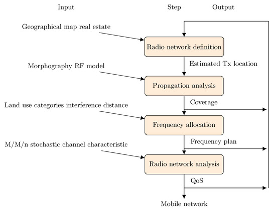
Figure 1.
Conventional approach to cellular network planning.
In ARPS, there is a possibility to improve this manual planning using a module called Automatic Cell Planning (ACP). Based on the documentation [10], it could improve the existing networks by tuning parameters that can easily be changed remotely such as antenna electrical tilt and power. Further, this module can optimize a network planning phase by (i) selecting antennas; (ii) modifying the antenna azimuth; (iii) setting the mechanical downtilt of the antenna; (iv) changing the antenna height; and (v) choosing sites from a list of candidate sites [10]. The variant provided by ARPS considers selecting sites (gNodeB locations), without the consideration of advanced aspects as is the expected customer throughput in the defined areas to be covered.
The whole idea of deploying or optimizing the network is shown in Figure 2. The provided solution is fully automated. That is an important advantage over the existing software solutions.
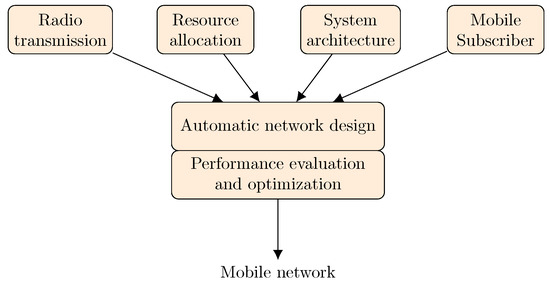
Figure 2.
Sophisticated network planning.
The proposed model has four aspects: (i) radio transmission (the transmission range, bidirectional/unidirectional, frequencies, etc.); (ii) resource allocation (the budget represented for the deployment); (iii) system architecture (types of gNodeB to use in the deployment, restricted places, etc.); and (iv) mobile subscriber (the expected number of users in the selected area and the expected average user traffic). Taking into account the parameters, we can compute the optimal gNodeB placement for the given area.
To solve such a task, we need to develop a mathematical model (see Section 2) and suitable implementation that will fit the above-mentioned automatic network design in an optimal way. Table 1 shows the terminology used in the remaining part of this paper adapted to the terms used in the literature.

Table 1.
Mapping mathematical terminology to communication networks terminology.
Automated wireless network design leads to a model formulated as Set Covering Problem (SCP) that belongs to the -complete class of problems [11]. Whereas the SCP model was more of a mathematical puzzle trying to find the smallest number of subsets, whose union covers the whole set of elements (the universe), its extensions encapsulate the essence of design in efficiently allocating facilities across geographic space. These extensions commonly deal with aspects such as location, facility type, thresholds, capacities and others. For example, the Capacitated Location Set Covering Problem with Equal Assignment (CLSCP-EA) [12], which is concerned with capacity consideration, is assigning capacities equally. It works as follows: let us consider three service centres which cover one customer location, in that case, the customer location capacities are distributed equally among these three service centres. Currently, the extensions of SCP are not usable for modern telecommunication networks since they are not taking into account the important aspects related to the network capacity, i.e., (i) direct assignment of customer location capacities straight to the service centre (in the wireless networks, this task is equal to assigning users throughput demands to particular gNodeB node); and (ii) considering the network-area capacity requirements including the considerations of the existing services (here, it means to keep the existing gNodeB nodes in the process of optimizing the network coverage, for further information see Section 1.1).
1.1. Literature Review
The literature review in this paper can be split into two parts. First, the models for location covering problems are presented since they represent the basic building blocks for our developed mathematical models. Secondly, we focus on the papers that are dealing with the gNodeB (or eNodeB, Base Transceiver Station (BTS) in older systems) deployment.
1.1.1. Location Covering Problems
Covering problems have been discussed for more than 50 years finding a wide area of applications [13,14,15,16,17,18,19,20,21,22,23] (Based on the Scopus database there were 4634 papers published on Set Covering Problem in the area of computer science or mathematics (5 November 2020). Since Scopus does not support multiple-word queries, such as set covering problem, the results may contain false positive matches).
It has a decisive role in the success of supply chains with applications including locating gas stations, schools, plants, landfills, police stations, design of sensor networks, etc. Currently, there exists a plethora of models that fall into the category of covering problems such as edge covering [24], vertex covering [25], capacitated vertex covering [26] and others. In this paper, the focus is especially given to the covering problems that are targeting the optimization of the network facilities locations in the selected areas.
For the goals stated in this paper, in regards to the optimization of static network infrastructure, the base covering model is LSCP together with its extensions. These were developed from the SCP model and, thus, share the same aspects such as its minimal computational complexity.
The three extensions of capacity-based LSCP can be considered: (i) CLSCP-CA; (ii) CLSCP-EA; (iii) Capacitated Location Set Covering Problem-System Optimal (CLSCP-SO). The first one concerns the use-case when the closest service centre is used for handling the requirements within the customer locations. The second one is concerned with the equal assignment of capacities over the accessible service centres and the third one is about service centre capacities that assign the fragmented capacities to the customer locations. In this fashion, an overview of related mathematical models for covering problems is shown in Table 2. For further mathematical model details, see the following publications [32,37,38,39,40,41,42,43,44,45]. Even if these models are dealing with capacities for location-based SCP, they are not applicable in 5G and beyond deployment since they do not take into account the fact that the user device requested capacity (bandwidth) could not be split over more than one gNodeB at the same time. Further, these models do not take into account interferences in any way. In our use-case, we need to consider the aspects such as wireless interference, direct (capacity) assignment of customer locations to a service centre and existing services in a given area.
Table 2.
An overview of core mathematical models for covering problems.
From the above-mentioned review, we deduce that the already proposed modifications of the SCP are not suitable for the use-case of optimization of network infrastructures. For that reason, the main contribution of this paper lies in the development of new mathematical models to provide a solution to the emerging scenario of 5G and beyond wireless deployments.
1.1.2. Base Station Optimization and Deployment
Since the deployment of gNodeB nodes is a very complex task, the papers published on that topic vary a lot (Based on the Scopus database, there were 4405 papers published on wireless networks deployment in the area of computer science, engineering or multidisciplinary sciences (5 November 2020)). The papers touching that topic are mostly focused on specific parts of the deployment. From the authors’ point of view, the papers are mostly targeting the problem of dynamically modifying the gNodeB parameters as-is: downtilt, the collection of three azimuths, mechanical downtilt, electrical downtilt, heigh of gNodeB and transmit power [46,47]. Further, the papers are targeting the deployment algorithms to determine the most suitable positions of gNodeB nodes. In [48], a pico gNodeB deployment problem was formulated as an additional task to meet the increasing data exchange requirements, which assures the performance of coverage and quality of services; besides, ref. [49] proposed several gNodeB deployment algorithms including region-based, grid-based and greedy algorithms to determine the most suitable positions of micro gNodeB nodes. However, these works only consider the impact of location, where other parameters that affect the performance indicators are not taken into consideration. Moreover, those algorithms optimize only one variable in each iteration and are performed in an exhaustive manner, which is inefficient with poor performance [47]. The overview of the recent literature in gNodeB optimization and deployment is shown in the Table 3. Additionally, the literature review of gNodeB deployment is presented in the following surveys in more detail [50,51,52,53,54,55,56,57,58,59,60,61].
Table 3.
An overview of recent papers targeting the deployment of gNodeB nodes.
In this paper, the target contribution is mainly on the gNodeB location optimization but, as opposed to the literature presented, we consider more aspects that are essential in the real-world scenarios.
1.2. Problem Formulation and Related Work
According to our previous work [65], the network infrastructure can be defined as the following graph. Assume that the network infrastructure contains m vertices (service centres), and n vertices (customer locations), and for each pair of vertices i (considered as service centres) and j (customer locations) their signal strength is given using a suitable propagation model (see more detailed discussion on the Equation (42)). In addition, is defined as the minimum signal strength which will be regarded as sufficient to establish the communication link between the service centres and customer location (these variables are described in more detail in Section 3).
Let us consider two finite sets I and J, where:
- I is the set of service centres ,
- J is the set of customer locations .
The aim was to determine which vertices must be used as service centres for each customer location to be covered by at least one of the centres and to minimize the number of operating centres. In other words, with respect to the targeted real-life scenario, we want to define a minimum number of gNodeB nodes while still providing coverage for all users in a given area.
Remark 1.
- 1.
- A condition necessary to solve the task is that all of the customer locations are reachable from at least one location where an operating service centre is considered.
- 2.
- Customer location j is reachable from vertex i, which is designated as an operating service centre if . If this inequality is not satisfied, vertex j is unreachable from i.
Here, means that vertex j has a signal with sufficient strength from the service centre i, means the opposite, and expresses the weights of service centres (since it is the minimization problem, the greater the weights are, the smaller the coefficient must be). If all the weights are set to 1 (i.e., all the centres are equally important), then we get a basic version of the set covering problem.
Similarly for decision variables , means that the service centre i is selected, while means that it is not selected. Then, the set covering problem can be described by the following mathematical model [38,65,66,67,68,69,70].
Minimise
Subject to
The objective function (1) represents the number of operating centres, constraint (2) means that each customer location is assigned to at least one operating service centre. Following that, the represents a threshold of service reachability.
To solve the above-described model, we have utilized an enhanced genetic algorithm as one of the possible solutions [65]. This was used for minimizing the number of schools in the selected area in Central Europe, but the theoretical concept was the same. However, in that work, we did not consider the capacity of service centres and the capacities potentially requested from customer locations. Therefore, in this paper, we propose the model and its implementation applied to optimizing wireless networks infrastructure while taking into account the capacity features mentioned.
1.3. Main Contribution
In this paper, we focus on the design of novel mathematical models for covering-based problems for the use-case of the infrastructure optimization in modern wireless networks. The developed models are the key enablers for the automatic base station deployment while building new networks as well as for the optimized location of currently deployed base stations. Our main contribution lies in the development of two mathematical models that deal with the task of direct capacity assignment and while considering the existing network infrastructure. These models are implemented and verified through prepared 5G networks datasets defining the common gNodeB parameter as well as the expected average throughput required by each user. Additionally, we prepared a dataset collected from the case study scenario covering the deployment of cellular infrastructure in the selected city district in Central Europe.
The remaining part of this paper is structured as follows. In Section 2, we introduce the newly created mathematical model for covering-based problems including direct capacity assignment. In Section 2.3, we discuss an extension for the capacity-based location problems with the consideration of the existing network infrastructure (i.e., already deployed gNodeB), which co-exists with the new one. The implementation perspective for the developed mathematical models, such as data representation and the whole computation concept, is described in more detail in Section 3. Finally, Section 4 introduces the results obtained through the numerical simulations and Section 5 is summarizing our main conclusions.
2. Models Developed for Network Coverage and Capacity Problems
As it was discussed in the Section 1.1, the original mathematical models for the location covering problems cannot be applied to our use-cases. We need to take into account the following two scenarios:
- deploying service centres to the new area or reconfiguration of the whole network,
- deploying additional service centres to the area, where service centres already exist, but do not provide sufficient network capacity.
Both of these scenarios need to consider the available capacities of service centres and required capacities from customer locations. These considerations are based on the fact that it is not possible to assign an unlimited number of customer locations (user equipment) to the service centres (gNodeB nodes) as the total cell to gNodeB capacity is capped. Especially, in 5G and beyond deployments, the number of connected devices is increasing rapidly due to the evolvability of IoT and other devices. For that reason, there is a need to effectively deploy gNodeB nodes and assign customer capacities. To deal with that issue, the new mathematical models considering gNodeB deployment with the required aspects are proposed.
Further, the variables and parameters used in the following mathematical models are denoted as follows:
- —capacity of service centre i,
- —the list of devices from customer location j that need a service centre,
- —customer from location j is assigned or is not assigned to service centre i,
- —expresses the weights of service centre i (in practice, it represents the gNodeB installation costs).
The above scenario is illustrated in Figure 3, where represents a service centre with given coverage range. represents customer location, where the colour indicates to which service centre that customer location is assigned.
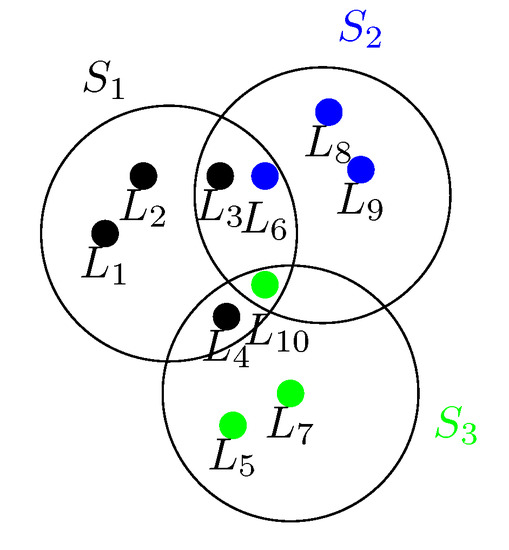
Figure 3.
The illustrated scenario where each customer location is assigned exactly to one service centre.
Based on the above assumptions, we formulate the models in Section 2.1 and Section 2.3.
2.1. Capacitated Network Area Coverage
Let us assume that each customer location is assigned directly to the one service centre with sufficient signal strength. This is guaranteed by Equation (4).
By Equation (5), each selected service centre must have its capacity sufficient for all the devices of customer locations that are assigned to it.
If a service centre is selected to be removed from the network infrastructure, none of the customer locations should be assigned to it, this is given by Equation (6).
All selected service centres must have a sufficient sum of their capacities to cover all devices (or facilities) in all customer locations.
This is guaranteed by constraints (7).
Now, we can summarize all the previous considerations in the following model.
Minimize
subject to:
A necessary precondition for finding a solution is that the sum of all capacities is sufficient to cover all demands, i.e., , with each customer having a reachable distance to at least one centre, i.e., .
This model is applicable especially in those use-cases in which we are deploying the gNodeB nodes to the new area or if we can rebuild the whole existing network. However, in many scenarios, we need to take into account the existing gNodeB nodes (existing services), for that reason, we have created the next model considering that use-case.
2.2. Wireless Interference Considerations
In wireless networks, it is essential to consider the signal interferences from service centres (gNodeB nodes) in the deployment. Assume that coverage cannot be provided from a single node. In our case, it is necessary to extend the model presented in Section 2.1 with additional objective and constraints to minimize the potential wireless interferences. Further in this section, we define that goal in the mathematical notation and discuss the benefits of using this extension.
If is the distance between centres i and j, then it is possible to solve this by: (i) an additional condition that, for all pairs of selected centres, will have a distance greater or equal than a certain threshold; or (ii) extending the objective function where the sum of mutual distances of selected centres will be maximised. The constraint for the first case can be expressed by the following equation.
The product in Equation (16) provides that this relation will be checked only for the selected pair of centres. However, since the previous equation is nonlinear, we replace the product of binary variables with the following linear equation.
Consider the second case. Then the problem changes to a multicriteria one. Both criteria can be aggregated by a scalarization procedure. Since the first criterion (number of selected centres) is minimizing and the second criterion (sum of mutual distances) is maximizing, the second criterion will be considered with a negative sign. In addition, it is necessary to unify both criteria into the same range of values from the interval .
Equation (8) for the objective function changes as follows:
Instead of min in the objective function, and the following additional constraints may be used
Of course, even here, the degree of importance of both sub-criteria can be expressed by weights, , , which leads to Equation (22).
By including both approaches, the final model is as follows:
Minimize
subject to:
Using this model extension, we reduce the potential wireless interference by deploying service centers (gNodeB nodes) with the greatest possible distance between them. In practice, usually specific (gNodeB) cells communicate at a different frequency, thus limiting interference at locations that are covered by multiple gNodeB nodes. By reducing the number of customer locations that are covered by more gNodeB nodes, we reduce the potential wireless interferences. This can also be achieved with a modification of the parameters of the gNodeB nodes (transmission power, etc.); however, it is advisable to consider this problem also in the process of selecting the appropriate positions for deployment.
2.3. Capacitated Network Area Coverage with Existing Services
The problems of existing services were discussed widely in the [71]. Here, the discussion was issued in the context of covering of fire brigade locations through an extension of the MLCP. Since the existing facilities may prove to be spatially inefficient, the systematic analysis is essential for evaluating both short and long-term costs. In the context of this paper, the existing services are an important part of the deployment since it is not a trivial or inexpensive task of changing the position of the existing gNodeB nodes. In most scenarios, we need to extend, enhance or replace the existing service centres by new service centre configurations. In addition to the previous model, we had to add another constraint that will add the existing services to the solution explicitly as follows:
where represents the set of existing service centres.
The whole extended model of Section 2 would change as follows for the use case of deployment in the area with existing services.
Minimize
subject to:
where is the additional cost of building a new service centre as compared to keeping an existing one. The objective function may be modified in the same way as in Equation (22), considering the existing nodes. Interference must be eliminated for all pairs of newly added centres and also for new and existing centre, which is satisfied by Equations (38) and (39). The other parameters are the same as in the model provided in Section 2.1, and for its solvability, the same assumptions must be satisfied.
3. Computational Concept
The whole computational concept can be divided into two steps: (i) prediction of the radio channel conditions between service centres and customer locations using selected propagation model; and (ii) employment of the developed models to find optimal locations to deploy service centres.
An important note here is that, before the actual deployment of the proposed models, it is appropriate to consider whether the network infrastructure can be optimized by changing the parameters of gNodeB nodes only. With this in mind, we recommend testing methods aimed at optimizing the gNodeB parameters of the network before deploying these models [47]. If it is not possible to meet the requirements of end-users by simply changing the parameters of gNodeB nodes, it is suitable to apply the proposed computational model.
3.1. Propagation Models
The relations between service centres and customer locations are based on the final signal strength. Using this approach we will get the relation between each gNodeB node and each selected area (e.g., each user location). Here, we assume that each gNodeB node is configured at its best for the given position to cover as many locations as possible [72,73]. Further, this prediction has to be done depending on the deployment scenario (urban, suburban, rural area). For example, for urban/suburban areas the suitable path loss prediction models are (i) Okumura-Hata Model; (ii) Stanford University Interim (SUI) Model; and (iii) Cost 231 Hata Model. From that list, for 5G and beyond deployments (in urban and suburban areas) the SUI Model seems promising [74] for frequencies ranging from 2 to 11 GHz. This model is expressed by the following formula:
where d is the distance between the gNodeB node and the receiving antenna, = 100 [74,75], is the path-loss exponent, is the correction for frequency above 2 GHz, is the correction for receiving antenna height, s is the correction for shadow fading due to trees and other clutter and is the wavelength [74]. The other parameters are defined as:
where is the gNodeB node height above ground in meters, and are constants that vary with terrain.
3.2. Employment of Developed Models
Based on the selected propagation model, we construct the initial matrix representing the relation between service centres and customer locations. This initial matrix is represented as a matrix (rather than linked list) since it brings the benefit of a fast access () to particular rows and columns. The process of data representation and manipulation is shown in Example 1.
In Example 1, we define a as | . It is designed based on the specification of Reference Signal Received Power Categories (RSRPC) for Sub-6 GHz 5G cellular service mode that is briefly shown in Table 4 [76,77].
Table 4.
Reference Signal Received Power Categories for Sub-6 GHz 5G service mode [76,77].
Here, we see that, if the signal power is −80 dBm or higher, then the signal is excellent, while when the signal power drops to −100 dBm and lower, it becomes impossible to establish or keep the wireless connection.
Example 1.
The following matrix expresses the relationship between the service centres and customer locations. Rows represent service centres and columns are related to the customer locations.
Depending on , the reachability matrix would be as follows:
Based on the reachability matrix, the matrix including customer locations capacities would be as follows (the number in round brackets of S means the maximal capacity of the service centre and the number in a particular column means the requested capacity for the customer location):
Here, we generally use non-unitary variables, but you can take this number to correspond to the network throughput demanded by a given customer location, or it can be a combination of multiple parameters.
If we need to consider the existing services from models described in Section 2.3, we can do this in the same way as we did in [65] for the necessary services. This refers to adding dummy columns or directly setting to 1.
The whole concept of producing the optimal solution is presented in Algorithm 1.
The computational concept for the developed models is shown in Figure 4.
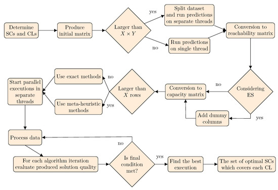
Figure 4.
The basic concept of producing the optimal solution (SC: service centre, CL: customer location and ES: existing services).
The decision node for an initial matrix represents the condition that if the initial matrix size is larger than , where X is the number of rows and Y is the number of columns (the value depends on the computation environment, where the run will be invoked), we should take into account parallel processing being used. For example, if the matrix has a dimension of , the application needs to calculate the prediction model 75,000,000 times. The parallel processing for that can be achieved by spliting the dataset into separate threads. Then the process waits for each thread to finish its computation to merge the results into the initial matrix. The next key decision is to consider the number of rows (X). In that case, we know from previous sections that this problem has at least the complexity of . For that reason, for more than 60 rows (X > 60) we can expect that the duration of computation with exact methods, on a typical desktop computer with 3 GHz processor, will be in the range of years [65]. The common exact methods used for calculations with X < 60 are: (i) branch-and-bound [78,79,80,81]; and (ii) removal algorithm [82]. These exact methods are commonly applied together with relaxations algorithms that reduce the size of SCP-based problems. The examples of such relaxations are: (i) Dual LP; (ii) Prima-Dual; (iii) Lagrangian relaxation; and (iv) Surrogate relaxation [83,84,85]. In the case of large datasets (i.e., X > 60), the meta-heuristic needs to be applied to provide a suitable solution in a reasonable time. The meta-heuristic algorithms are the class of computational methods used for optimization problems, which do not guarantee the optimal but acceptable solution. Since meta-heuristic methods contain a broad range of algorithms, we need to provide a survey on what are the options available at present. Following the literature review, we can divide the meta-heuristic algorithms into three categories: (i) swarm-based algorithms; (ii) evolution-based algorithms; and (iii) hybrid algorithms. Each of these categories contains a plethora of algorithms. The commonly used algorithms for the first category are Ant Colonies Optimization (ACO) [86], Harmony Search (HS) [87], Particle Swarm Optimization (PSO) [88], Artificial Bee Colony (ABC) [89], Gravitational Search Algorithm (GSA) [90], Firefly Algorithm (FA) [91], Teaching Learning Algorithm (TLA) [92], Chemical Reaction Optimization (CRO) [93], Water Cycle Algorithm (WCA) [94]. For the second category, there are Genetic Algorithm (GA), Differential Evolution (DE) [95], evolutionary programming and evolutionary strategies [96], Differential Search Algorithm (DSA) [97], and for the last category we can mention ant colony optimization with variable neighbourhood search and genetic algorithms with variable neighbourhood search. We see that, until now, a lot of meta-heuristic algorithms have been developed. The experiments could be done using any of these, because of the No free lunch theorem [98], it is not possible to expect that any of these algorithms can provide an ideal solution for all the use-cases and datasets. However, for SCP-based problems, it is quite common to employ evolution-based algorithms [99,100,101,102].
Despite the computational complexity presented in Section 3.3, we implemented it in the GAMS optimization tool, as mentioned above, and successfully solved instances with thousands of rows and columns. The results of calculations for such large instances were received in tens of minutes on regular desktop computer (processor: Intel(R) Core(TM) i7-7700 CPU @ 3.60 GHz 3.60 GHZ; installed memory (RAM): 16.0 GB; and 64-bit operating system). Since the calculation by GAMS uses deterministic heuristic, there is no need for statistical evaluation of calculations based on dozens of runs of stochastic heuristic methods.
Further, on the results from the presented models, we suggest using additional optimization to tune the gNodeB parameters (power, downtilt, height, etc.) to provide the optimal gNodeB configurations. To tune these parameters, we suggest considering the multi-objective genetic algorithm presented in [47].
| Algorithm 1 The algorithm representing the whole computational concept to get the best locations to deploy service centres (gNodeB) nodes. |
|
3.3. Model Computational Complexity Considerations
Generally, it is known that the SCP is NP-hard [103].
The size of the search space is determined by the number of all possible selections of centres. For n centres, according to the binomial theorem, it is equal to
4. Numerical Simulations and Results Discussion
The mathematical models presented are targeting two deployment scenarios, the first one is to deploy the gNodeB nodes to the area without the existing gNodeB nodes, i.e., new deployment, and the second one is to deploy additional gNodeB nodes to the area with the existing gNodeB nodes, i.e., to increase the overall network capacity.
For the first scenario, we prepared self-developed datasets to use the mathematical model for the deployment without the existing infrastructure for different scenarios (urban, suburban and rural). For the second one, we use the mathematical model that takes into account the existing infrastructure, here the input values have been obtained from publicly available data (about users, gNodeB nodes, etc.) in the selected district of Central Europe.
4.1. gNodeB Parameters Settings
To prepare the datasets, we need to consider the parameters taking into account the expected user connection growth, maximal available throughput (capacity) of gNodeB node, and gNodeB coverage range for selected the deployment use-cases. For the sake of simplification, we consider that a single gNodeB represents a single mobile cell. All the parameters are further discussed in the next paragraphs.
To estimate the expected connection growth and required throughput, we used the parameters from the white paper [5] from Cisco company and the 5G reference guide for network operators [104]. In [5], we see that the fastest-growing device and connections category is Machine-to-Machine (M2M) (see Figure 5) that can grow to reach 14.7 billion connections by 2023. Here, it is important to track the changing mix of devices and connections and growth in multi-device ownership as it affects traffic patterns. Video devices, in particular, can have a multiplier effect on traffic. An Internet-enabled High Definition (HD) television that draws two hours of content per day from the Internet would generate, on average, as much Internet traffic as an entire household today. The impact of devices with video on the network traffic is more pronounced because of the introduction of Ultra-High-Definition (UHD), or 4K, video streaming. The expected user thresholds are for Downlink (DL) 100 Mbit/s and for Uplink (UL) it is 50 Mbit/s. This high data rate demanded by end-users is based on the situation that in the 5G systems, there is a high expectation for emerging high-end user applications such as AR or VR, that require data rates in the range of several hundreds of Mbit/s [5,104]. Based on this information, we used the values from [5] that expect the significant growth of M2M devices and other devices in 2023 that can produce a workload close to 43.9 Mbit/s. This value was estimated in the [5,104] based on the wide usage of AR, VR and such applications. In the presented scenario, it represents the upper limit that the network operator will allocate for one user. We used that value to design the network to handle such borderline scenario [104].
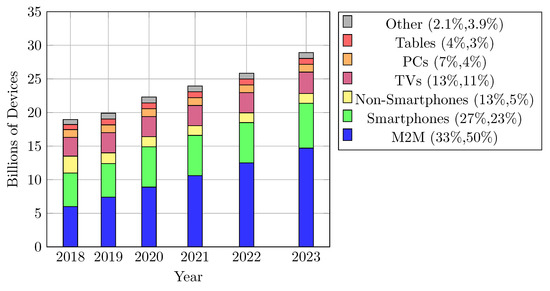
Figure 5.
Global device and connection growth.
On the other hand, based on the specification presented in [105], the expected capacity limits of a single gNodeB node are as follows: (i) DL peak data rate 20 Gbit/s and; (ii) UL peak data rate is 10 Gbit/s. These requirements are further specified for selected deployment use-cases (urban, suburban, rural) [106]. In practice, the capacity of gNodeB node is dependent on a variety of configuration parameters as-is: hardware setup, class of radio interface, duplex mode, number of sector carriers/baseband unit, number of users/baseband unit, number of users/sector carrier, data radio bearers, scheduling entities per slot DL/UL—cell, maximum sector carrier bandwidth, maximum throughput per connected user DL/UL, maximum throughput per radio node DL/UL and Single User (SU) Multiple-Input Multiple-Output (MIMO) layers. All of these can be further optimized based on the actual requirements after the deployment is complete. For the sake of generalization, the average base station coverage range (cell range) is most commonly set to 0.5 km in urban, 1 km in suburban and 8 km in rural areas [107]. Further, in the numerical simulations, we used the parameters to set the SUI model that is typically used in practical applications. The settings for each gNodeB node were as follows a = 4, , , ranging from 5 to 35 m, f was under 5 GHz, , and s were calculated using the antenna height and frequency parameters).
The summarized list of parameters of gNodeB and users is shown in Table 5.
Table 5.
Summarized list of parameters based on the deployment use-case.
4.2. Simulation of Different Deployment Scenarios
Based on the parameters set as presented in Table 5, for each scenario (urban, susburban, rural) we created five datasets. Within them, we considered various numbers of theoretical candidate locations given an identical number of users and total coverage area. The simulations carried out made it possible, in a reasonable time, to achieve the results presented in Table 6. For these simulations, the model presented by Equations (23)–(30) was used without extending the objective function, which might be an interesting problem for further research. Interferences were reduced by Equation (28).
Table 6.
Results of different deployment scenarios.
In that table, it is clearly shown that the area size is not the biggest problem for the gNodeB deployment, as opposed to the number of users and their required throughput which is the main aspect that needs to be considered for the 5G and beyond deployments. In addition, it is shown that even if the rural use-case contains the same number of users as the urban area, the number of the necessary gNodeB to cover the area is smaller. This is especially due to the larger number of theoretically available locations to deploy gNodeB on which the software can find better combinations of gNodeB nodes to cover the whole area to meet the given requirements. The theoretical candidate locations were generated randomly based on the assumption that larger areas should have better options to select locations to deploy gNodeB nodes.
For the computational concept, we consider that, theoretically, the base station could be deployed on every possible place (see Figure 6) and then the software will produce the combination of the gNodeB nodes locations that is optimal for the considered deployment, based on the selected aspects.
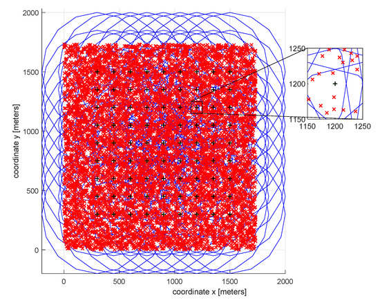
Figure 6.
Initial theoretical distribution of possible locations of gNodeB in an urban area (red cross symbol represents user; black plus symbol represents gNodeB; and blue circle represents the gNodeB coverage radius).
In this visualization, it is shown that, in the case of an urban area, users are spread throughout the area. It is further shown here that 81 possible locations for gNodeB node deployment were originally considered and, of these, an optimal combination of 19 gNodeB nodes was found. The calculated solution covers the whole area meeting the specified requirements (gNodeB capacities, expected throughput from the user and range of gNodeB). If the area changes significantly, e.g., some areas may be closed and users may move to another district, the only essential process to do is to provide updated input parameters for our models.
The optimal combination of gNodeB nodes is shown in Figure 7.
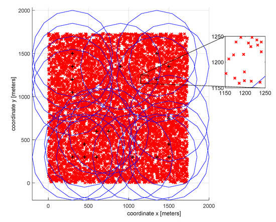
Figure 7.
The final deployment solution for gNodeB on an urban area (red cross symbol represents user; black plus symbol represents gNodeB candidate location; and blue circle represents the gNodeB coverage radius).
4.3. Simulations Utilizing Dataset From District in Central Europe
In this case study scenario, we consider the use-case of adding new gNodeB nodes to the area in the city of Prague. Here, we assume that, within 3 years, the network traffic will approximately double based on the information provided in [5]. The area that was selected for that network infrastructure reconfiguration represents a typical mixed-urban environment consisting of residential areas, forests, industrial areas, etc. The list of available gNodeB nodes in the selected area consists of 75 already deployed (gNodeB/eNodeB/BTS) nodes with the peak capacity of 1 Gb/s UL; 500 Mb/s DL for each node. This information can be extracted from a freely available data source at https://www.gsmweb.cz.
The next step was to select particular areas to cover and predict the signal strength and network traffic in those areas. The traffic had to be predicted based on the type of location since it is likely to be higher in an industry area than in a forest. First, we need to predict the signal strength in relation to each gNodeB node and each selected area (e.g., each user location). This prediction was based on the deployment use-case that is in a particular urban/suburban area. For that reason, the SUI propagation model was chosen.
To simulate the model considering the existing gNodeB nodes the district Prague 11 was selected. This district has a total of 68,839 residents [108] (some of the residents are commuting to another district and some of them visit the district during the day, but for simplicity, we consider the size of both groups equal). Based on that data and the theoretical locations of new gNodeB nodes, we computed the optimal locations of the base stations to satisfy the new requirements due to an increasing number of connected devices with high traffic (HD video, VR, AR and others). In addition, for the computation, we expected that all the existing gNodeB nodes have a total cell capacity of 30 Gbit/s per gNodeB with a cell coverage radius of 1 km. The additional parameters for that computation are shown in Table 7.
Table 7.
Prague 11 deployment use-case.
Using these assumptions, the dataset from the Prague 11 district was processed. The result is shown in Figure 8, where the existing gNodeB nodes are marked as blue circles and the newly added gNodeB nodes are marked as black circles. In this figure, it is shown that it would be essential to add an additional 31 gNodeB nodes to provide the network infrastructure that can deal with the increasing traffic demand.
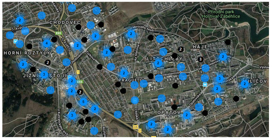
Figure 8.
Selected gNodeB deployment with the new requirements, the numbers in the circles indicate the number of gNodeB nodes in the particular location.
Based on that computation, we see that, for 5G and beyond (6G), the network operators will need to significantly modify the network infrastructure to be able to handle the increased network traffic and here our models will provide a value that can be of major use.
In practice, the process of adding gNodeB nodes is not appropriate, and usually not even possible on a large scale. This is due to the gNodeB building process that involves a number of steps, both legal and structural. For that reason, it is advisable to add gNodeB nodes iteratively based on the current growth of network traffic with a certain reserve. In both our models, this can be expressed by just changing the input data values, e.g., multiplying the demanded user throughput to include the new applications in 5G.
5. Conclusions
This paper introduces newly developed mathematical models that deal with the automatic network infrastructure design. These models were developed for two use-cases and implemented in the GAMS optimization tool. In the first case, the model enables the deployment of gNodeB nodes in a new area (without any existing infrastructure), and in the second case, it adds additional gNodeB nodes to the area with an existing, but not sufficient, infrastructure.
Both models take into account important aspects such as the required user throughput that is rapidly growing these days in 5G networks as well as the aspect of deploying the gNodeB nodes that need to coexist with the existing infrastructure. These models can be used to improve the network design of the existing software solutions such as Atoll Radio Planning Software to do the network planning more efficiently. Further, we provide a data representation and computation concept to be able to implement it in an optimal way. Based on that, the models are validated through simulations provided for each deployment scenario (urban, suburban, rural area). The results of the simulations prove that these models are well-designed and can optimize the network in a significant manner. Furthermore, these simulations show that to deploy emerging wireless networks on a full scale with all the applications as is AR, VR and others, the network infrastructures have to be significantly enhanced.
For future research, we will focus on the employment of a swarm of drones as flying on-demand gNodeB nodes to dynamically cover the selected areas in critical scenarios (e.g., public safety, and natural disasters), which typically require considering additional aspects.
Author Contributions
Writing-original draft preparation, P.S.; software, P.S., M.S.; formal analysis, P.S., M.S.; visualization, P.S.; writing-review and editing, J.H., M.S.; supervision, J.H.; funding acquisition, J.H. All authors have read and agreed to the published version of the manuscript.
Funding
This research was funded by Brno University of Technology Program under Grant BD182018001.
Acknowledgments
Research described in this paper was financed by the Brno University of Technology Program under Grant BD182018001. For the research, infrastructure of the SIX Center was used.
Conflicts of Interest
The authors declare no conflict of interest. The funders had no role in the design of the study; in the collection, analyses, or interpretation of data; in the writing of the manuscript, or in the decision to publish the results.
References
- Qamar, F.; Hindia, M.; Dimyati, K.; Noordin, K.A.; Majed, M.B.; Abd Rahman, T.; Amiri, I.S. Investigation of future 5G-IoT millimeter-wave network performance at 38 GHz for urban microcell outdoor environment. Electronics 2019, 8, 495. [Google Scholar] [CrossRef]
- Aranda, D.A.; Fernández, L.M.M.; Stantchev, V. Integration of Internet of Things (IoT) and Blockchain to increase humanitarian aid supply chains performance. In Proceedings of the 2019 5th International Conference on Transportation Information and Safety (ICTIS), Liverpool, UK, 14–17 July 2019; pp. 140–145. [Google Scholar]
- Al-Yasir, Y.I.; Ojaroudi Parchin, N.; Abd-Alhameed, R.A.; Abdulkhaleq, A.M.; Noras, J.M. Recent progress in the design of 4G/5G reconfigurable filters. Electronics 2019, 8, 114. [Google Scholar] [CrossRef]
- Shukla, S.; Hassan, M.F.; Khan, M.K.; Jung, L.T.; Awang, A. An analytical model to minimize the latency in healthcare internet-of-things in fog computing environment. PLoS ONE 2019, 14, e0224934. [Google Scholar] [CrossRef]
- Cisco Visual Networking Index. Cisco Visual Networking Index: Forecast and Trends, 2018–2023; White Papper; Cisco Visual Networking Index: San Jose, CA, USA, 2020. [Google Scholar]
- Bansal, G.; Jain, A.K.; Mishra, T. 5G Technology and Their Challenges. J. Adv. Database Manag. Syst. 2019, 6, 1–7. [Google Scholar]
- Shen, C.; Yun, M.; Arora, A.; Choi, H.A. Efficient mobile base station placement for first responders in public safety networks. In Proceedings of the Future of Information and Communication Conference, San Francisco, CA, USA, 14–15 March 2019; pp. 634–644. [Google Scholar]
- <i>Rios, R. 5G Network Planning and Optimisation Using Atoll. Master’s Thesis, Universitat Politècnica de Catalunya, Barcelona, Spain, 2019. [Google Scholar]
- Tutschku, K. Demand-based radio network planning of cellular mobile communication systems. In Proceedings of the Conference on Computer Communications. Seventeenth Annual Joint Conference of the IEEE Computer and Communications Societies. Gateway to the 21st Century, San Francisco, CA, USA, 29 March–2 April 1998; Volume 3, pp. 1054–1061. [Google Scholar]
- Mohammed, M.E.; Bilal, K.H. LTE Radio Planning Using Atoll Radio Planning and Optimization Software. Int. J. Sci. Res. 2014, 3, 1460. [Google Scholar]
- Karp, R.M. Reducibility among combinatorial problems. In Complexity of Computer Computations; Springer: Berlin/Heidelberg, Germany, 1972; pp. 85–103. [Google Scholar]
- Dembski, W.A.; Marks, R.J. Bernoulli’s principle of insufficient reason and conservation of information in computer search. In Proceedings of the 2009 IEEE International Conference on Systems, Man and Cybernetics, San Antonio, TX, USA, 1–14 October 2009; pp. 2647–2652. [Google Scholar]
- Toregas, C. A Covering Formulation for the Location of Public Facilities. Ph.D. Thesis, Cornell University, Ithaca, NY, USA, 1970. [Google Scholar]
- Sridharan, R. The capacitated plant location problem. Eur. J. Oper. Res. 1995, 87, 203–213. [Google Scholar] [CrossRef]
- Church, R.L.; Gerrard, R.A. The multi-level location set covering model. Geogr. Anal. 2003, 35, 277–289. [Google Scholar] [CrossRef]
- Cardei, M.; Du, D.Z. Improving wireless sensor network lifetime through power aware organization. Wirel. Netw. 2005, 11, 333–340. [Google Scholar] [CrossRef]
- Abrams, Z.; Goel, A.; Plotkin, S. Set k-cover algorithms for energy efficient monitoring in wireless sensor networks. In Proceedings of the 3rd International Symposium on Information Processing in Sensor Networks, Berkeley, CA, USA, 26–27 April 2004; pp. 424–432. [Google Scholar]
- Jeong, I.J. An optimal approach for a set covering version of the refueling-station location problem and its application to a diffusion model. Int. J. Sustain. Transp. 2017, 11, 86–97. [Google Scholar] [CrossRef]
- Maher, S.J.; Murray, J.M. The unrooted set covering connected subgraph problem differentiating between HIV envelope sequences. Eur. J. Oper. Res. 2016, 248, 668–680. [Google Scholar] [CrossRef]
- Davoodi, S.M.R.; Goli, A. An integrated disaster relief model based on covering tour using hybrid Benders decomposition and variable neighborhood search: Application in the Iranian context. Comput. Ind. Eng. 2019, 130, 370–380. [Google Scholar] [CrossRef]
- Vianna, S.S. The set covering problem applied to optimisation of gas detectors in chemical process plants. Comput. Chem. Eng. 2019, 121, 388–395. [Google Scholar] [CrossRef]
- Basciftci, B.; Ahmed, S.; Shen, S. Distributionally robust facility location problem under decision-dependent stochastic demand. Eur. J. Oper. Res. 2020, in press. [Google Scholar] [CrossRef]
- Chauhan, D.; Unnikrishnan, A.; Figliozzi, M. Maximum coverage capacitated facility location problem with range constrained drones. Transp. Res. Part Emerg. Technol. 2019, 99, 1–18. [Google Scholar] [CrossRef]
- Murty, K.G.; Perin, C. A 1-matching blossom-type algorithm for edge covering problems. Networks 1982, 12, 379–391. [Google Scholar] [CrossRef]
- Dinur, I.; Safra, S. On the hardness of approximating minimum vertex cover. Ann. Math. 2005, 162, 439–485. [Google Scholar] [CrossRef]
- Guha, S.; Hassin, R.; Khuller, S.; Or, E. Capacitated vertex covering. J. Algorithms 2003, 48, 257–270. [Google Scholar] [CrossRef]
- Berge, C. Two theorems in graph theory. Proc. Natl. Acad. Sci. USA 1957, 43, 842. [Google Scholar] [CrossRef]
- Church, R.R.C. The maximal covering location model. Pap. Reg. Sci. Assoc. 1974, 32, 101–118. [Google Scholar] [CrossRef]
- Plane, D.R.; Hendrick, T.E. Mathematical programming and the location of fire companies for the Denver fire department. Oper. Res. 1977, 25, 563–578. [Google Scholar] [CrossRef]
- Schilling, D.; Elzinga, D.J.; Cohon, J.; Church, R.; ReVelle, C. The Team/Fleet models for simultaneous facility and equipment placement. Transp. Sci. 1979, 13, 163–175. [Google Scholar] [CrossRef]
- Margules, C.R. Conservation evaluation in practice. In Wildlife Conservation Evaluation; Springer: Berlin/Heidelberg, Germany, 1986; pp. 297–314. [Google Scholar]
- Current, J.R.; Storbeck, J.E. Capacitated covering models. Environ. Plan. Plan. Des. 1988, 15, 153–163. [Google Scholar] [CrossRef]
- Revelle, C.; Hogan, K. The maximum reliability location problem and α-reliablep-center problem: Derivatives of the probabilistic location set covering problem. Ann. Oper. Res. 1989, 18, 155–173. [Google Scholar] [CrossRef]
- Gerrard, R.A.; Church, R.L. Closest assignment constraints and location models: Properties and structure. Locat. Sci. 1996, 4, 251–270. [Google Scholar] [CrossRef]
- Berman, O.; Krass, D. The Generalized Maximal Covering Location Problem. Comput. Oper. Res. 2002, 29, 563–581. [Google Scholar] [CrossRef]
- Hong, S.; Kuby, M. A threshold covering flow-based location model to build a critical mass of alternative-fuel stations. J. Transp. Geogr. 2016, 56, 128–137. [Google Scholar] [CrossRef]
- Melo, M.T.; Nickel, S.; Saldanha-Da-Gama, F. Facility location and supply chain management—A review. Eur. J. Oper. Res. 2009, 196, 401–412. [Google Scholar] [CrossRef]
- Farahani, R.Z.; Asgari, N.; Heidari, N.; Hosseininia, M.; Goh, M. Covering problems in facility location: A review. Comput. Ind. Eng. 2012, 62, 368–407. [Google Scholar] [CrossRef]
- Church, R.L.; Murray, A. Location Covering Models; Springer: Berlin/Heidelberg, Germany, 2018. [Google Scholar]
- Brimberg, J.; Drezner, Z. A location–allocation problem with concentric circles. IIE Trans. 2015, 47, 1397–1406. [Google Scholar] [CrossRef]
- Boonmee, C.; Arimura, M.; Asada, T. Facility location optimization model for emergency humanitarian logistics. Int. J. Disaster Risk Reduct. 2017, 24, 485–498. [Google Scholar] [CrossRef]
- Eiselt, H.A.; Marianov, V. Location modeling for municipal solid waste facilities. Comput. Oper. Res. 2015, 62, 305–315. [Google Scholar] [CrossRef]
- Sitepu, R.; Puspita, F.M.; Romelda, S.; Fikri, A.; Susanto, B.; Kaban, H. Set covering models in optimizing the emergency unit location of health facility in Palembang. J. Physics: Conf. Ser. 2019, 1282, 012008. [Google Scholar] [CrossRef]
- García, S.; Marín, A. Covering location problems. In Location Science; Springer: Berlin/Heidelberg, Germany, 2015; pp. 93–114. [Google Scholar]
- Berman, O.; Huang, R. The minimum weighted covering location problem with distance constraints. Comput. Oper. Res. 2008, 35, 356–372. [Google Scholar] [CrossRef]
- Mattos, D.I.; Bosch, J.; Olsson, H.H.; Dakkak, A.; Bergh, K. Automated optimization of software parameters in a long term evolution radio base station. In Proceedings of the 2019 IEEE International Systems Conference (SysCon), Orlando, FL, USA, 8–11 April 2019; pp. 1–8. [Google Scholar]
- Dai, L.; Zhang, H. Propagation-Model-Free Base Station Deployment for Mobile Networks: Integrating Machine Learning and Heuristic Methods. IEEE Access 2020, 8, 83375–83386. [Google Scholar] [CrossRef]
- Yigitel, M.A.; Incel, O.D.; Ersoy, C. Dynamic BS topology management for green next generation HetNets: An urban case study. IEEE J. Sel. Areas Commun. 2016, 34, 3482–3498. [Google Scholar] [CrossRef]
- Sui, X.; Zhang, H.; Lv, Y. Coverage performance analysis of grid distribution in heterogeneous network. In Proceedings of the 2017 IEEE 17th International Conference on Communication Technology (ICCT), Chengdu, China, 27–30 October 2017; pp. 1424–1428. [Google Scholar]
- Foukas, X.; Patounas, G.; Elmokashfi, A.; Marina, M.K. Network slicing in 5G: Survey and challenges. IEEE Commun. Mag. 2017, 55, 94–100. [Google Scholar] [CrossRef]
- Mukherjee, A.; Keshary, V.; Pandya, K.; Dey, N.; Satapathy, S.C. Flying ad hoc networks: A comprehensive survey. In Information and Decision Sciences; Springer: Berlin/Heidelberg, Germany, 2018; pp. 569–580. [Google Scholar]
- Chen, H.; Mo, Y.; Qian, Q.; Xia, P. Research on 5G Wireless Network Deployment in Tourist Cities. In Proceedings of the 2020 International Wireless Communications and Mobile Computing (IWCMC), Limassol, Cyprus, 15–19 June 2020; pp. 398–402. [Google Scholar]
- Kenyeres, M.; Kenyeres, J. Synchronous Distributed Consensus Algorithms for Extrema Finding with Imperfect Communication. In Proceedings of the 2020 IEEE 18th World Symposium on Applied Machine Intelligence and Informatics (SAMI), Herlany, Slovakia, 23–25 January 2020; pp. 157–164. [Google Scholar]
- Ganame, H.; Yingzhuang, L.; Ghazzai, H.; Kamissoko, D. 5G Base Station Deployment Perspectives in Millimeter Wave Frequencies Using Meta-Heuristic Algorithms. Electronics 2019, 8, 1318. [Google Scholar] [CrossRef]
- Han, F.; Zhao, S.; Zhang, L.; Wu, J. Survey of strategies for switching off base stations in heterogeneous networks for greener 5G systems. IEEE Access 2016, 4, 4959–4973. [Google Scholar] [CrossRef]
- Xu, X.; Saad, W.; Zhang, X.; Xu, X.; Zhou, S. Joint deployment of small cells and wireless backhaul links in next-generation networks. IEEE Commun. Lett. 2015, 19, 2250–2253. [Google Scholar] [CrossRef]
- Kenyeres, M.; Kenyeres, J. Distributed Network Size Estimation Executed by Average Consensus Bounded by Stopping Criterion for Wireless Sensor Networks. In Proceedings of the 2019 International Conference on Applied Electronics (AE), Pilsen, Czech Republic, 10–11 September 2019; pp. 1–6. [Google Scholar]
- Cacciapuoti, A.S.; Caleffi, M.; Masone, A.; Sforza, A.; Sterle, C. Data Throughput Optimization for Vehicle to Infrastructure Communications. In New Trends in Emerging Complex Real Life Problems; Springer: Berlin/Heidelberg, Germany, 2018; pp. 93–101. [Google Scholar]
- González-Brevis, P.; Gondzio, J.; Fan, Y.; Poor, H.V.; Thompson, J.; Krikidis, I.; Chung, P.J. Base station location optimization for minimal energy consumption in wireless networks. In Proceedings of the 2011 IEEE 73rd Vehicular Technology Conference (VTC Spring), Yokohama, Japan, 15–18 May 2011; pp. 1–5. [Google Scholar]
- Valavanis, I.K.; Athanasiadou, G.; Zarbouti, D.; Tsoulos, G.V. Base-station location optimization for LTE systems with genetic algorithms. In Proceedings of the 20th European Wireless Conference, Barcelona, Spain, 14–16 May 2014; pp. 1–6. [Google Scholar]
- Kenyeres, M.; Kenyeres, J. Average Consensus over Mobile Wireless Sensor Networks: Weight Matrix Guaranteeing Convergence without Reconfiguration of Edge Weights. Sensors 2020, 20, 3677. [Google Scholar] [CrossRef]
- Teague, K.; Abdel-Rahman, M.J.; MacKenzie, A.B. Joint base station selection and adaptive slicing in virtualized wireless networks: A stochastic optimization framework. In Proceedings of the 2019 International Conference on Computing, Networking and Communications (ICNC), Honolulu, HI, USA, 18–21 February 2019; pp. 859–863. [Google Scholar]
- Tayal, S.; Garg, P.; Vijay, S. Optimization Models for Selecting Base Station Sites for Cellular Network Planning. In Applications of Geomatics in Civil Engineering; Springer: Berlin/Heidelberg, Germany, 2020; pp. 637–647. [Google Scholar]
- Afuzagani, D.; Suyanto, S. optimizing BTS Placement Using Hybrid Evolutionary Firefly Algorithm. In Proceedings of the 8th International Conference on Information and Communication Technology (ICoICT), Yogyakarta, Indonesia, 24–26 June 2020; pp. 1–5. [Google Scholar]
- Seda, P.; Mark, M.; Su, K.; Seda, M.; Hosek, J.; Leu, J. The Minimization of Public Facilities With Enhanced Genetic Algorithms Using War Elimination. IEEE Access 2019, 7, 9395–9405. [Google Scholar] [CrossRef]
- Beasley, J.E.; Chu, P.C. A genetic algorithm for the set covering problem. Eur. J. Oper. Res. 1996, 94, 392–404. [Google Scholar] [CrossRef]
- Crawford, B.; Soto, R.; Cuesta, R.; Paredes, F. Application of the artificial bee colony algorithm for solving the set covering problem. Sci. World J. 2014, 2014, 189164. [Google Scholar] [CrossRef] [PubMed]
- Lanza-Gutierrez, J.M.; Crawford, B.; Soto, R.; Berrios, N.; Gomez-Pulido, J.A.; Paredes, F. Analyzing the effects of binarization techniques when solving the set covering problem through swarm optimization. Expert Syst. Appl. 2017, 70, 67–82. [Google Scholar] [CrossRef]
- Coco, A.A.; Santos, A.C.; Noronha, T.F. Senario-based heuristics with path-relinking for the robust set covering problem. In Proceedings of the XI Metaheuristics International Conference (MIC), Agadir, Morocco, 7–10 June 2015. [Google Scholar]
- Vasko, F.J.; Lu, Y.; Zyma, K. What is the best greedy-like heuristic for the weighted set covering problem? Oper. Res. Lett. 2016, 44, 366–369. [Google Scholar] [CrossRef]
- Murray, A.T. Optimising the spatial location of urban fire stations. Fire Saf. J. 2013, 62, 64–71. [Google Scholar] [CrossRef]
- Maggenti, M.; Vassilovski, D. Method and Apparatus for Automatic Configuration of Wireless Communication Networks. U.S. Patent 9,888,393, 30 October 2018. [Google Scholar]
- Mangrulkar, S.; Kim, Y.S.; Duong, T.; Sung, S. Dynamic Configuration of eNodeB to Facilitate Circuit Switched Fallback Service. U.S. Patent 10,432,453, 2019. [Google Scholar]
- Ogbulezie, J. A Review of Path Loss Models for UHF Radio Waves Propagation: Trends and Assessment. Int. J. Res. Eng. Sci. 2016, 4, 67–75. [Google Scholar]
- Walfisch, J.; Bertoni, H.L. A theoretical model of UHF propagation in urban environments. IEEE Trans. Antennas Propag. 1988, 36, 1788–1796. [Google Scholar] [CrossRef]
- ETSI. Requirements for Support of Radio Resource Management (3GPP TS 38.133 Version 15.6.0 Release 15). Technical Report. Available online: https://www.etsi.org/deliver/etsi_ts/138100_138199/138133/15.06.00_60/ts_138133v150600p.pdf (accessed on 8 December 2020).
- Telkonika. Mobile Signal Strength Recommendations. 2019. Available online: https://wiki.teltonika.lt/view/Mobile_Signal_Strength_Recommendations (accessed on 8 December 2020).
- Balas, E.; Carrera, M.C. A dynamic subgradient-based branch-and-bound procedure for set covering. Oper. Res. 1996, 44, 875–890. [Google Scholar] [CrossRef]
- Beasley, J.E. An algorithm for set covering problem. Eur. J. Oper. Res. 1987, 31, 85–93. [Google Scholar] [CrossRef]
- Beasley, J.E.; Jörnsten, K. Enhancing an algorithm for set covering problems. Eur. J. Oper. Res. 1992, 58, 293–300. [Google Scholar] [CrossRef]
- Fisher, M.L.; Kedia, P. Optimal solution of set covering/partitioning problems using dual heuristics. Manag. Sci. 1990, 36, 674–688. [Google Scholar] [CrossRef]
- Galinier, P.; Hertz, A. Solution techniques for the large set covering problem. Discret. Appl. Math. 2007, 155, 312–326. [Google Scholar] [CrossRef][Green Version]
- Yelbay, B.; Birbil, Ş.İ.; Bülbül, K. The set covering problem revisited: An empirical study of the value of dual information. Eur. J. Oper. Res. 2012, 11, 575–594. [Google Scholar] [CrossRef]
- Williamson, D.P. Lecture Notes on Approximation Algorithms; Technical report, Technical Report RC–21409; IBM: Armonk, NY, USA, 1999. [Google Scholar]
- Beasley, J.E. A lagrangian heuristic for set-covering problems. Nav. Res. Logist. 1990, 37, 151–164. [Google Scholar] [CrossRef]
- Dorigo, M.; Di Caro, G. Ant colony optimization: A new meta-heuristic. In Proceedings of the 1999 Congress on Evolutionary Computation-CEC99 (Cat. No. 99TH8406), Washington, DC, USA, 6–9 July 1999; Volume 2, pp. 1470–1477. [Google Scholar]
- Mahdavi, M.; Fesanghary, M.; Damangir, E. An improved harmony search algorithm for solving optimization problems. Appl. Math. Comput. 2007, 188, 1567–1579. [Google Scholar] [CrossRef]
- Eberhart; Shi, Y. Particle swarm optimization: Developments, applications and resources. In Proceedings of the 2001 Congress on Evolutionary Computation (IEEE Cat. No. 01TH8546), Seoul, Korea, 27–30 May 2001; pp. 81–86. [Google Scholar]
- Karaboga, D.; Basturk, B. On the performance of artificial bee colony (ABC) algorithm. Appl. Soft Comput. 2008, 8, 687–697. [Google Scholar] [CrossRef]
- Rashedi, E.; Nezamabadi-Pour, H.; Saryazdi, S. BGSA: Binary gravitational search algorithm. Nat. Comput. 2010, 9, 727–745. [Google Scholar] [CrossRef]
- Yang, X.S. Firefly algorithm, Levy flights and global optimization. In Research and Development in Intelligent Systems XXVI; Springer: Berlin/Heidelberg, Germany, 2010; pp. 209–218. [Google Scholar]
- Rao, R.V.; Patel, V. An improved teaching-learning-based optimization algorithm for solving unconstrained optimization problems. Sci. Iran. 2013, 20, 710–720. [Google Scholar] [CrossRef]
- Lam, A.Y.; Li, V.O.; James, J. Real-coded chemical reaction optimization. IEEE Trans. Evol. Comput. 2011, 16, 339–353. [Google Scholar] [CrossRef]
- Sadollah, A.; Eskandar, H.; Kim, J.H. Water cycle algorithm for solving constrained multi-objective optimization problems. Appl. Soft Comput. 2015, 27, 279–298. [Google Scholar] [CrossRef]
- Storn, R.; Price, K. Differential evolution–a simple and efficient heuristic for global optimization over continuous spaces. J. Glob. Optim. 1997, 11, 341–359. [Google Scholar] [CrossRef]
- Back, T. Evolutionary Algorithms in Theory and Practice: Evolution Strategies, Evolutionary Programming, Genetic Algorithms; Oxford University Press: Oxford, MA, USA, 1996. [Google Scholar]
- Civicioglu, P. Transforming geocentric cartesian coordinates to geodetic coordinates by using differential search algorithm. Comput. Geosci. 2012, 46, 229–247. [Google Scholar] [CrossRef]
- Wolpert, D.H.; Macready, W.G. No free lunch theorems for optimization. IEEE Trans. Evol. Comput. 1997, 1, 67–82. [Google Scholar] [CrossRef]
- Leung, Y.; Gao, Y.; Xu, Z.B. Degree of population diversity-a perspective on premature convergence in genetic algorithms and its markov chain analysis. IEEE Trans. Neural Netw. 1997, 8, 1165–1176. [Google Scholar] [CrossRef] [PubMed]
- Panichella, A.; Oliveto, R.; Di Penta, M.; De Lucia, A. Improving multi-objective test case selection by injecting diversity in genetic algorithms. IEEE Trans. Softw. Eng. 2015, 41, 358–383. [Google Scholar] [CrossRef]
- Frederick, W.G.; Sedlmeyer, R.L.; White, C.M. The Hamming metric in genetic algorithms and its application to two network problems. In Proceedings of the 1993 ACM/SIGAPP Symposium on Applied Computing: States of the Art and Practice; 1993; pp. 126–130. [Google Scholar]
- Calégari, P.; Guidec, F.; Kuonen, P.; Kobler, D. Parallel island-based genetic algorithm for radio network design. J. Parallel Distrib. Comput. 1997, 47, 86–90. [Google Scholar]
- Garey, M.; Johnson, D. Computers and Intractability: A Guide to the Theory of NP-Completeness, 19th ed.; W.H. Freeman and Company: New York, NY, USA, 1997. [Google Scholar]
- GSMA. The 5G Guide a Reference for Operators; Report itu-r;l GSMA: London, UK, 2019. [Google Scholar]
- 3GPP. Requirements for Further Advancements for Evolved Universal Terrestrial Radio Access (E-UTRA) (LTE-Advanced); Technical Report (TR) 36.913, 3rd Generation Partnership Project (3GPP), Version 15.0.0. 2018. Available online: https://www.etsi.org/deliver/etsi_tr/136900_136999/136913/15.00.00_60/tr_136913v150000p.pdf (accessed on 8 December 2020).
- Alliance, N. 5G white paper. In Next Generation Mobile Networks, White Paper; Next Generation Mobile Networks: Frankfurt am Main, Germany, 2015. [Google Scholar]
- ITU-R. Characteristics of Terrestrial IMT-Advanced Systems for Frequency Sharing/Interference Analyses; Report itu-r, Version M.2292-0; International Telecommunication Union: Geneva, Switzerland, 2017. [Google Scholar]
- Praha. Tomography Information about Prague 11. Available online: https://www.mistopisy.cz/pruvodce/obec/4861/praha-11/pocet-obyvatel/ (accessed on 8 December 2020).


Publisher’s Note: MDPI stays neutral with regard to jurisdictional claims in published maps and institutional affiliations. |
© 2020 by the authors. Licensee MDPI, Basel, Switzerland. This article is an open access article distributed under the terms and conditions of the Creative Commons Attribution (CC BY) license (http://creativecommons.org/licenses/by/4.0/).