Assessing Groundwater Level with a Unified Seasonal Outlook and Hydrological Modeling Projection

Abstract

Although the annual rainfall in Taiwan is high, water shortages still occasionally occur owing to its nonuniform temporal and spatial distribution. At these times, the groundwater is considered an acceptable alternative water source. Groundwater is of particular value because it is considered a clean and reliable source of fresh water. To prevent water scarcity, this study utilized seasonal forecasting by incorporating hydrological models to evaluate the seasonal groundwater level. The seasonal prospective issued by the Central Weather Bureau of Taiwan (CWB) was combined with weather generator data to construct seasonal weather forecasts as the input for hydrological models. A rainfall-runoff model, HEC-HMS, and a coupled groundwater and surface water model, WASH123D, were applied to simulate the seasonal groundwater levels. The Fengshan Creek basin in northern Taiwan was selected as a study site to test the proposed approach. The simulations demonstrated stability and feasibility, and the results agreed with the observed groundwater table. The calibrations indicated that the average errors of river stage were 0.850 for R², 0.279 for root-mean-square error (RMSE), and 0.824 for efficiency coefficient (CE). The simulation also revealed that the simulated groundwater table corresponded with observed hydrographs very well (R² of 0.607, RMSE of 0.282 m, and CE of 0.621). The parameters were verified in this study, and they were deemed practical and adequate for subsequent seasonal assessment. The seasonal forecast of 2018 at Guanxi station indicated that the 25th and 75th percentiles of simulated annual rainfall were within 1921–3285 mm and the actual annual rainfall was 2031 mm. Its seasonal rainfall outlook was around 30% accurate for forecasts of three consecutive months in 2018. Similarly, at Xinpu station, its seasonal rainfall outlook was about 40% accurate, and the amount of annual rainfall (1295 mm) was within the range of the 25th and 75th percentiles (1193–1852 mm). This revealed that the actual annual precipitations at both Guanxi and Xinpu station corresponded with the range of 25th and 75th percentiles of simulated rainfall, even if the accurate rate for the 3 month seasonal forecast had some error. The subsequent groundwater simulations were overestimated because the amount of actual rainfall was far lower than the average of the historical record in some dry season months. However, the amount of rainfall returned to normal values during the wet seasons, where the seasonal forecast and observation results were similar.

1. Introduction

Groundwater is the second-largest accessible source of freshwater after frozen water [1]. Almost half of the world’s population has access to groundwater for drinking purposes, which is considered a cleaner and more reliable water source than other sources [2]. Wet seasons may produce a high groundwater table, whereas dry seasons may result in groundwater depletion and degradation in water quality [3]. Groundwater management should be taken in advance to preserve water resources before the groundwater reaches a deficient level [2]. Mackay et al. [3] used seasonal rainfall forecasts and a lumped groundwater model in simulations to predict the groundwater level at 21 locations in the United Kingdom (UK) up to 3 months into the future. Prudhomme et al. [4] described the development of Hydrological Outlook UK (HOUK), a seasonal hydrological forecasting service providing streamflow and groundwater level forecasts for the next 3 months. Emerton et al. [5] presented the Global Flood Awareness System (GloFAS), coupling seasonal meteorological forecasts from the European Centre for Medium-Range Weather Forecasts (ECMWF) with a hydrological model to provide openly available probabilistic estimates of river flow for a global river network up to 4 months ahead. The existing works used the seasonal outlook forecast to assess the water resource problems using some hydrological or statistical models. Here, this study tried to utilize seasonal forecasting by incorporating a physical model to evaluate the variation in the groundwater level.

In Taiwan, Hsu et al. [6] pointed out that, although there has been no significant change in annual rainfall over the last 40 years, the ratio of typhoon precipitation to total precipitation has increased from 15% in the 1970s to 30% in the 2000s. According to the statistics, approximately 60% of the rainfall makes its way into the sea via Taiwan’s short and fast-flowing rivers. The annual consumption of surface water accounts for a mere 12.1% of total rainfall, and it is mainly extracted from reservoirs and rivers, with only 5.6% coming from groundwater [7]. Increasing the use of surface water and accurately assessing the amount of groundwater, as supportive water supply sources, can improve the effectiveness of water use management during dry periods. Moreover, groundwater management standards, such as the allowable extraction rate given the different groundwater levels, need to be identified to enhance sustainable management. Rainfall estimation, as a function of analyzing the possibilities of rainfall in seasonal forecasts, is critical for the effective management of water resources. However, a stand-alone use of seasonal weather forecasts to assess groundwater resources with hydrological simulations might produce unreliable results [8,9,10]. A relatively good temporal resolution, with at least daily intervals, is an essential requirement for hydrological modeling at the watershed scale [10,11]. Weather generating models have been extensively applied to generate synthetic daily weather sequences as inputs to drive hydrological models [12]. Tung and Haith [13] used a weather generating model to predict future precipitation and temperature using general circulation models (GCMs). A generalized watershed loading functions (GWLF) model was proposed and applied to evaluate the effects of global warming on streamflow in New York watersheds [13,14,15]. Liu et al. [16] incorporated the climate change scenarios from the Intergovernmental Panel on Climate Change (IPCC) into the GWLF hydrological model to provide an integrated system. The Taiwan Water Resources Assessment Program to Climate Change (TaiWAP) proposed a dynamic decision support model to assess the vulnerability of water resources in Taiwan [17].

According to the above studies, parameter-based watershed models were widely employed to discuss surface and subsurface interactions in early studies. However, due to the vast improvements in computing resources, physics-based watershed models were designed to cover multiple media and processes, which have become more applicable at various scales since the late 1990s [18]. An increasing number of hydrological models have been developed to represent the exchanges between surface water and groundwater systems coupled in either a fully or a loosely integrated way [19]. The loosely coupled models, such as GSFLOW [20], SWAT-MODFLOW [21,22,23], and HSPF-MODFLOW [24] usually combine surface water and groundwater models, linked through a specific parameter. The fully coupled models, such as MODBRANCH [25], MIKE-SHE [26], and WASH123D [18,27,28] are physically based models that describe the flow behavior according to partial differential equations. Such models have the potential to help users understand the fundamental factors involved in natural hydrologic regimes, enable mechanistic predictions, and, most importantly, can be coupled and interact with weather/climate models.

This study aimed to develop a procedure to assess groundwater level by incorporating seasonal weather forecasts and hydrological models. The seasonal prospective issued by the Central Weather Bureau of Taiwan (CWB) was combined with the weather generator [17] to produce seasonal weather forecasts for inputs into the hydrological models. The HEC-HMS developed by the Hydrologic Engineering Center, United States (US) Army Corps of Engineering [29,30], which has been proven to be reliable and widely used [31], was used to simulate the rainfall runoff in this study. Furthermore, the physically based and fully coupled hydrological model, WASH123D [18,27,28], was used to assess the coupled surface and groundwater flow simulations. This model estimates the groundwater via coupled surface and groundwater algorithmic processes, while the other surface and groundwater integrated approximations are mostly done through boundary assignation. Figure 1 shows a flowchart illustrating the integrated seasonal outlook and hydrological modeling of this study.

2. Methodology

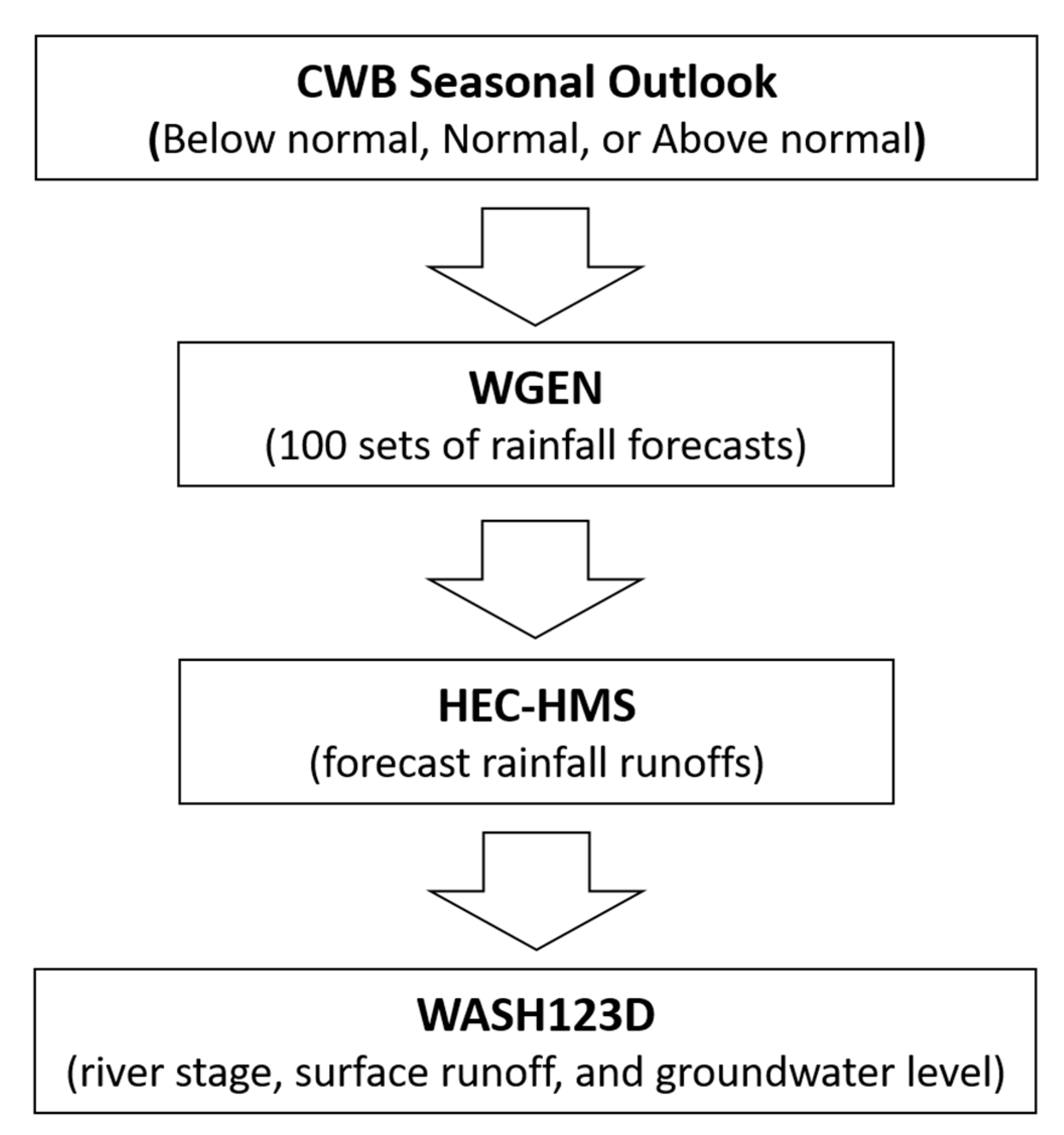
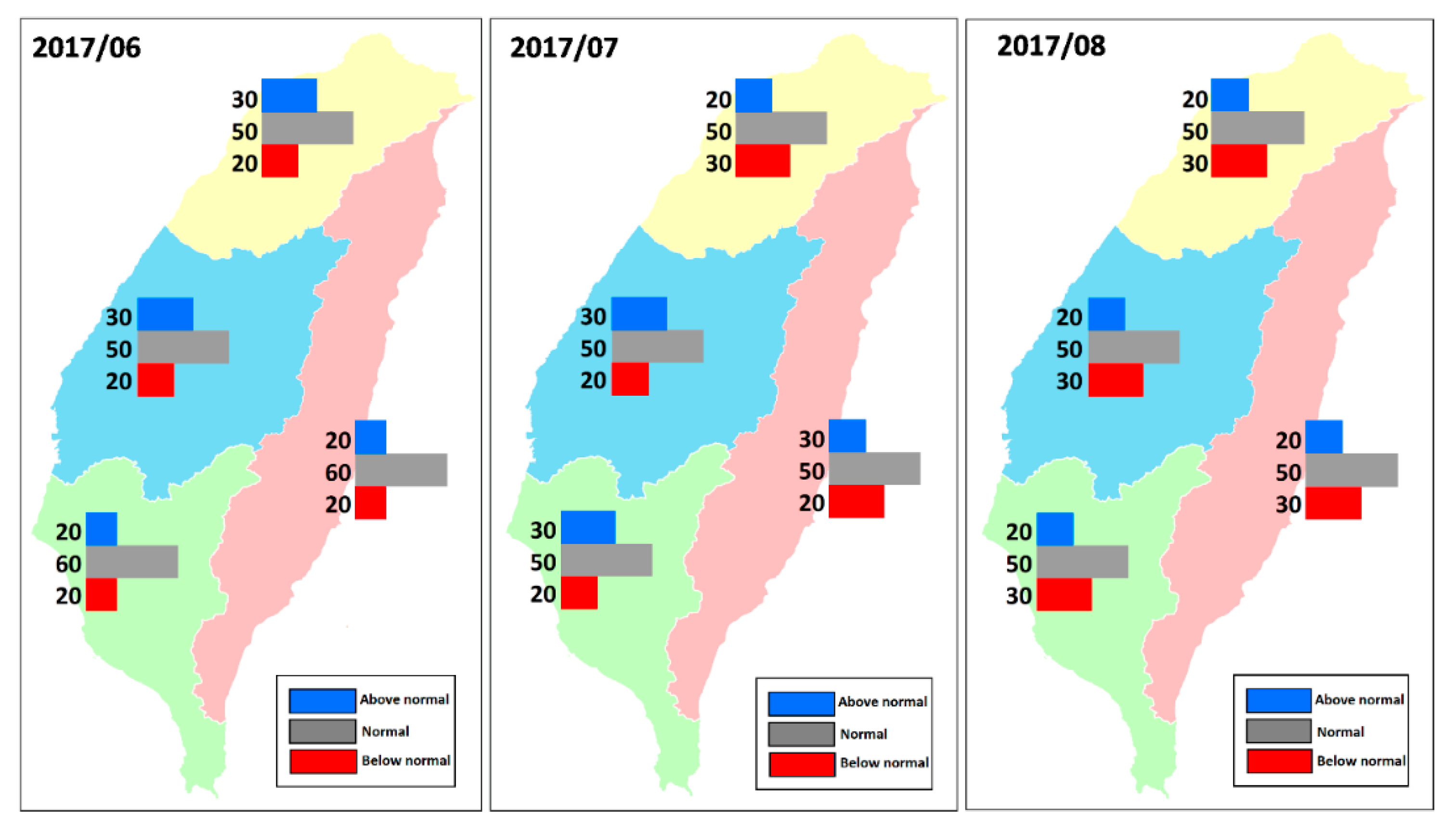
2.1. Seasonal Rainfall Outlook

The Central Weather Bureau (CWB) is responsible for issuing official weather information in Taiwan. The CWB also publicly announces seasonal weather outlooks on the basis of present weather condition, historical statistical records, modeling results (including statistical and numerical weather prediction models), and the subjective judgment of experienced engineers. This study utilized the outcomes of this product to obtain a seasonal perspective (see the first stage in Figure 1). The seasonal weather outlook is the format for prediction of the likelihood of precipitation, as is also the case with many official meteorological service departments and authoritative suppliers of information worldwide, including Japan’s Meteorological Agency, the National Institute of Water and Atmospheric Research in New Zealand, Environment Canada, and the South African Weather Service [32]. Seasonal weather outlooks are usually provided on the CWB website for four regions (i.e., northern, western, southern, and eastern regions) of Taiwan near the end of each month. The probabilities of monthly rainfall, in comparison with historical precipitation data, are issued (“below normal”, “normal”, or “above normal”) for the coming 3 months. These categories are estimated by ranking the observed monthly data, which are obtained from the meteorological station in descending order and divided into three intervals predicting the probability of occurrence. For example, as shown in Figure 2, the probabilities of being “below normal”, “normal”, and “above normal” for the upcoming month of June are 20%, 50%, and 30%, respectively, in the northern region of Taiwan. In other words, there is a 50–50 chance of experiencing a normal amount of rainfall this month.

2.2. Weather Generator (WGEN)

The seasonal weather outlooks from the CWB were coupled with weather generators to produce seasonal rainfall predictions and used as the meteorological inputs for watershed models, as shown in the second stage of Figure 1. The weather generator (WGEN) was based on the model proposed by Tung and Haith [13], used to predict future daily temperature and rainfall. The theory involves either Markov chains or empirical distributions of wet/dry spells [33]. The WGEN requires historical statistical observations records, including the mean, standard deviation, lag 1 serial correlation coefficients, unconditional probability of a rainy day, and the mean precipitation [13]. The WGEN determines daily temperature using the monthly mean and daily records, which follows a first-order Markov chain process [13,17,34]. The daily temperature is expressed as a function of the monthly mean and standard deviation, and a random variable is used to generate an extraordinary occurrence. The Markov chain process, applying historical observations and a random variable between 0 and 1, is examined to identify a rainfall event. In order to generate daily precipitation, two steps are conducted. First, a day is classified as rainy or rainless, and then the amount of rainfall for a rain event is estimated using an exponential distribution. To conduct the prediction, this study used the weather generator, WGEN, supplemented by the rainfall and temperature data recorded from rain gauge stations. Then, on the basis of the long-term seasonal outlook forecast from CWB, the probabilities of monthly rainfall were issued for the upcoming 3 months as the rainfall data. These were taken as inputs for the WGEN to produce 100 sets of rainfall forecasts over the subsequent 3 month simulation. Then, the 25th and 75th percentiles were selected as future rainfall amounts and inputs applied to the hydrological model, WASH123D, for simulating groundwater levels for the next season. The seasonal outlooks in the rainfall forecast of WGEN were derived from CWB, and the historical rainfall observations were obtained from the data of rain gauges.

2.3. Watershed Models

Rainfall-induced surface runoff was obtained from the HEC-HMS model in this study. Three major modules are included in the HEC-HMS: the basin, meteorological, and control specification modules [29,30]. The Soil Conservation Service (SCS) curve number (CN) method is used to calculate the sub-basin loss in the basin module. The parameters of the initial loss, CN value, and impervious percentage are evaluated on the basis of land-use types in the study area. The SCS unit hydrograph method is applied to calculate sub-basin routings, using data from historical records to calculate the discharge and lag time. For the meteorological module, HEC-HMS provides multiple options to generate regional rainfall distribution. The rainfall station weighting method is then used to determine the areal weights for various sub-watersheds using the Thiessen polygon method. Therefore, HEC-HMS was applied to simulate the runoff, and its results were adopted as inputs for subsequent watershed model simulations (see the third stage in Figure 1).

The WASH123D numerical model, developed by Yeh et al. [18,27,28], which conceptualizes the watershed system as a 1D (one-dimensional) stream–river network, 2D (two-dimensional) overland regime, and 3D (three-dimensional) subsurface media, was applied in this study. The model was selected as the most appropriate protocol because it simulates all flows that comprise a watershed. Moreover, it is capable of simulating problems related to various spatial and temporal scales as long as the continuum assumptions are valid. The theory built into WASH123D is based on the conservation laws of fluid and momentum, associated with constitutive relationships among the fluxes, state variables, and appropriately formulated equations for source/sink terms. The governing equations for the one-dimensional river flow are derived from the momentum equation, which is based on the results of the law of conservation of water mass in the continuity equation and linear momentum conservation. For the two-dimensional overland flow, the above assumptions hold except for the conservation principle of linear momentum along with the x-direction and y-direction results in the two momentum equations. The governing equations for subsurface flow through saturated–unsaturated porous media are derived on the basis of the water mass conservation law. The cross-section-averaged 1D diffusive wave equation, depth-averaged 2D diffusive wave equation, and Richard’s 3D equation are applied in the simulations. For surface flow problems, the semi-Lagrangian method (backward particle tracking) is used to solve governing equations. Moreover, the governing equations of subsurface flow are discretized with the Galerkin finite element method [18]. WASH123D has been applied to many regional projects and was chosen by the US Army Corps as the core computational code for coastal and watershed studies [18]. A revamped version of the WASH123D model has been applied to many flood mitigation and groundwater resource problems [7,35,36,37].

3. Study Site and Modeling Configurations

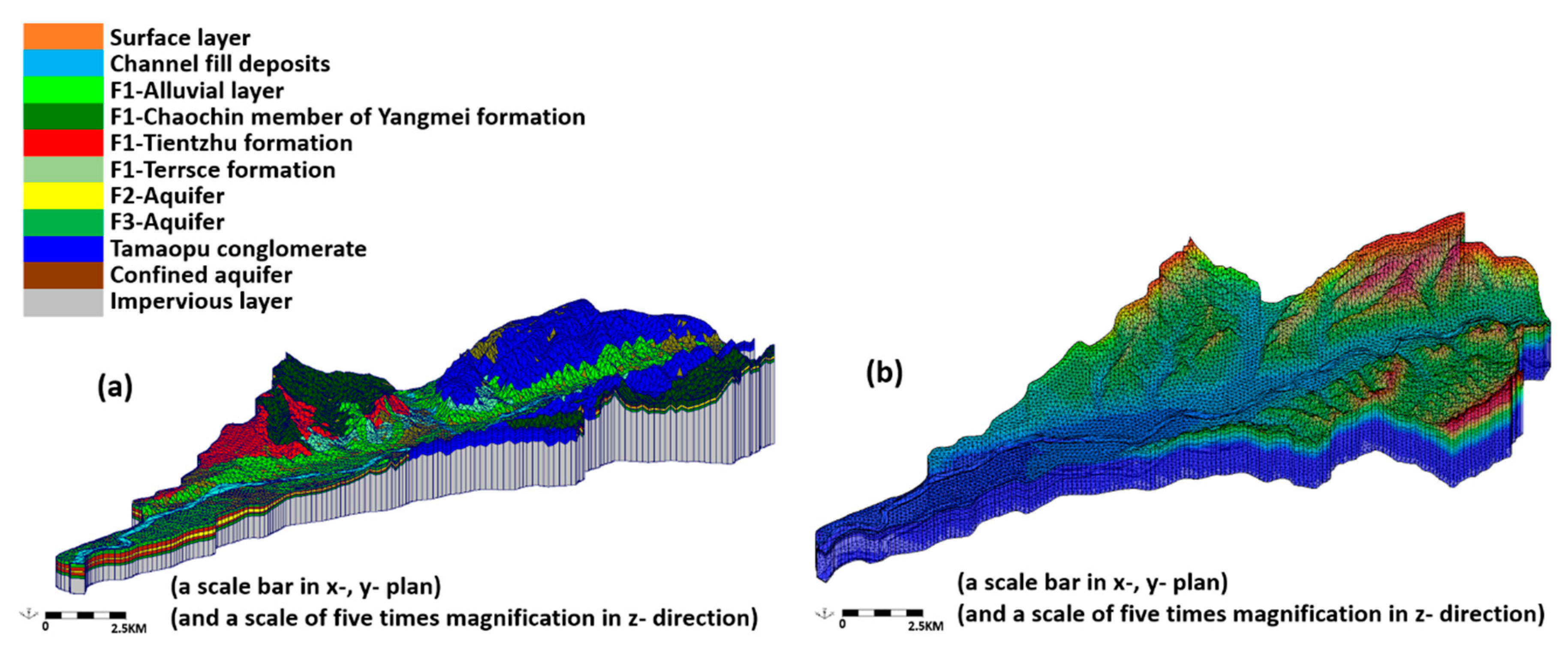
3.1. Basin Information

This study selected the Fengshan Creek basin in northern Taiwan as the study site to test our proposed approach (Figure 3). The Fengshan Creek basin is located in a subtropical zone with parts in the Taoyuan, Hsinchu, and Miaoli areas, where the Hsinchu Science Park is located. Therefore, water resources are particularly crucial because many semiconductor industries are situated in the Hsinchu Science Park. Fengshan Creek originates from Najie Mountain at an altitude of 1320 m. Its trunk stream is approximately 45.45 km long, the longitudinal profile of the river is 1/250, and the catchment area covers 250.1 km². The basin’s meteorological characteristics include 1608 mm of mean annual rainfall and an average of 167 raining days. The rainfall is mainly concentrated in July, August, and September due to typhoons and monsoons. The mean monthly rainfall is 96–270 mm, and the annual rainfall in the area ranges from 1700 to 2700 mm. The maximum monthly rainfall occurred in June 1997. According to the flow gauge records, the annual flow rate ranges from 1.93–17.60 cms (cubic meter per second), with an average of 9.81 cms over 50 years. The maximum flow rate was 3860 cms during Typhoon Toraji in 2001, and the annual runoff from the basin is 376 million m³. The area has a temperate climate, with an average temperature of around 23 °C.

In the simulations, the HEC-HMS hydrological model was applied to generate the discharge rates for the Fengshan Creek basin (zones A and B in Figure 3a), and a physical model, WASH123D, was used for the remaining watershed simulations. As shown in Figure 3b, two rain gauges, one flow gauge, and five hydrogeological drilling wells are located in the Fengshan Creek basin. Measurements were obtained with more than 30 years of records from the Water Resource Agency, Ministry of Economic Affairs, Taiwan (WRA). The land-use types, namely, agricultural (57.3 km²), forestry (133.8 km²), traffic (8.8 km²), water (7.8 km²), buildings (15.9 km²), and other (27.6 km²), were used in this study from field investigations conducted by the National Land Surveying and Mapping Center, Ministry of Interior, Taiwan (NLSC). Hydro-stratigraphic investigations of drilling wells were conducted by the Central Geological Survey (CGS), Ministry of Economic Affairs, Taiwan. The groundwater levels used in this study were from Xinpu well, which is located in the simulated area.

The WASH123D model was applied to simulate surface water and groundwater in the Fengshan Creek basin. The 1D river routing model was constructed using cross-sections taken from field geometry measured by the Second River Management Office, WRA. The setting of 2D surface grids utilizes unstructured meshes, which are constructed using triangular surface elements. The 2D grid is used as the surface layer for the triangular prism meshes for the 3D groundwater modeling. Figure 4a illustrates the hydrogeological classifications of the Fengshan Creek basin. The hydrogeological drilling data from different well sites were applied to build the 3D groundwater layers. As shown in Figure 4a, the upstream part of the Fengshan Creek basin is composed of Tamaopu conglomerate. Part of the upstream and the downstream of the basin is characterized by the Chaochin member of the Yangmei formation, consisting of less permeable sandstone and shale. Other materials (e.g., a general alluvial layer, channel fill deposits, the Tientzhu formation, and Terrsce formation) are also interspersed throughout the watershed. In total, 61,340 grids, 106,371 elements, and nine layers made up the underground grids (Figure 4b).

3.2. Modeling Configuration and Calibrations

Generally, adequate initial conditions of 1D routing are either obtained from measurements or steady-state simulations using the WASH123D model. The 2D ground domain was assumed to be initially dry for all case runs. The well-observed records were interpolated into a 3D domain, and then a steady-state pre-run process was conducted as the initial setup for the subsurface flow simulation. Thus, zero depth and fixed pressure head-dependent boundary conditions were assigned in the 2D and 3D simulations, respectively. Simulations for the years 2013–2015 were conducted to determine the appropriate parameters for the hydrological models and evaluate the model performance. Then, the initial loss, lag time, CN values, and Manning’s coefficients of the 1D stream–river network and 2D overland regime were determined. The hydraulic conductivity was determined on the basis of the long-term period for the groundwater simulation. The modeling parameters and simulation errors are listed in

Table 1. Parameters used in the Soil Conservation Service (SCS) curve method and WASH123D of Fengshan Creek basin (extracted from Wu and Shih [7]). CN, curve number.

HEC-HMS	WASH123D
SCS curve	Channels (1D) Mn	Surface land (2D) Mn	Groundwater layers (3D) Ks (m/s)
Initial loss (4.0 mm) Non-infiltration covers (17.6–22.1%) Lag time (131.2–147.2 min.) CN (51.9–62.3)	0.036–0.029	Metropolitan (0.120) Non-metropolitan (0.280) Other (0.085)	Gravel (1 × 10−3) Mud or fine silt (4 × 10−6) River sediment (2 × 10−5) Aquifers (1 × 10−3 to 1 × 10−5) Impermeable layer (1 × 10−8)

and

Table 2. Error indicators for evaluating the performance of the surface water/groundwater model.

Model	Events	Coefficient of Determination (R2)	Root-Mean-Square Error (RMSE)	Nash–Sutcliffe Model Efficiency Coefficient (CE)
Surface water	Soulik (2013)	0.910	0.253	0.896
	Kong-rey (2013)	0.832	0.209	0.791
	Soudelor (2015)	0.817	0.479	0.803
	Rainfall event (2015)	0.840	0.176	0.807
	Average	0.850	0.279	0.824
Groundwater	2013 (1 January–31 December)	0.475	0.363	0.459
	2014 (1 January–31 March)	0.763	0.108	0.670
	2014 (1 July–31 October)	0.638	0.195	0.471
	2015 (1 April–31 October)	0.550	0.460	0.885
	Average	0.607	0.282	0.621

. Wu and Shih [7] confirmed the good agreement between the simulation and observations results for both surface water and groundwater tables, in which error indicators of R², root-mean-square error (RMSE), and efficiency coefficient (CE) were 0.850, 0.279m, and 0.824, respectively, for the river stage and 0.607, 0.281, and 0.621 for the groundwater table. Therefore, the simulations adopted the setups by the above research to further improve the feasibility of this study.

The flow patterns of the rainfall-induced stream hydrograph and groundwater table were quite different, as presented in Figure 5, which illustrates the simulated hydrographs of both surface water and groundwater from 4 July to 17 July in 2013 and 12 May to 27 May in 2015. These two periods, 2013 and 2015, were selected due to the insufficient rainfall data in 2014. In Figure 5, it can be seen that the river stage corresponded quite well to the rainfall intensity. The time lag was almost 1 h between the maximum rainfall intensity and peak flow. This response is typical for watersheds of Taiwan, which are characterized by rugged and steep topography. Thus, it is difficult to capture and store surface water for human consumption. However, the groundwater level has a different pattern with a relatively mild fluctuation in comparison to the river stages. The studies found there was a 2 day average lag (approximately 45 to 52 h) for the groundwater to reach the peak level after the occurrence of extreme rainfall. Therefore, the exact evaluation of the groundwater level can contribute to the effective utilization of water resources in Taiwan.

4. Results and Discussion

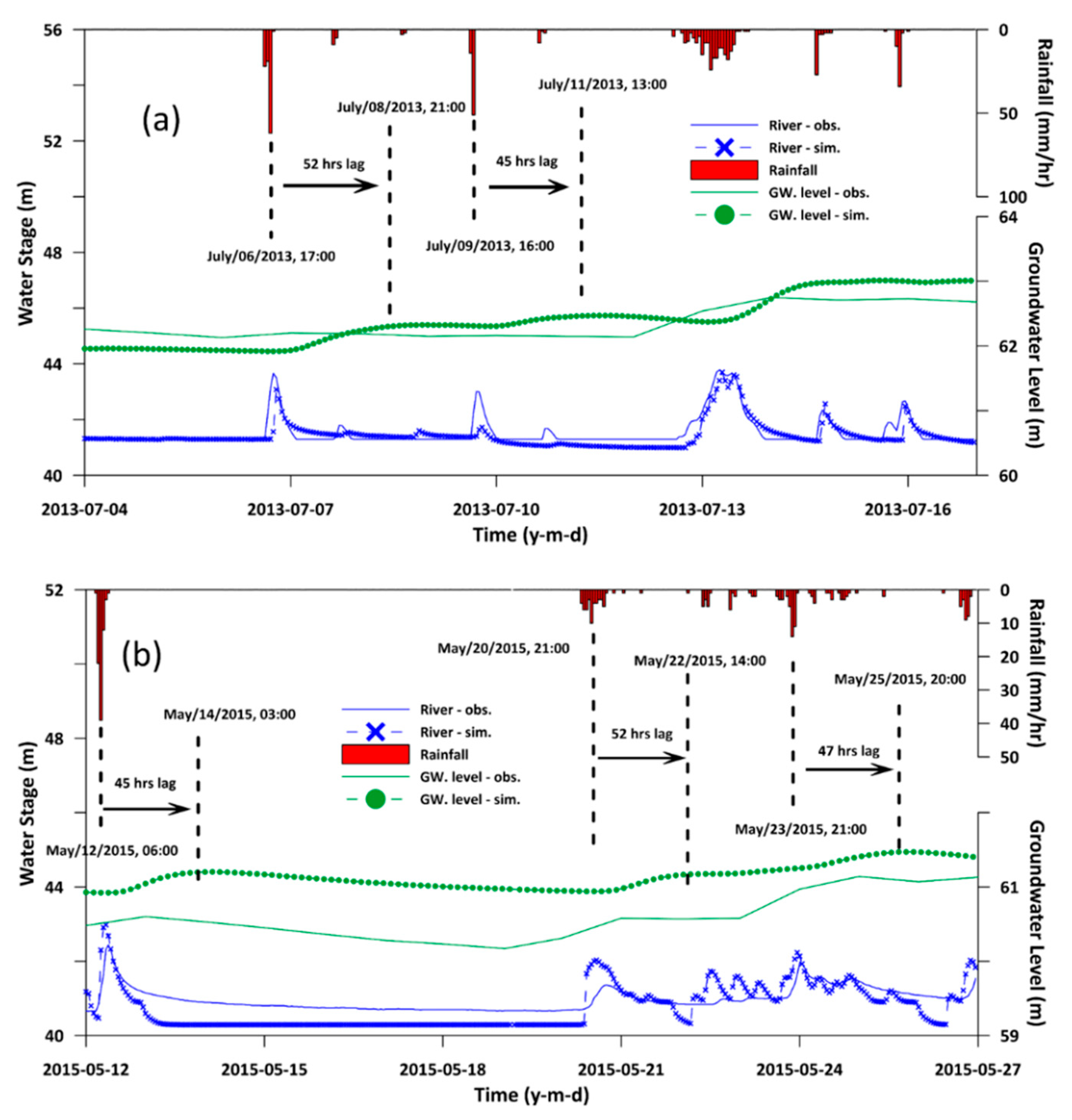
4.1. Model Validation

Simulation settings for all parameters in the modeling calibration were fixed. To validate the parameters used in the model, a full-year simulation of 2017 was conducted. As shown in Figure 6a, a comparison of groundwater table variation between simulation and observation data was conducted. This shows that the groundwater level hydrograph of simulation agreed with that of observations at Xinpu station, and the general trends were also comparable before 18 August 2017. The results prior to 18 August show that the errors between simulated and observed groundwater levels were R² of 0.801 and RMSE of 0.228 m; thus, the simulation model yielded a great result. However, following 18 August 2017, there was a sudden decline in groundwater level observations, resulting in a discrepancy between simulated and observed groundwater level. The error indicators of the simulation without considering pumping after 18 August 2017, shown as cross dots, were R² of 0.052 and RMSE of 0.862 m. In fact, errors gradually increased after this. Anthropogenic pumping activities were expected to be the primary reason. A crucial discharge mechanism or substantial water use could have caused this abnormal drawdown, which is not easily incorporated into the simulation. As the rainfall during this period was not sufficient to replenish the groundwater, and the amount of groundwater pumped increased, a drawdown in the water level inevitably occurred. Therefore, the effect of pumping was further considered and taken as a factor in the following simulation. Note that records of pumping rate were only adopted from the registered well, while the records from the unregistered well were not exploited in this study because the amount of pumping water from the unregistered well is unknown. Moreover, it was considered minor due to our study site not belonging to the land subsidence areas in Taiwan. Thus, there was not a problem of groundwater being over-pumped. Moreover, cases of pumping groundwater were found to be rare after conducting an investigation of unregistered wells and giving well permits in recent years. Thus, the effect of unregistered well pumping is relatively minor. The pumping rate of the registered well at Xinpu Station was added to the simulation with 3000 cmd (cubic meter per day, cmd). The results are shown in Figure 6a. The hydrograph revealed that the simulated groundwater level when considering pumping, shown as green dots, corresponded with the observed hydrograph (R² of 0.256, RMSE of 0.749 m). The simulation result was clear as the error of RMSE was minimized, and the value of R² increased after the effect of pumping was adopted in the study. The simulation result was improved by including anthropogenic pumping. Moreover, this also implies that these parameters are suitable for simulating groundwater in the Fengshan Creek basin.

In Figure 6b, there was an extreme event showing the flow patterns for both river and groundwater from 2 June to 14 June in 2017. The simulation results reveal that the simulated hydrograph of the river stage and groundwater level corresponded with the observation results in both the raising and recession periods for the water stage and groundwater level. The lag time following a rainfall event was approximately 2 days (51 h), which is consistent with the average lag time of 2013–2015 simulations. The errors between simulated and observed river water levels were R² of 0.729 and RMSE of 0.418 m, while the errors between simulated and observed groundwater levels were R² of 0.826 and RMSE of 0.426 m. According to the above data (surficial: R² of 0.729 and RMSE of 0.418 m; groundwater: R² of 0.826 and RMSE of 0.426 m), the high correlation between simulated and observed water level, whether stream flow or groundwater, suggests that the rise of surficial rainfall-induced groundwater level can be accurately assessed by our simulation. In short, the simulation model demonstrated both stability and feasibility as its results agreed with the observed groundwater table. The validation results confirmed that these parameters are practical and adequate for subsequent seasonal assessment.

4.2. Rainfall Generation by WGEN

Rainfall records from the Guanxi and Xinpu gauges were taken as inputs for the WGEN to produce 100 sets of rainfall forecasts over the subsequent 3 months of simulation according to the CWB’s classification criteria of precipitation forecast probabilities: “below normal”, “normal”, or “above normal”. A single precipitation forecast to assess groundwater level might produce an unreliable result and a huge discrepancy because of its predicting uncertainty. Thus, in order to minimize the error, the strategy involving 25th to 75th percentiles of simulated precipitation was used for the simulation of groundwater table.

Table 3. Ten sets of seasonal rainfall outlooks and real rainfall occurrences of Guanxi station in 2018.

Guanxi Station	2018	Real Occurrence (mm)	25th Percentile of Simulation Rainfall (mm)	75th Percentile of Simulation Rainfall (mm)	Seasonal Forecast A/N/B	Hit/Miss
1st	Jan.	267.0	55.2	55.5	10/60/30
	Feb.	147.5	101.0	154.9	10/60/30
	Mar.	57.0	121.6	267.3	10/60/30
Total		471.5	277.8	477.7		Hit
2nd	Feb.	147.5	19.2	146.3	10/50/40
	Mar.	57.0	232.0	237.7	20/60/20
	Apr.	85.5	111.0	279.2	30/50/20
Total		290.0	362.2	663.2		Miss
3rd	Mar.	57.0	120.0	353.9	20/60/20
	Apr.	85.5	107.9	122.1	30/50/20
	May	85.0	211.3	277.9	30/50/20
Total		227.5	439.2	753.9		Miss
4th	Apr.	85.5	233.7	326.2	20/50/30
	May	85.0	227.5	374.0	20/50/30
	Jun.	177.0	232.6	274.6	30/50/20
Total		347.5	693.8	974.8		Miss
5th	May	85.0	240.2	355.5	10/50/40
	Jun.	177.0	346.0	396.5	20/50/30
	Jul.	199.0	231.3	603.8	20/50/30
Total		461.0	817.5	1328.8		Miss
6th	Jun.	177.0	387.6	580.6	20/50/30
	Jul.	199.0	147.2	194.8	20/50/30
	Aug.	659.5	139.8	274.5	20/50/30
Total		1035.5	674.6	1049.9		Hit
7th	Jul.	199.0	190.3	249.3	30/50/20
	Aug.	659.5	177.7	235.0	20/50/30
	Sep.	182.0	296.0	335.8	20/50/30
Total		1040.5	664	820.1		Miss
8th	Aug.	659.5	315.9	377.9	20/50/30
	Sep.	182.0	117.1	361.4	20/50/30
	Oct.	84.5	45.3	52.6	20/50/30
Total		926.0	478.3	791.9		Miss
9th	Sep.	182.0	224.6	442.8	20/50/30
	Oct.	84.5	55.4	114.8	10/60/30
	Nov.	47.5	64.7	65.9	20/50/30
Total		314.0	344.7	623.5		Miss
10th	Oct.	84.5	57.9	229.1	10/60/30
	Nov.	47.5	8.7	29.5	10/50/40
	Dec.	39.0	67.2	138.2	20/60/20
Total		171.0	133.8	376.0		Hit

Note: N, normal; B, below normal; A, above normal.

and

Table 4. Ten sets of seasonal rainfall outlooks and real rainfall occurrences of Xinpu station in 2018.

Xinpu Station	2018	Real Occurrence (mm)	25th Percentile of Simulation Rainfall (mm)	75th Percentile of Simulation Rainfall (mm)	Seasonal Forecast A/N/B	Hit/Miss
1st	Jan.	272.0	31.0	83.2	10/60/30
	Feb.	98.5	99.9	218.8	10/60/30
	Mar.	54.0	119.9	166.4	10/60/30
Total		424.5	250.8	468.4		Hit
2nd	Feb.	98.5	78.9	180.7	10/50/40
	Mar.	54.0	93.0	235.7	20/60/20
	Apr.	54.0	161.2	217.7	30/50/20
Total		206.5	333.1	634.1		Miss
3rd	Mar.	54.0	104.0	139.8	20/60/20
	Apr.	54.0	129.3	238.1	30/50/20
	May	49.0	195.3	313.1	30/50/20
Total		157.0	428.6	691		Miss
4th	Apr.	54.0	87.7	108.1	20/50/30
	May	49.0	209.7	355.3	20/50/30
	Jun.	113.0	325.7	335.4	30/50/20
Total		216.0	623.1	798.8		Miss
5th	May	49.0	262.1	346.0	10/50/40
	Jun.	113.0	147.3	180.3	20/50/30
	Jul.	69.0	135.7	156.3	20/50/30
Total		231.0	545.1	682.6		Miss
6th	Jun.	113.0	123.1	234.5	20/50/30
	Jul.	69.0	58.9	138.6	20/50/30
	Aug.	251.0	240.2	280.2	20/50/30
Total		433.0	422.2	653.3		Hit
7th	Jul.	69.0	116.7	147.1	30/50/20
	Aug.	251.0	157.0	176.5	20/50/30
	Sep.	202.5	111.9	220.4	20/50/30
Total		522.5	385.6	544		Hit
8th	Aug.	251.0	144.8	212.6	20/50/30
	Sep.	202.5	113.7	134.1	20/50/30
	Oct.	54.0	64.3	115.9	20/50/30
Total		507.5	322.8	462.6		Miss
9th	Sep.	202.5	103. 7	197.0	20/50/30
	Oct.	54.0	79.4	99.2	10/60/30
	Nov.	42.0	23.0	50.2	20/50/30
Total		298.5	206.1	346.4		Hit
10th	Oct.	54.0	62.5	75.8	10/60/30
	Nov.	42.0	37.4	62.5	10/50/40
	Dec.	36.0	40.9	64.3	20/60/20
Total		132.0	140.8	202.6		Miss

Note: N, normal; B, below normal; A, above normal.

show the results of the seasonal rainfall forecast issued by the CWB in 2018. The monthly rainfall forecasts for the 100 sets of simulated data issued by WGEN were arranged in ascending order. Then, the 25th and 75th percentiles in ascending order were selected as future rainfall amounts and inputs applied to the hydrological models for simulating groundwater levels for the next season. As shown in Table 3 and Table 4, the seasonal rainfall outlook announced by the CWB was mostly predicted as “normal” rainfall in 2018. To assess the performance of the seasonal rainfall forecasts, these two tables compare the 3 month rainfall predictions and the real rainfall recorded at the Guanxi and Xinpu rainfall gauges. For the Guanxi station, the 25th and 75th percentiles of simulated rainfall were 277.8 mm and 477.7 mm, respectively, from January to March, as the first seasonal rainfall outlook. However, the amount of real rainfall in the same period was 471.5 mm, which shows that the simulation corresponded with the actual situation. The same situation was found in the sixth and tenth seasonal rainfall outlooks from June to August and October to December in 2018. On the other hand, the amount of seasonal rainfall in the second to fifth and ninth outlooks overestimated the real rainfall. In the seventh and eighth seasonal rainfall outlooks, the amount of real rainfall was underestimated. For the Xinpu station, the results indicate that the seasonal outlook in the first, sixth, seventh, and ninth outlooks successfully forecasted the real rainfall. The real rainfall in the second to fifth and tenth outlooks was overestimated. The eighth seasonal rainfall outlook underestimated the real rainfall.

This study used the seasonal forecast from CWB to calculate the 25th to 75th percentiles of simulated precipitation from WGEN. A comparison between this simulated precipitation and the actual precipitation was made to study the hitting rate. Thus, actual precipitation within the simulated precipitation (25th–75th) can represent an accurate prediction. Then, we added up the monthly precipitation to examine whether the annual precipitation at Guanxi and Xinpu station was within the simulated precipitation in terms of 25th to 75th percentiles. According to the above results, the annual values of the 25th and 75th percentiles of simulated rainfall were within 1921–3285 mm at the Guanxi station. The amount of real rainfall was 2031 mm. This shows that its seasonal rainfall outlook was around 30% accurate for the 3 month forecast, but the total amount of annual rainfall was within the range of 25th and 75th percentiles (1921–3285 mm). Similarly, at the Xinpu station, its seasonal rainfall outlook was about 40% accurate in terms of hitting rate, but the amount of annual rainfall (1295 mm) was within the range of 25th and 75th percentiles (1193–1852 mm). In addition, according to the result of Table 3 and Table 4, the results of seasonal outlook overestimated the rainfall from February to May but not January in both of these gauges. The overestimation presented in the amount of actual rainfall was less than that of the 25th percentile of WGEN rainfall productions. This shows that the seasonal rainfall outlook easily overestimated the real rainfall during the dry season (November to April in Taiwan). Note that the amount of annual rainfall was within the range of 25th and 75th percentiles, although there were some missed seasonal forecasts as mentioned above.

4.3. Groundwater Table According to Seasonal Rainfall Outlooks

Figure 7 illustrates all 3 month groundwater outlooks at the Xinpu well station from January to October in 2018. The simulation parameters were adopted on the basis of the above validation results. Furthermore, in this study, only monthly pumping data were available. Thus, 3000 cmd of pumping rate for the registered well at Xinpu Station was used for our simulation. In Figure 7, the blue dots represent the results of groundwater level simulation according to the rainfall observation from gauges. The red rectangles and green triangles of Figure 7 are the results of groundwater level simulation as the 25th and 75th percentiles from seasonal rainfall forecasts, respectively. The simulation results using observation data demonstrate that they corresponded with the groundwater measurement. In other words, the parameters used in the study used were adequate, as they could reasonably reflect the variation of the groundwater table.

In Table 3 and Table 4, the total forecast rainfall in terms of the 25th to 75th percentiles ranged from 331.0 to 423.0 mm for the first seasonal rainfall outlook from January to March at the Guanxi station. The real rainfall occurrence (471.5 mm) was within the forecast interval (277.8 mm and 477.7 mm). A similar situation occurred for the 3 month rainfall outlook from January to March at the Xinpu station. The value of simulated groundwater levels fit the observation values quite well from January to March in 2018, as shown in Figure 7a. Since the precipitation forecasts overestimated the real rainfall occurrence for the second to fifth seasonal rainfall outlooks from February–April to May–July, the groundwater levels during these periods were also overestimated, as indicated in Figure 7b–e. Regardless of the underestimation of rainfall at the Guanxi station and the overestimation of rainfall at the Xinpu station in the sixth seasonal rainfall outlook, the simulation revealed a comparable result to the observation from June to August in 2018. In fact, the above results are also presented in Figure 7f–h. The result of the groundwater simulation, which took the rainfall from the gauges as the inputs, corresponded with the observation result, showing the applicability of this simulation. However, even though the rainfall amounts for both stations were underestimated, such as in Figure 7g,h, the overall simulations of groundwater table corresponded to the observation result because of the high rainfall during this period where the observation water table was 60.333 m; the simulation result was 60.513 m and the 25th–75th percentiles of the simulated rainfall-induced water table were 60.465 m–60.814 m, as shown in Figure 7g. In Figure 7h, the observation rainfall-induced groundwater level was 59.788 m, while the simulation result was 59.859 m and the 25th–75th percentiles of simulated rainfall were 60.365 m–60.518 m. Therefore, the groundwater generated by seasonal forecast was comparable to the real groundwater table during the raining season. As shown in Figure 7i,j, the result of groundwater table according to the seasonal forecast was higher than the observation result. This was caused by the overestimation of these two gauges, which resulted in a high groundwater level.

The above results show insufficient rainfall during the spring and Mei-yu season of 2018. Mei-yu is a weather and climate phenomenon in subtropical Asia. It is caused by the Mei-yu front and continuous rainfall for nearly 2 months during late spring and early summer in Taiwan (May and June). In fact, on average, the historical spring rainfall values from February to April and Mei-yu rainfall from May to June are approximately 527.0 mm and 559.0 mm, respectively, for our study site. However, the amounts of spring rainfall at the Guanxi and Xinpu stations were 290.0 mm and 206.0 mm, respectively, in 2018, which were much lower than the average. In addition, the amounts of Mei-yu rainfall were 262.0 mm and 162.0 mm for the Guanxi and Xinpu stations, respectively, which were also much lower than the average. According to the above results, the forecasted groundwater level was overestimated before the high-water-level period, as shown in Figure 7a–e. Then, when the typhoon season started, the total annual rainfall amounts in 2018 at the Guanxi and Xinpu stations were 2031 and 1295 mm, respectively. In 2018, the amount of rainfall from July to September at the Guanxi station was approximately 1040 mm, which was more than half of the total annual rainfall amount. At the Xinpu station, the rainfall amount from July to September in year 2018 was approximately 522 mm, which was near the average of historical records. However, with the lower accuracy of rainfall forecast after October, the lack of precipitation was the reason for the decreasing groundwater levels from September to December, as shown in Figure 7i,j.

It can be seen that the predicted rainfall is indeed the crucial factor affecting simulated groundwater levels. When rainfall predictions agreed with rain gauge observation, the hydrograph patterns in the groundwater simulations were similar to the measurement of seasonal groundwater outlooks. In the 2018 seasonal forecast, the groundwater level was overestimated because the amount of monthly rainfall was far lower than the average of the historical record in some dry season months, as shown in Figure 7c–j. However, the amount of rainfall returned to normal values during the wet seasons, which contributed to the agreement between the seasonal forecast and observation, as shown in Figure 7f–h. It can be clearly seen that the precipitation overestimation of seasonal forecasting during the dry seasons was the major cause for the above conditions. Although assessing groundwater level with a unified seasonal outlook and hydrological modelling projection is feasible, it should be noted that the phenomenon of groundwater level tends to be overestimated during the dry season. In cases of a low groundwater table, unregistered extraction by private wells is an issue that must be considered, as this might affect the accuracy of the results. In fact, most industrial users need to register for water use in Taiwan. Unregistered water use, mainly for agricultural or aqua-culture purposes, can result in over-extraction from wells during the dry periods. This is also a major cause of land subsidence along the southwest coast of Taiwan. Over-extraction coupled with unregistered water use can cause significant discrepancies when the groundwater level is low during dry seasons. In fact, in terms of consequentialism, the simulation result for 2018 in this study was not quite adequate enough. However, this established approach may be improved in the future through many other experiments. These may involve addressing the acceptable error range for our approach, e.g., by widening the range of 25th–75th percentiles, utilizing safety factors, and conducting groundwater level management.

5. Conclusions

This study indicated that groundwater level assessment is achievable by combining the seasonal rainfall outlook approach and hydrological model simulations. The model calibration revealed that both hydrographic and error indicators verified its good performance. The validation results confirmed that these parameters are practical for subsequent seasonal assessments and appropriate for in situ conditions. Thus, this study demonstrated a stable and good performance of the modeling results. It also indicated that the groundwater level can be accurately obtained as long as the rainfall inputs are accurate. Thus, the method proposed by this study was confirmed to be feasible. For example, the rainfall results yielded by WGEN in terms of the 25th and 75th percentiles of simulated rainfall of 2018 were within 2149 and 3056 mm at the Guanxi station and within 1227 and 1714 mm at the Xinpu station. The annual rainfall at the Guanxi station (2031 mm) hit the interval (1921–3285 mm), while that at the Xinpu station (1295 mm) was within the range of the 25th and 75th percentiles (1193–1852 mm), even though the accuracy rate for the 3 month seasonal forecast had slight errors. However, the discrepancies in terms of groundwater table were more extensive in the dry season than in the rainy season. The groundwater simulations revealed overestimated results because the amount of monthly rainfall was far lower than the average of the historical record in some dry season months. However, the amount of rainfall returned to normal during the wet seasons, which provided results corresponding with seasonal forecasts and observations. These discrepancies might have been due to anthropogenic activities, such as unregistered pumping. Overcoming this in future work will require more measurement data.

References

1. Aeschbach-Hertig, W.; Gleeson, T. Regional strategies for the accelerating global problem of groundwater depletion. Nat. Geosci. 2012, 5, 853. [Google Scholar] [CrossRef]
2. Oki, T.; Kanae, S. Global hydrological cycles and world water resources. Science 2006, 313, 1068–1072. [Google Scholar] [CrossRef] [PubMed] [Green Version]
3. Mackay, J.; Jackson, C.; Brookshaw, A.; Scaife, A.; Cook, J.; Ward, R. Seasonal forecasting of groundwater levels in principal aquifers of the United Kingdom. J. Hydrol. 2015, 530, 815–828. [Google Scholar] [CrossRef] [Green Version]
4. Prudhomme, C.; Hannaford, J.; Harrigan, S.; Boorman, D.; Knight, J.; Bell, V.; Jackson, C.; Svensson, C.; Parry, S.; Bachiller-Jareno, N.; et al. Hydrological Outlook UK: Operational streamflow and groundwater level forecasting system at monthly to seasonal time scales. Hydrol. Sci. J. 2017, 62, 2753–2768. [Google Scholar] [CrossRef] [Green Version]
5. Emerton, R.; Zsoter, E.; Arnal, L.; Cloke, H.L.; Muraro, D.; Prudhomme, D.; Stephens, E.M.; Salamon, P. Developing a global operational seasonal hydro-meteorological forecasting system: GloFAS-Seasonal v1.0. Geosci. Model Dev. 2018, 11, 3327–3346. [Google Scholar] [CrossRef] [Green Version]
6. Hsu, H.H.; Chen, C.T.; Lu, M.M.; Chen, Y.M.; Chou, C.; Wu, Y.C. Climate Change in Taiwan: Scientific Report 2011; National Science and Technology Center for Disaster Reduction: New Taipei City, Taiwan, 2011; p. 67. (In Chinese)
7. Wu, R.S.; Shih, D.S. Modeling hydrological impacts of groundwater level in the context of climate and land cover change. Terr. Atmos. Ocean. Sci. 2018, 29, 341–353. [Google Scholar] [CrossRef] [Green Version]
8. Clark, M.P.; Hay, L.E. Use of medium-range numerical weather prediction model output to produce forecasts of streamflow. J. Hydrometeorol. 2004, 5, 15–32. [Google Scholar] [CrossRef]
9. Wood, A.W.; Maurer, E.P.; Kumar, A.; Lettenmaier, D.P. Long-range experimental hydrologic forecasting for the eastern United States. J. Geophys. Res. Atmos. 2002, 107, ACL 6-1–ACL 6-15. [Google Scholar] [CrossRef]
10. Bastola, S.; Misra, V.; Li, H. Seasonal hydrological forecasts for watersheds over the southeastern United States for the boreal summer and fall seasons. Earth Interact 2013, 17, 1–22. [Google Scholar] [CrossRef]
11. Verdin, A.; Rajagopalan, B.; Kleiber, W.; Podestá, G.; Bert, F. A conditional stochastic weather generator for seasonal to multi-decadal simulations. J. Hydrol. 2018, 556, 835–846. [Google Scholar] [CrossRef]
12. Richardson, C.W. Stochastic simulation of daily precipitation, temperature, and solar radiation. Water Resour. Res. 1981, 17, 182–190. [Google Scholar] [CrossRef]
13. Tung, C.P.; Liu, T.M.; Chen, S.W.; Ke, K.Y.; Li, M.H. Carrying capacity and sustainability appraisals on regional water supply systems under climate change. Int. J. Environ. Clim. Chang. 2014, 4, 27–44. [Google Scholar] [CrossRef]
14. Pickering, N.B.; Stedinger, J.R.; Haith, D.A. Weather input for nonpoint-source pollution models. J. Irrig. Drain. Eng. 1988, 114, 674–690. [Google Scholar] [CrossRef]
15. Selker, J.S.; Haith, D.A. Development and Testing of Single-Parameter Precipitation Distributions. Water Resour. Res. 1990, 26, 2733–2740. [Google Scholar] [CrossRef] [Green Version]
16. Liu, T.M.; Tung, C.P.; Ke, K.Y.; Chuang, L.H.; Lin, C.Y. Application and development of a decision-support system for assessing water shortage and allocation with climate change. Paddy Water Environ. 2009, 7, 301–311. [Google Scholar] [CrossRef]
17. Tung, C.P.; Haith, D.A. Global-warming effects on New York stream flows. J. Water Resour. Plan. Manag. 1995, 121, 216–225. [Google Scholar] [CrossRef]
18. Yeh, G.T.; Shih, D.S.; Cheng, J.R.C. An integrated media, integrated processes watershed model. Comput. Fluids 2011, 45, 2–13. [Google Scholar] [CrossRef]
19. Harbaugh, A.W. MODFLOW-2005, the US Geological Survey modular ground-water model—The ground-water flow process. In Techniques and Methods 6-A16; U.S. Geological Survey: Reston, VA, USA, 2005. [Google Scholar]
20. Markstrom, S.L.; Niswonger, R.G.; Regan, R.S.; Prudic, D.E.; Barlow, P.M. GSFLOW-Coupled Ground-water and Surface-water FLOW model based on the integration of the Precipitation-Runoff Modeling System (PRMS) and the Modular Ground-Water Flow Model (MODFLOW-2005). In Techniques and Methods 6-D1; U.S. Geological Survey: Reston, VA, USA, 2008; 240p. [Google Scholar]
21. Kim, N.W.; Chung, I.M.; Won, Y.S.; Arnold, J.G. Development and application of the integrated SWAT–MODFLOW model. J. Hydrol. 2008, 356, 1–16. [Google Scholar] [CrossRef]
22. Bailey, R.T.; Wible, T.C.; Arabi, M.; Records, R.M.; Ditty, J. Assessing regional-scale Spatio-temporal patterns of groundwater-surface water interactions using a coupled SWAT-MODFLOW model. Hydrol. Process. 2016, 30, 4420–4433. [Google Scholar] [CrossRef]
23. Bailey, R.; Rathjens, H.; Bieger, K.; Chaubey, I.; Arnold, J. SWATMOD-Prep: Graphical user interface for preparing coupled SWAT-MODFLOW simulations. J. Am. Water Resour. Assoc. 2017, 53, 400–410. [Google Scholar] [CrossRef]
24. Ross, M.; Geurink, J.; Said, A.; Aly, A.; Tara, P. Evapotranspiration conceptualization in the HSPF-MODFLOW integrated models. J. Am. Water Resour. Assoc. 2005, 41, 1013–1025. [Google Scholar] [CrossRef]
25. Swain, E.D. Implementation and Use of Direct-Flow Connections in a Coupled Ground-Water and Surface-Water Model. Groundwater 1994, 32, 139–144. [Google Scholar] [CrossRef]
26. Refsgaard, J.C.; Storm, B. MIKE SHE, in Computer Models of Watershed Hydrology; Singh, V.P., Ed.; Water Resources Publications: Littleton, CO, USA, 1995; pp. 809–846. [Google Scholar]
27. Yeh, G.T.; Cheng, H.P.; Cheng, J.R.; Lin, J.H. A numerical model to simulate water flow and contaminant and sediment transport in watershed systems of 1-D stream-river network, 2-D overland regime, and 3-D subsurface media (WASH123D: Version 1.0). In Technical Report CHL-98-19; Waterways experiment station, US Army Corps of Engineers: Vicksburg, MS, USA, 1998. [Google Scholar]
28. Yeh, G.T.; Huang, G.; Zhang, F.; Cheng, H.P.; Lin, H.C. WASH123D: A Numerical Model of Flow, Thermal Transport, and Salinity, Sediment, and Water Quality Transport in WAterSHed Systems of 1-D Stream-River Network, 2-D Overland Regime, and 3-D Subsurface Media; Office of Research and Development: Orlando, FL, USA, 2005. [Google Scholar]
29. US Army Corps of Engineers (USACE). Hydrologic Modeling System HEC-HMS: Technical Reference Manual; Hydrologic Engineering Center: Davis, CA, USA, 2000. [Google Scholar]
30. US Army Corps of Engineers (USACE). Hydrologic Modeling System HEC-HMS: Applications Guide; Hydrologic Engineering Center: Davis, CA, USA, 2008. [Google Scholar]
31. Halwatura, D.; Najim, M. Application of the HEC-HMS model for runoff simulation in a tropical catchment. Environ. Model Softw. 2013, 46, 155–162. [Google Scholar] [CrossRef]
32. Yu, P.S.; Yang, T.C.; Kuo, C.M.; Wang, Y.T. A stochastic approach for seasonal water-shortage probability forecasting based on seasonal weather outlook. Water Resour. Manag. 2014, 28, 3905–3920. [Google Scholar] [CrossRef]
33. Semenov, M.A.; Brooks, R.J. Spatial interpolation of the LARS-WG stochastic weather generator in Great Britain. Clim. Res. 1999, 11, 137–148. [Google Scholar] [CrossRef] [Green Version]
34. Wu, R.S.; Haith, D.A. Land use, climate, and water supply. J. Water Resour. Plan. Manag. 1993, 119, 685–704. [Google Scholar] [CrossRef]
35. Shih, D.S.; Yeh, G.T. Identified model parameterization, calibration, and validation of the physically distributed hydrological model WASH123D in Taiwan. J. Hydrol. Eng. 2011, 16, 126–136. [Google Scholar] [CrossRef]
36. Shih, D.S.; Liau, J.M.; Yeh, G.T. Model Assessments of Precipitation with a Unified Regional Circulation Rainfall and Hydrological Watershed Model. J. Hydrol. Eng. 2012, 17, 43–54. [Google Scholar] [CrossRef]
37. Shih, D.S.; Hsu, T.W.; Chang, K.C.; Juan, H.L. Implementing Coastal Inundation Data with an Integrated Wind Wave Model and Hydrological Watershed Simulations. Terr. Atmos. Ocean Sci. 2012, 23, 513–525. [Google Scholar] [CrossRef] [Green Version]
Figure 1. Flowchart of the proposed method. CWB, Central Weather Bureau of Taiwan; WGEN, weather generator; HEC-HMS, hydrologic modeling system; WASH123D, watershed systems of one-dimensional (1D) stream–river network, 2D overland regime, and 3D subsurface media.
Applsci 10 08882 g001
Figure 2. Illustration of seasonal forecasts by the CWB.
Applsci 10 08882 g002
Figure 3. (a) Surface elevation of the Fengshan Creek basin, (b) gauge stations, (c) degree of slope, and (d) land use.
Applsci 10 08882 g003
Figure 4. (a) Hydrogeological classification of the Fengshan Creek basin and (b) mesh configuration in WASH123D (redrawn from Wu and Shih, 2018).
Applsci 10 08882 g004
Figure 5. Rainfall-induced flow patterns of surface water and groundwater during (a) 4 July to 17 July of 2013, and (b) 12 May to 27 May of 2015.
Applsci 10 08882 g005
Figure 6. (a) Validation results for groundwater level in 2017; (b) rainfall-induced flow hydrographs of surface water and groundwater from 2 June to 14 June in 2017, where the scale is 5× magnification in the z-direction.
Applsci 10 08882 g006
Figure 7. All 3 month groundwater outlooks from January to March 2018 through October to December 2018: (a) January to March; (b) February to April; (c) March to May; (d) April to June; (e) May to July; (f) June to August; (g) July to September; (h) August to October; (i) September to November; (j) October to December. Note that the horizontal axis indicates the simulation time, and the vertical axis represents the groundwater levels. The black lines represent the observations; the blue dashed lines denote the simulation results using real rainfall data; the green triangles and red squares indicate the simulation results using forecast rainfall at the 25th and 75th percentiles, respectively.
Applsci 10 08882 g007