Deep Subspace Clustering with Block Diagonal Constraint

Abstract

The deep subspace clustering method, which adopts deep neural networks to learn a representation matrix for subspace clustering, has shown good performance. However, this representation matrix ignores the structural constraint when it is applied to subspace clustering. It is known that samples from different classes can be taken as embedding in independent subspaces. Thus, the representation matrix should have a block diagonal structure. This paper presents the Deep Subspace Clustering with Block Diagonal Constraint (DSC-BDC), a model which constrains the representation matrix with block diagonal structure and gives a block diagonal regularizer for learning a suitable representation. Furthermore, to enhance the representation capacity, DSC-BDC reforms the block-diagonal structure constraint by performing a separation strategy on the representation matrix. Specifically, the separation strategy ensures that the most compact samples are selected to the represent data. An alternative optimization algorithm is designed for our model. Extensive experiments on four public and real-world databases demonstrate the effectiveness and superiority of our proposed model.

1. Introduction

Subspace clustering is a significant unsupervised learning method in many applications, such as image representation [1,2,3], face clustering [4,5,6], motion segmentation [7,8], bioinformatics [9], medical image analysis [10], etc. Usually, many high-dimensional datasets from the real-world applications are described by a union of low-dimensional subspaces. Thus, the main target of subspace clustering is to segment a series of samples into disjoint clusters such that the samples within each cluster belong to the same subspace [11,12].

In the past decade, abundant subspace clustering methods have been proposed, and most methods [2,13,14,15] are based on Spectral Clustering, which constructs a representation matrix measuring similarity between data points and segments input data based on this representation matrix. Specifically, the subspace clustering method based on self-expression [2,15,16] is one of the most popular clustering methods, and the main idea of this method is that using the self-expression of each data sample obtains the representation coefficient for establishing a representation matrix. Subspace clustering methods based on self-expression include Spares Subspace Clustering (SSC) [17], Low-Rank Representation (LRR) [15], Low Rank Subspace Clustering (LRSC) [18], etc. Among them, SSC and LRR, respectively, give a regular term with sparseness and low-rank to constrain the representation matrix for sparse and low-rank. LRSC decomposes the data matrix into a noise matrix and a clean matrix, and then obtains the low-rank representation matrix for clustering. However, these models are suitable for any representation matrix and are not targeted for clustering application.

As is known, the ideal representation matrix should have block diagonal structure for the subspace clustering. Thus, in recent years, many studies [19,20,21] utilize the block diagonal prior for the representation matrix. For example, Feng et al. [19] directly pursued the block-diagonal structure by proposing a graph Laplacian constraint based formulation; Lu et al. [20] adopted a block-diagonal regularization directly to construct the representation matrix; and Guo et al. [21] introduced block-diagonal constraints on multi-view representation matrices to obtain accurate heterogeneous information. Those methods demonstrate that the subspace clustering performance is improved by adding the block diagonal prior on the representation matrix. However, it is worth noting that the above algorithms assume that data could be linearly represented with each other in the input space.

In addition, most traditional works on subspace clustering [2,14,16,22,23,24] are based on the assumption that the data are linearly separable. However, actual data usually do not conform to the linear subspace model. For example, in the task of face clustering, they are affected by the light source, facial geometric features and reflectivity. Under these influences, face data are usually in a nonlinear subspace. Kernel methods [25,26,27,28] are used to implicitly map data to higher-dimensional spaces to better conform to linear models in the resulting spaces. However, the selection of different kernel types is empirical without theoretical guarantee.

With the rapid development of deep learning, the deep neural networks have received widespread attention because of their excellent ability to capture complex underlying data structures and learn informative features (for clustering). Inspired by that, subspace clustering based on deep neural networks came into view naturally, and many deep subspace clustering models based on different architectures emerged. These models can better exploit the nonlinear relationships between the sample points [29,30,31,32,33,34,35,36,37,38,39,40]. The commonly used deep architectures for these models are: Auto-encoders (AEs), Variational Autoencoders (VAEs) [39,41] and Generative Adversarial Networks (GANs) [37,38,40,42], which are used to produce feature representations suitable for clustering [43]. As good generative models, VAEs and GANs have an intrinsic difference. VAEs aim to find a probability density through an explicit method and obtain the optimal solution by minimizing the lower limit of the log likelihood function. GANs are an adversarial way to find a balance, and they do not need to be given an explicit probability density function. Mishra et al. [37] proposed an approach for the problem of clustering in the Generative Adversarial Network (GAN)-defined latent space of GANs to unveil the patterns in multimodal distributions, via a latent space inversion network.

For the subspace clustering problem, the main tasks are feature extraction and affinity matrix construction. Therefore, as a simple generative and feature extraction model, AEs are often used as the deep architecture combined with subspace clustering. Peng et al. [29] presented the first deep learning-based subspace clustering method that progressively transforms input data into nonlinear latent space. Deep Subspace Clustering Network (DSC-Net) [30] firstly designs the self-expression and the corresponding loss function for the self-expressiveness matrix of data with deep auto-encoder. Peng et al. [31] learned a set of explicit transformations to progressively map input data points into nonlinear latent spaces while preserving the local and global subspace structure. Zhang et al. [32] adopted a dual self-supervision structure, which uses the division results of spectral clustering to simultaneously supervise the representation process and the self-expression process. Zhang et al. [33] re-formulated subspace clustering as a classification problem, which in turn removes the spectral clustering step from the computations. Zhou et al. [34] utilized GANs to guide the learning of DSC-Net, so that the network can be trained in the direction of better results every time. Peng et al. [36] presented the first work revealing the sample-assignment invariance prior based on the idea of treating labels as ideal representations. These deep learning-based methods outperform other state-of-the-art subspace clustering methods significantly.

Because of the good performance demonstrated by the deep neural network and block-diagonal constraint, this paper employs the deep neural network to set up the subspace clustering model with Block Diagonal Constraint (DSC-BDC), in which the block diagonal regularization is used to restrain the self-expression matrix. At the same time, to improve the flexibility and ability of self-expression, we conduct a separation strategy to indirectly restrain the block diagonal structure of the representation matrix. Specifically, the main contributions of this paper can be summarized as follows.

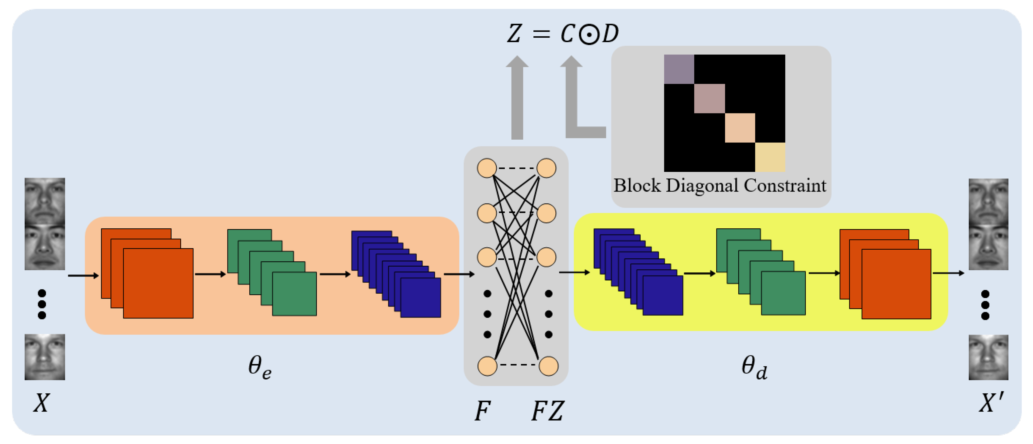
• A deep subspace clustering method based on an auto-encode is proposed, and block-diagonal constraints on representation matrix are used for better cluster performance.
• A separation strategy on the block diagonal constraint is proposed for more flexibility.
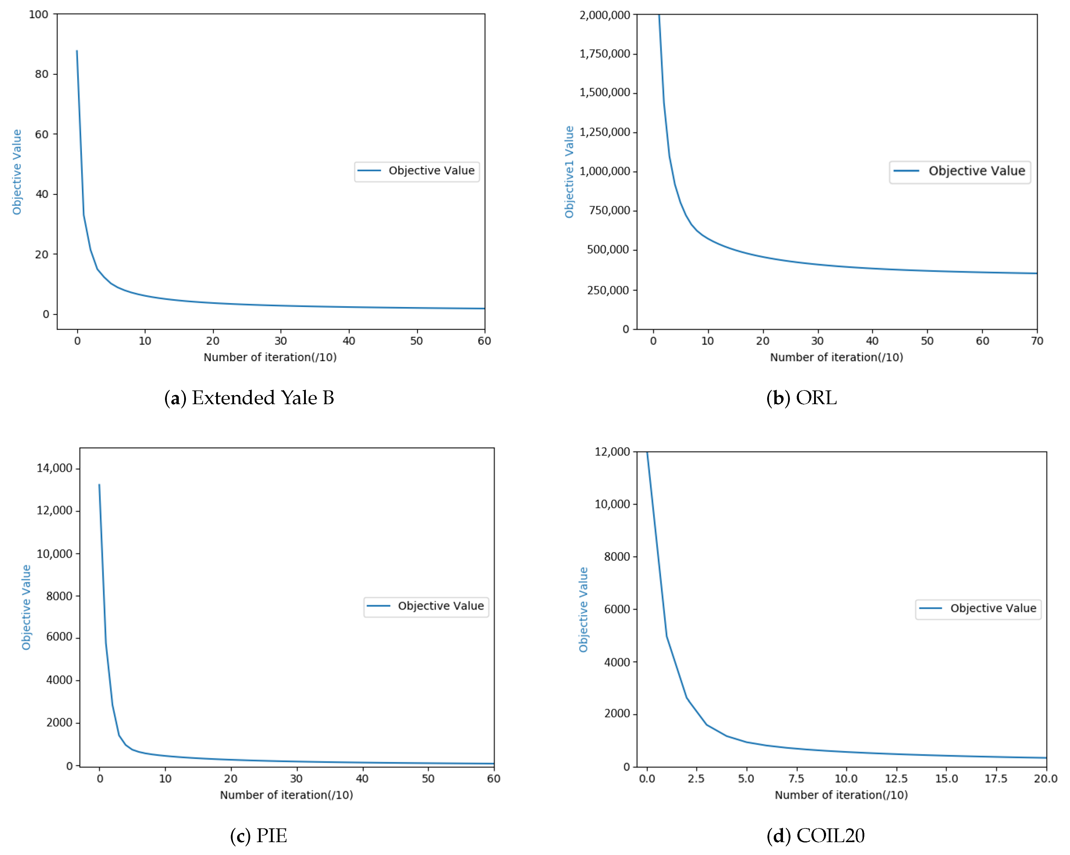
• Due to the existing of new block diagonal regularizer, an alternating optimization method to solve proposed model is developed.
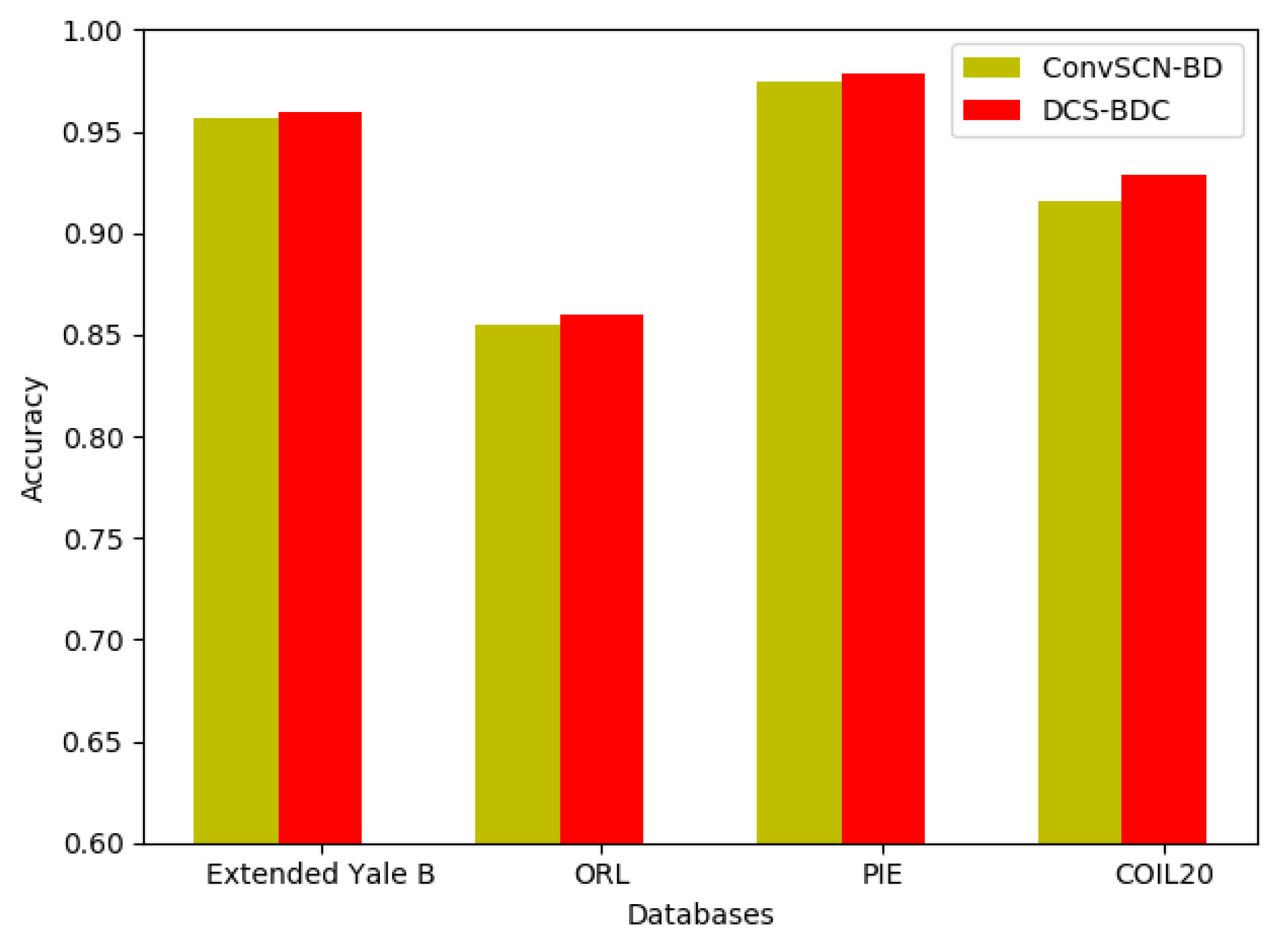
• The proposed DSC-BDC is evaluated on four databases, and the results demonstrate the effectiveness of our model.

The rest of this paper is organized as follows. Section 2 gives the proposed DSC-BDC model and optimization algorithm. Section 3 provides experimental results and analysis based on four public databases. Finally, the conclusions and future works are summarized in Section 4.

2. Deep Subspace Clustering Model with Block Diagonal Constraint

In this section, the details of the proposed Deep Subspace Clustering Model with Block Diagonal Constraint (DSC-BDC) are described. Then, the entire optimization algorithm is given. In addition, the relationship between the proposed model and related work is analyzed.

2.1. Model Formulation

Given the input samples set $X=\{x_1,x_2,\cdots ,x_N\}$, which consists of N samples. Each sample may be raw data or manually extracted features, such as images or extracted image features. As illustrated in Figure 1, our deep network model selects the convolutional auto-encoder as the basic framework and uses fully connected without bias and nonlinear activation as the self-expression layer. Let $\Theta$ denote the auto-encoder module parameters, which can be decomposed into encoder parameters ${\theta }_e$ and decoder parameters ${\theta }_d$. Z denotes the self-expression module parameters, which is the representation matrix. $F=\left\{f_1,f_2,\cdots ,f_N\right\}$ is the latent representation corresponding to $X=\left\{x_1,x_2,\cdots ,x_N\right\}$, which is learned by the encoder. Therefore, latent feature $f_i=\phi (x_i,{\theta }_e)$, $\phi (·)$ means to map the original data to latent feature. The output of decoder is $X^{{}^{\prime }}=\left\{x_1^{{}^{\prime }},x_2^{{}^{\prime }},\dots ,x_N^{{}^{\prime }}\right\}$, which is a function of $\tilde{\Theta }=\left\{\Theta ,Z\right\}$. The naive deep subspace clustering can be formulated as a minimization problem as follows:

$$\underset{\tilde{\Theta }}{min}\frac{1}{2}\parallel X-X^{{}^{\prime }}{\parallel }_F^2+\frac{1}{2}{\parallel F-FZ\parallel }_F^2+{\alpha }_1{\parallel Z\parallel }_p,$$

(1)

where ${\alpha }_1$ is a positive trade-off parameter that balances the terms of the objective function. Here, DSC-Net uses $\frac{1}{2}{\parallel F-FZ\parallel }_F^2$ to measure the self-expression errors, $\frac{1}{2}{\parallel X-X^{{}^{\prime }}\parallel }_F^2$ to calculate the reconstruction cost and ${\parallel Z\parallel }_p$ as a prior structure regularization of self-expressive representation Z, which is used to avoid trivial solution.

Subspace clustering methods based on self-expressive property firstly learn a representation matrix, and then spectral clustering is performed on the representation matrix to obtain the clustering result. Thus, the representation matrix plays an important role in spectral clustering. Whether it can truly reflect the similarity between data samples will directly affect the clustering performance. The ideal representation matrix in spectral clustering should have obvious block diagonal structure since all the inter-cluster affinities should be zero. To approximate such a structure, sparse or low-rank priors are adopted to the self-expressive representation matrix. there are two main types of constrained representation matrices: $l_1$ norm to pursue sparsity [17] and nuclear norm to pursue low-rankness [15]. However, these two constraints are too rough and cannot guarantee a good diagonal structure. Unlike these indirect structure priors, Lu et al. [20] firstly proposed block diagonal regularization terms to directly constrain the representation matrix as a block diagonal structure.

Theorem 1

[44]. For any $Z\ge 0$, $Z=Z^T$, the multiplicity k of the eigenvalue 0 of $L_Z$ equals the number of connected components (blocks) in Z, where $L_Z=D-Z$, D is a diagonal matrix with diagonal element $D_{ii}={\sum }_{i=1}^N{Z}_{ij}$.

This theorem provides theoretical support for the the block diagonal constraint. We can know with Theorem 1 that Z is k block diagonal ( which means that Z has k connected components) if and only if

$${\lambda }_i\left(L_Z\right)=\left\{\begin{array}{ccc}\hfill >0,& & i=1,\cdots ,N-k;\hfill \\ \hfill =0,& & i=N-k+1,\cdots ,N;\hfill \end{array}\right.$$

where ${\lambda }_i\left(L_Z\right)(i=1,\cdots ,N)$ are the eigenvalues of $L_Z$ in decreasing order. Thus, we can employ the sum of the k smallest eigenvalues of $L_Z$ as the k block diagonal regularizer, i.e.,

$${\parallel Z\parallel }_{\kappa }=\sum _{i=N-k+1}^N{\lambda }_i\left(L_Z\right).$$

(2)

Obviously, the representation matrix Z is k block diagonal when ${\parallel Z\parallel }_{\kappa }=0$. Thus, ${\parallel Z\parallel }_{\kappa }$ measures the k block diagonal degree of Z, and we can minimize ${\parallel Z\parallel }_{\kappa }$ for learning the representation Z with k block diagonal structure.

While introducing the above k block diagonal regularization in [20], we can rewrite the DSC-Net loss function as follows:

$$\underset{\tilde{\Theta }}{min}\frac{1}{2}\parallel X-X^{{}^{\prime }}{\parallel }_F^2+\frac{1}{2}{\parallel F-FZ\parallel }_F^2+{\alpha }_1{\parallel Z\parallel }_F^2+{\alpha }_2{\parallel Z\parallel }_{\kappa }.$$

(3)

We know that ${\parallel Z\parallel }_{\kappa }=0$ will cause a strict block diagonal structure, whose elements are zero except for the diagonal block elements. This is a strong constraint and will make the network over-fit and unstable for increasing error.

Therefore, this paper introduces a separation strategy to separate the self-expression matrix for providing more freedom to guarantee both the exact self-expression and approximating k block diagonal structure. Different from directly constraining Z, this separation strategy decomposes Z into C and D, and then we only constrain C with a block diagonal structure to relax the constraints. We define $Z=C\odot D$ to call for two distinct matrices, C and D, with the same size, here $Z_{ij}=D_{ij}·C_{ij}$, which denotes the element-wise product. We bound the magnitudes of C via the constraint $C\le C_{max}$, which is to avoid the magnitude of C dominating the other variables. For D, it is easy to see that $D_{ij}=0$ will make ${(C\odot D)}_{ij}=0$, even if $C_{ij}\ne 0$. Therefore, we use $D_{min}$ as the lower bound to constrain the elements in D. Motivated by the above idea, we improve DSC-Net model to our deep subspace clustering model with block diagonal constraint (DSC-BDC), which can be formulated as follows:

$$\begin{array}{cc}\hfill \underset{\tilde{\Theta },C,D}{min}& \frac{1}{2}\parallel X-X^{{}^{\prime }}{\parallel }_F^2+\frac{1}{2}{\parallel F-FZ\parallel }_F^2+\frac{{\alpha }_1}{2}{\parallel Z\parallel }_F^2\hfill \\ \hfill & +\frac{{\alpha }_2}{2}{\parallel Z-C\odot D\parallel }_F^2+\frac{{\alpha }_3}{2}{\parallel D\parallel }_F^2+{\alpha }_4{\parallel C\parallel }_{\kappa }\hfill \\ \hfill \mathrm{s}.\mathrm{t}.& C\in \mathcal{C},D\in \mathcal{D},\hfill \end{array}$$

(4)

where

$$\mathcal{C}=\{C\in {\mathbb{R}}^{N\times N}:0\le C\le C_{max},diag\left(C\right)=0,C=C^T\},$$

(5)

$$\mathcal{D}=\{D\in {\mathbb{R}}^{N\times N}:D_{ij}\ge D_{min}\}.$$

(6)

$Z\in {\mathbb{R}}^{N\times N}$ is the representation matrix corresponding to the subspace structure of X; $C\in {\mathbb{R}}^{N\times N}$ and $D\in {\mathbb{R}}^{N\times N}$ are obtained by matrix multiplication decomposition of representation matrix Z; and ${\alpha }_1,{\alpha }_2,{\alpha }_3,{\alpha }_4$ are the regular term parameters. The first term of objective function is the reconstruction errors of the auto-encoder network, the second term is the self-expression error and the third term is the regular term to avoid trivial solutions. For the last three items, ${\parallel Z-C\odot D\parallel }_F^2$ is the multiplicative decomposition term, ${\parallel D\parallel }_F^2$ is the regularization term and the template C is constrained as a block diagonal structure through the ${\parallel C\parallel }_{\kappa }$ term.

Thus, the representation matrix Z will be with an approximate block diagonal structure, and it is hoped this improves the clustering performance.

2.2. Model Optimization

According to Equation (2), the regularization term ${\parallel C\parallel }_{\kappa }$ means that the sum of k smallest eigenvalues of $L_C$ needs to be minimized, which is difficult to solve. However, according to the basic properties of the eigenvalues [20,45], the regularization term can be rewritten as:

$${\parallel C\parallel }_{\kappa }=\sum _{i=N-k+1}^N{\lambda }_i\left(L_C\right)=\underset{W}{min}\langle L_C,W\rangle \mathrm{s}.\mathrm{t}.W\in \mathcal{W},$$

(7)

where

$$\mathcal{W}=\{W\in {\mathbb{R}}^{N\times N}:0⪯W⪯I,tr\left(W\right)=k\}.$$

(8)

$L_C=D_C-(C+C^T)/2$, $D_C\in {\mathbb{R}}^{N\times N}$ is a diagonal matrix whose diagonal elements are ${\sum }_j(c_{ij}+c_{ji})/2$, $W^T=\left\{w_1,w_2,\dots ,w_N\right\}$, and $I\in {\mathbb{R}}^{N\times N}$ is the identity matrix. $\langle L_C,W\rangle$ denotes the inner product between the two matrices. Thus, Equation (4) can be rewritten as:

$$\begin{array}{cc}\hfill \underset{\Theta ,Z,C,D,W}{min}& \frac{1}{2}\parallel X-X^{{}^{\prime }}{\parallel }_F^2+\frac{1}{2}{\parallel F-FZ\parallel }_F^2+\frac{{\alpha }_1}{2}{\parallel Z\parallel }_F^2\hfill \\ \hfill & +\frac{{\alpha }_2}{2}{\parallel Z-C\odot D\parallel }_F^2+\frac{{\alpha }_3}{2}{\parallel D\parallel }_F^2\hfill \\ \hfill & +{\alpha }_4\langle L_C,W\rangle \hfill \\ \hfill \mathrm{s}.\mathrm{t}.& C\in \mathcal{C},D\in \mathcal{D},W\in \mathcal{W}.\hfill \end{array}$$

(9)

Obviously, the model (9) is non-convex optimization problems, which is difficult to solve directly. Therefore, we intend to employ the alternating direction method (ADM) [46] to alternatively optimize variables $\Theta$, Z, D, C and W.

Update$\Theta ,Z$: While all other variables C, D and W are fixed, we can update $\Theta$, Z by solving sub-problem (10)

$$\begin{array}{cc}\hfill \underset{\Theta ,Z}{min}& \frac{1}{2}\parallel X-X^{{}^{\prime }}{\parallel }_F^2+\frac{1}{2}{\parallel F-FZ\parallel }_F^2+\frac{{\alpha }_1}{2}{\parallel Z\parallel }_F^2\hfill \\ \hfill & +\frac{{\alpha }_2}{2}{\parallel Z-C\odot D\parallel }_F^2\hfill \\ \hfill \mathrm{s}.\mathrm{t}.& C\in \mathcal{C},D\in \mathcal{D}.\hfill \end{array}$$

(10)

It is worth noting that (10) is differentiable on $\Theta$ and Z, thus we use stochastic gradient descent to update $\Theta$ and Z.

Update D: When other variables are fixed, the corresponding sub-problem for D is then given by

$$\begin{array}{cc}\hfill \underset{D}{min}& \frac{{\alpha }_2}{2}{\parallel Z-C\odot D\parallel }_F^2+\frac{{\alpha }_3}{2}{\parallel D\parallel }_F^2\hfill \\ \hfill \mathrm{s}.\mathrm{t}.& D\in \mathcal{D}.\hfill \end{array}$$

(11)

The elements $D_{ij}$ are independent of each other. Thus, we can update $D_{ij}$ separately by the resulting sub-problem

$$\begin{array}{cc}\hfill \underset{D_{ij}}{min}& {(D_{ij}-\frac{{\alpha }_2{C}_{ij}{Z}_{ij}}{{\alpha }_3+{\alpha }_2{C}_{ij}^2})}^2\hfill \\ \hfill \mathrm{s}.\mathrm{t}.& D_{ij}\ge D_{min}\hfill \end{array}$$

(12)

Solving the above formula, it can be obtained that:

$$D_{ij}=\{\begin{array}{cc}\frac{{\alpha }_2{C}_{ij}{Z}_{ij}}{{\alpha }_3+{\alpha }_2{C}_{ij}^2}\hfill & \mathrm{if}\frac{{\alpha }_2{C}_{ij}{Z}_{ij}}{{\alpha }_3+{\alpha }_2{C}_{ij}^2}\ge D_{min};\hfill \\ D_{min}\hfill & \mathrm{otherwise}.\hfill \end{array}$$

(13)

We define $P=A^{\odot -1}B$, where the matrices A and B are different but have the same size. We have $P_{ij}=\frac{B_{ij}}{A_{ij}}$, which denotes the element-wise division. For convenience, the solution of (12) can be re-expressed as:

$$\begin{array}{c}\hfill {\mathsf{\Pi }}_{\mathcal{D}}{\left(({\alpha }_{2}C\odot C+{\alpha }_3)\right)}^{\odot -1}({\alpha }_{2}C\odot Z)),\end{array}$$

(14)

where

$${\mathsf{\Pi }}_{\mathcal{D}}{\left(S\right)}_{ij}=\left\{\begin{array}{cc}{S}_{ij}\hfill & \mathrm{if}{S}_{ij}\ge D_{min};\hfill \\ D_{min}\hfill & \mathrm{otherwise}.\hfill \end{array}\right.$$

(15)

Update C: Fix all other variables Z, $\Theta$, D and W to update C. The corresponding sub-problem for C is then given by

$$\begin{array}{cc}\hfill \underset{C}{min}& \frac{{\alpha }_2}{2}{\parallel Z-C\odot D\parallel }_F^2+{\alpha }_4\langle L_c,W\rangle \hfill \\ \hfill \mathrm{s}.\mathrm{t}.& C\in \mathcal{C}\hfill \end{array}$$

(16)

The solution of (16) can be re-expressed as:

$$\begin{array}{c}\hfill {\Pi }_{\mathcal{C}}\left(\tilde{C}\right),\end{array}$$

(17)

where

$$\begin{array}{cc}\hfill & {\tilde{C}}_{ij}=\left\{\begin{array}{cc}\frac{{\alpha }_2(D_{ij}{Z}_{ij}+D_{ji}{Z}_{ji})-{\alpha }_4({\overline{W}}_{ij}+{\overline{W}}_{ji})}{{\alpha }_2(D_{ij}^2+D_{ji}^2)}\hfill & \mathrm{if}i\ne j;\hfill \\ \mathbf{0}\hfill & \mathrm{otherwise},\hfill \end{array}\right.\hfill \\ \hfill & \overline{W}=diag\left(W\right)1^T-W,\hfill \\ \hfill & {\mathsf{\Pi }}_{\mathcal{C}}{\left(S\right)}_{ij}=\left\{\begin{array}{cc}max\{0,S_{ij}\}\hfill & \mathrm{if}{S}_{ij}\le C_{max};\hfill \\ C_{max}\hfill & \mathrm{otherwise}.\hfill \end{array}\right.\hfill \end{array}$$

(18)

To obtain a stable result, it is necessary to add a small positive number $ϵ$ to the denominator term, i.e., ${\alpha }_2(D_{ij}+D_{ji})+ϵ$. The proof of updating rule is provided in Appendix A.

Update W: Fixing all the other parameters, W can be solved from the following problem. Fix all other variables Z, $\Theta$, D and W to update C. The corresponding sub-problem for C is then given by:

$$\begin{array}{cc}\hfill \underset{W}{min}& \langle L_C,W\rangle \hfill \\ \hfill \mathrm{s}.\mathrm{t}.& W\in \mathcal{W}.\hfill \end{array}$$

(19)

Following Lu et al. [20], the optimal solution is defined as

$$\begin{array}{c}\hfill W=V{V}^T,\end{array}$$

(20)

where $V=\left\{v_1,v_2,\dots ,v_k\right\}$ and $v_i$ is an eigenvector associated with the ith smallest eigenvalue of $L_C$.

Based on the above analysis, we summarize the optimization procedure for our model in Algorithm 1.

Algorithm 1 Optimization algorithm for DSC-BDC

Input:  X, ${\alpha }_1$, ${\alpha }_2$, ${\alpha }_3$, $C_{max}$, $D_{min}$. Output:  Z, C, D. 1: $D_{ij}\leftarrow D_{min}$; 2: $W\leftarrow I$; 3: $C\leftarrow 0$; 4: while not converged do 5:    $iter\leftarrow iter+1$; 6:    $Z_{old}\leftarrow Z$; 7:    $D_{old}\leftarrow D$; 8:    $C_{old}\leftarrow C$; 9:    $W_{old}\leftarrow W$; 10:   Update $\mathbf{Z}$ with (10); 11:   Update $\mathbf{D}$ with (14); 12:   Update $\mathbf{C}$ with (17); 13:   Update $\mathbf{W}$ with (20). 14: end while

According to the previous sub-problems, we give the complexity analysis as follows: For updating Z, the computational complexity in network is $O\left(n^2\right)$ at a time. Obviously, for updating C and D, one needs $O\left(n^2\right)$ operations. For updating W, one needs $O\left(n^3\right)$ operations to perform the eigenvalue decomposition. Thus, it is easy to obtain the total complexity of the proposed algorithm at each iteration by summing all the steps. We conclude that the computational complexity of our proposed method is then $\mathcal{O}\left(n^3\right)$.

3. Experiments

In this section, we carry out a large number of experiments to evaluate DSC-BDC and compare it with several excellent methods published in recent years to verify the performance of the proposed algorithm. In addition, we give a particular explanation about the parameter settings, the pre-trained models and the fine-tuning procedures used in our experiments.

All algorithms were coded with Python 3.6 with Pytorch and were run on the platform of Windows 10 with Intel Core i7-8550U 1.80GHz CPU and 8G RAM.

3.1. Experimental Settings

3.1.1. Baseline Algorithms

In our experiments, the proposed DSC-BDC is compared with following algorithms consisting of subspace clustering in the raw space and latent space: Sparse Subspace Clustering (SSC) [17], SSC with the pre-trained auto-encoder features (AE+SSC), Low Rank Representation (LRR) [15], Low Rank Subspace Clustering (LRSC) [18], Efficient Dense Subspace Clustering (EDSC) [47], EDSC with the pre-trained auto-encoder features (AE+EDSC), Low-Rank Kernel Subspace Clustering (LR-kernel SC) [48], Subspace Clustering by Block Diagonal Representation (BDR) [20], Deep Subspace Clustering Networks (DSC-Net) [30] and Convolutional Subspace Clustering Network With Block Diagonal Prior (ConvSCN-BD) [49].

For DSC-Net method, we run the same epochs as DSC-BDC and report the last epoch performance. For ConvSCN-BD, we use the default setting as the authors’ suggestion. In the experimental setting, all the methods involve k-means clustering method for the final clustering results. The initialization of solution heavily influences the performance of k-means. Thus, we run it 20 times, and the average performance and standard deviation are reported.

3.1.2. Databases

We evaluated DSC-BDC method on four public databases, i.e., the Extended Yale B, ORL and PIE face image databases and the COIL20 object image database. A brief introduction of these databases is listed in

Table 1. The detailed information about used databases.

Database	Sample Number	Size	Class
Extended Yale B	882	32 × 32	14
ORL	400	32 × 32	40
PIE	1428	32 × 32	68
COIL20	1440	32 × 32	20

.

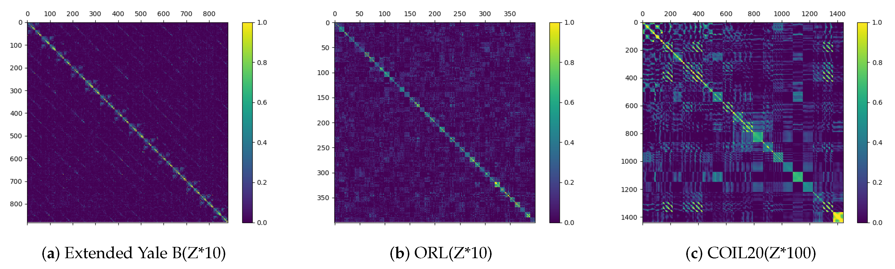
• Extended Yale B database: Extended Yale B [50] consists of 2414 frontal face pictures of 38 subjects under 9 poses and 64 illumination conditions. For each subject, there are 64 images. Each cropped face image consists of $192\times 168$ pixels. In the experiment, we use the first 14 subjects with a total of 882 images for testing. All images are resized to $32\times 32$ pixels.
• ORL database: The ORL database [51] is composed of 400 photographs of size $112\times 92$ from 40 different individuals where each subject has 10 images taken under diverse variation of lighting conditions, poses and facial expressions. Following the literature, we downsample the images from their raw size to $32\times 32$.
• PIE database: This face image database [52,53] consists of 40,000 photographs of 68 individuals, illustrating 13 pose conditions for each person, 43 with illumination levels and four expressions. It is worth noting that the pictures in the PIE database are all color pictures. In the experiment, we select 1428 samples of 68 subjects, and the sample size is 32 × 32. For convenience, the color images are converted to gray-scale images.
• COIL20 database: COIL20 [54] is a color object image database with 1440 images of 20 objects. Each object was placed on a turntable against a black background, and 72 images were taken at pose intervals of 5 degrees. For convenience, the color images are converted to gray-scale images; however, this is not necessary. The images are down-sampled to 32 × 32.

3.1.3. Training Strategy and Parameter Settings

During model training, we first use the convolutional autoencoder as the pre-training model to initialize the network parameters $\Theta$, and then the $\Theta$ is used as the initial parameter of fine-tuning.

During pre-training, we remove the self-expression module, and the pre-trained network degenerates into the simplest convolutional auto-encoder. The output $X^{{}^{\prime }}$ of the decoder is only a function of $\left\{{\theta }_e,{\theta }_d\right\}$. We pre-train the network by minimizing the following reconstruction error:

$$\mathcal{L}({\theta }_e,{\theta }_d)=\frac{1}{2}{\parallel X-X^{{}^{\prime }}\parallel }_F^2.$$

(21)

When the convolutional auto-encoder is trained, we add a self-expression module, and at the same time extract the parameters of the self-expression module, which is the coefficient matrix $Z\in {\mathbb{R}}^{N\times N}$. The output $X^{{}^{\prime }}$ of the decoder is only a function of $\left\{{\theta }_e,{\theta }_s,{\theta }_d\right\}$. This is the deep subspace clustering network, which can be trained by minimizing the following loss:

$$\begin{array}{c}\hfill \mathcal{L}({\theta }_e,{\theta }_s,{\theta }_d)=\frac{1}{2}\parallel X-X^{{}^{\prime }}{\parallel }_F^2+\frac{1}{2}{\parallel F-FZ\parallel }_F^2+\frac{{\alpha }_1}{2}{\parallel Z\parallel }_F^2.\end{array}$$

(22)

For the convolutional layers, the stride of kernel is 2 in both horizontal and vertical directions, and nonlinear activation is the Rectified Linear Unit (ReLU). At the same time, the learning rate is set as 0.001 in all experiments.

For all databases, the kernel size in convolutional layers is set to 3 × 3. For Extended Yale B database, we set the channels as 20. In the fine-tuning stage, we set ${\alpha }_1=2$, ${\alpha }_2=40$, ${\alpha }_3=1.25$, ${\alpha }_4=2$ and $ϵ=1\times {10}^{-6}$ and run 450 epochs for DSC-BDC. For ORL database, we set the channels as 3–3–5–5–3–3. In the fine-tuning stage, we set $epoch=700$, ${\alpha }_1=2$, ${\alpha }_2=40$, ${\alpha }_3=1.25$, ${\alpha }_4=2$ and $ϵ=1\times {10}^{-6}$. In addition, for PIE database, we set the number of channels to 20 and set $epoch=450$, ${\alpha }_1=1$, ${\alpha }_2=40$, ${\alpha }_3=1$, ${\alpha }_4=2$ and $ϵ=1\times {10}^{-6}$. On COIL20 database, the number of channels is 15, and the parameters are consistent with PIE databases except that $epoch=40$.

3.2. Experimental Results and Analysis

We employ three popular metrics to evaluate the clustering performance of all compared algorithms: Accuracy (ACC), Normalized Mutual Information (NMI) and Adjusted Rand Index (ARI). With the block-diagonal representation Z, we calculate the affinity matrix $A=\frac{\left|Z\right|+|Z^T|}{2}$. Then, the clustering result is obtained by performing the spectral clustering method on affinity matrix A.

The experimental results of different methods on the Extended Yale B, ORL, PIE and COIL20 databases are shown in the

Table 2. Clustering performance of different algorithms on the Extended Yale B database.

Methods	ACC	NMI	ARI
LRR	0.5696 ± 0.0104	0.5535 ± 0.0060	0.2164 ± 0.0149
LSR	0.5652 ± 0.0100	0.5548 ± 0.0052	0.2175 ± 0.0092
SSC	0.5412 ± 0.0103	0.5336 ± 0.0036	0.2456 ± 0.0162
AE+SSC	0.5778 ± 0.0400	0.5793 ± 0.0096	0.1751 ± 0.0373
LR-kernel SC	0.8016 ± 0.0101	0.8461 ± 0.0013	0.7352 ± 0.0108
EDSC	0.6138 ± 0.0196	0.5868 ± 0.0093	0.2722 ± 0.0220
AE+EDSC	0.6061 ± 0.0228	0.5910 ± 0.0163	0.2694 ± 0.0196
BDR	0.7253 ± 0.0111	0.7103 ± 0.0030	0.4927 ± 0.0046
DSC-Net	0.9548 ± 0.0003	0.9227 ± 0.0004	0.8987 ± 0.0008
ConvSCN-BD	0.9559 ± 0.0010	0.9260 ± 0.0008	0.9035 ± 0.0012
Ours	0.9592 ± 0.0008	0.9301 ± 0.0010	0.9060 ± 0.0018

,

Table 3. Clustering performance of different algorithms on the ORL database.

Methods	ACC	NMI	ARI
LRR	0.6775 ± 0.0186	0.7881 ± 0.0160	0.4305 ± 0.0348
LSR	0.6800 ± 0.0260	0.7940 ± 0.0109	0.4288 ± 0.0473
SSC	0.7504 ± 0.0141	0.8578 ± 0.0071	0.5988 ± 0.0225
AE+SSC	0.7383 ± 0.0215	0.8428 ± 0.0088	0.5915 ± 0.0252
LR-kernel SC	0.7185 ± 0.0194	0.8540 ± 0.0068	0.6088 ± 0.0200
EDSC	0.6938 ± 0.0255	0.8089 ± 0.0126	0.5043 ± 0.0305
AE+EDSC	0.6974 ± 0.0171	0.8139 ± 0.0109	0.5026 ± 0.0365
BDR	0.7204 ± 0.0192	0.8350 ± 0.0117	0.4662 ± 0.0471
DSC-Net	0.8463 ± 0.0080	0.9172 ± 0.0021	0.7878 ± 0.0062
ConvSCN-BD	0.8360 ± 0.0090	0.9149 ± 0.0059	0.7791 ± 0.0131
Ours	0.8505 ± 0.0079	0.9182 ± 0.0027	0.7932 ± 0.0037

,

Table 4. Clustering performance of different algorithms on the PIE database.

Methods	ACC	NMI	ARI
LRR	0.7392 ± 0.0206	0.8808 ± 0.0079	0.6041 ± 0.0239
LSR	0.7484 ± 0.0212	0.8812 ± 0.0100	0.5799 ± 0.0404
SSC	0.7652 ± 0.0184	0.9060 ± 0.0070	0.6510 ± 0.0285
AE+SSC	0.7820 ± 0.0234	0.9191 ± 0.0066	0.6850 ± 0.0204
LR-kernel SC	0.7520 ± 0.0174	0.9341 ± 0.0043	0.7238 ± 0.0199
EDSC	0.8148 ± 0.0143	0.9073 ± 0.0060	0.6231 ± 0.0641
AE+EDSC	0.8251 ± 0.0184	0.9164 ± 0.0062	0.6433 ± 0.0545
BDR	0.8094 ± 0.0200	0.9130 ± 0.0086	0.5980 ± 0.0712
DSC-Net	0.9686 ± 0.0072	0.9911 ± 0.0052	0.9620 ± 0.0120
ConvSCN-BD	0.9732 ± 0.0203	0.9890 ± 0.0041	0.9723 ± 0.0211
Ours	0.9760 ± 0.0035	0.9960 ± 0.0046	0.9807 ± 0.0031

and

Table 5. Clustering performance of different algorithms on the COIL20 database.

Methods	ACC	NMI	ARI
LRR	0.6887 ± 0.0190	0.7714 ± 0.0097	0.5873 ± 0.0150
LSR	0.6871 ± 0.0142	0.7683 ± 0.0097	0.5927 ± 0.0204
SSC	0.7898 ± 0.0292	0.8917 ± 0.0117	0.0.6546 ± 0.0820
AE+SSC	0.8863 ± 0.0113	0.9205 ± 0.0074	0.7979 ± 0.0278
LR-kernel SC	0.6268 ± 0.0083	0.8056 ± 0.0035	0.5568 ± 0.0154
EDSC	0.8514 ± 0.0000	-	-
AE+EDSC	0.8521 ± 0.0000	-	-
BDR	0.7549 ± 0.0000	0.8862 ± 0.0000	0.6249 ± 0.0000
DSC-Net	0.9004 ± 0.0288	0.9562 ± 0.0095	0.8765 ± 0.0384
ConvSCN-BD	0.9160 ± 0.0037	0.9613 ± 0.0002	0.8989 ± 0.0032
Ours	0.9174 ± 0.0010	0.9632 ± 0.0021	0.8944 ± 0.0037

. The bold numbers in the table are the best results, and the short line means that some evaluation metrics of some methods are not shown.

From the results in Table 2, Table 3, Table 4 and Table 5, the following observations can be found: (1) Overall, DSC-BDC achieves competitive and stable performance compared to most baselines on all databases. Taking the Extended Yale B database as an example, DSC-BDC outperforms the other best method DSC-Net by $0.44\%$, $0.74\%$ and $0.73\%$ in terms of ACC, NMI and ARI, respectively. (2) Observing the experimental results of SSC and AE+SSC, it can be seen that, in most cases, the latter has higher accuracy, which indicates that deep networks can better extract nonlinear data features to improve the clustering effect. (3) Comparing BDR and DSC-Net, we can see that deep networks have powerful representation learning ability. Compared with the clustering results obtained by the BDR method (no network) with block diagonal structure constraints, DSC-Net does not strictly require the representation matrix structure and also obtained good clustering performance. (4) Our DSC-BDC framework achieves better performance than DSC-Net. The reason might be that a direct block diagonal regularizer is more effective than regularization using indirect structure priors in self-expression.

For visually intuition, we show the corresponding derived representation matrix, as a clearer block diagonal structure of the representation matrix results in higher clustering performance. We show the three databases (Extended Yale B, ORL and COIL20) in Figure 2. Clearly, the representation matrix Z has apparent block diagonal structure. We next explore the advantages of the method using the separation strategy (DSC-BDC) over the method without the separation strategy (ConvSCN-BD). We plot the accuracy of different databases in Figure 3. This implies the effectiveness of the separation strategy.

We verify the convergence of DSC-BDC through the experiment of drawing convergence curves. The convergence curves of the four public databases are shown in Figure 4. In each subfigure, we define the horizontal axis to represent the number of iteration steps and the vertical axis to correspond to the value of termination criterion. It can be observed that DSC-BDC algorithm can converge with few iteration steps.

4. Conclusions

We propose a Deep Subspace Clustering with Block Diagonal Constraint (DSC-BDC) model, in which the coefficient representation matrix is loosely block diagonally constrained by means of a separation strategy. Furthermore, for solving the joint optimization problem, the algorithm alternately updates the auto-encoder module, representation matrix parameters and matrix decomposition module parameters. On the other side, by using the block diagonal constraint, we can learn a better representation matrix from the self-expression coefficient to obtain more stable and excellent clustering performance. From the experiments on four benchmark image datasets, we can conclude that our model is effective and promising. In future work, we will extend our model to deep multi-view subspace clustering. We assume that there is consistent information among different views of multi-view data and that each view has view-specific information [21,24,45]. We impose a separation strategy on multi-view data, so that each view shares consistent structural information on the premise of maintaining its view-specific information. At the same time, the block diagonal constraint is constrained to the shared information (matrix) to improve the clustering performance, and we use the network to learn the variables of the separation strategy module instead of solving the variables through the alternating iterative algorithm.

References

1. Hong, W.; Wright, J.; Huang, K.; Ma, Y. Multiscale Hybrid Linear Models for Lossy Image Representation. IEEE Trans. Image Process. 2006, 15, 3655–3671. [Google Scholar] [CrossRef] [PubMed]
2. Liu, G.; Lin, Z.; Yan, S.; Sun, J.; Yu, Y.; Ma, Y. Robust Recovery of Subspace Structures by Low-Rank Representation. IEEE Trans. Pattern Anal. Mach. Intell. 2013, 35, 171–184. [Google Scholar] [CrossRef] [PubMed] [Green Version]
3. Eldar, Y.C.; Mishali, M. Robust Recovery of Signals From a Structured Union of Subspaces. IEEE Trans. Inf. Theory 2009, 55, 5302–5316. [Google Scholar] [CrossRef] [Green Version]
4. Cao, X.; Zhang, C.; Fu, H.; Liu, S.; Zhang, H. Diversity-induced Multi-view Subspace Clustering. In Proceedings of the IEEE Conference on Computer Vision and Pattern Recognition, Boston, MA, USA, 7–12 June 2015; pp. 586–594. [Google Scholar]
5. Zhang, C.; Fu, H.; Liu, S.; Liu, G.; Cao, X. Low-Rank Tensor Constrained Multiview Subspace Clustering. IEEE Int. Conf. Comput. Vis. 2015, 1582–1590. [Google Scholar]
6. Pham, D.; Saha, B.; Phung, D.Q.; Venkatesh, S. Improved Subspace Clustering via Exploitation of Spatial Constraints. In Proceedings of the IEEE Conference on Computer Vision and Pattern Recognition, Providence, RI, USA, 16–21 June 2012; pp. 550–557. [Google Scholar]
7. Rao, S.R.; Tron, R.; Vidal, R.; Ma, Y. Motion Segmentation in the Presence of Outlying, Incomplete, or Corrupted Trajectories. IEEE Trans. Pattern Anal. Mach. Intell. 2010, 32, 1832–1845. [Google Scholar] [CrossRef]
8. Aldroubi, A.; Sekmen, A. Nearness to Local Subspace Algorithm for Subspace and Motion Segmentation. IEEE Signal Process. Lett. 2012, 19, 704–707. [Google Scholar] [CrossRef] [Green Version]
9. Tari, L.; Baral, C.; Kim, S. Fuzzy C-means Clustering with Prior Biological Knowledge. J. Biomed. Inform. 2009, 42 1, 74–81. [Google Scholar] [CrossRef] [Green Version]
10. Militello, C.; Vitabile, S.; Rundo, L.; Russo, G.; Midiri, M.; Gilardi, M. A Fully Automatic 2D Segmentation Method for Uterine Fibroid in MRgFUS Treatment Evaluation. Comput. Biol. Med. 2015, 62, 277–292. [Google Scholar] [CrossRef]
11. Parsons, L.; Haque, E.; Liu, H. Subspace Clustering for High Dimensional Data: A Review. ACM Sigkdd Explor. Newsl. 2004, 6, 90–105. [Google Scholar] [CrossRef]
12. Agrawal, R.; Gehrke, J.; Gunopulos, D.; Raghavan, P. Automatic Subspace Clustering of High Dimensional Data for Data Mining Applications. In Proceedings of the International Conference on Management of Data, Seattle, WA, USA, 2–4 June 1998; pp. 94–105. [Google Scholar]
13. Elhamifar, E.; Vidal, R. Sparse Subspace Clustering: Algorithm, Theory, and Applications. IEEE Trans. Pattern Anal. Mach. Intell. 2013, 35, 2765–2781. [Google Scholar] [CrossRef] [Green Version]
14. Chen, G.; Lerman, G. Spectral Curvature Clustering (SCC). Int. J. Comput. Vis. 2009, 81, 317–330. [Google Scholar] [CrossRef] [Green Version]
15. Liu, G.; Lin, Z.; Yu, Y. Robust Subspace Segmentation by Low-Rank Representation. In Proceedings of the International Conference on Machine Learning, Haifa, Israel, 21–24 June 2010; pp. 663–670. [Google Scholar]
16. Lu, C.; Min, H.; Zhao, Z.; Zhu, L.; Huang, D.; Yan, S. Robust and Efficient Subspace Segmentation via Least Squares Regression. In Proceedings of the European Conference on Computer Vision, Florence, Italy, 7–13 October 2012; pp. 347–360. [Google Scholar]
17. Elhamifar, E.; Vidal, R. Sparse Subspace Clustering. In Proceedings of the IEEE Conference on Computer Vision and Pattern Recognition, Miami, FL, USA, 20–25 June 2009; pp. 2790–2797. [Google Scholar]
18. Vidal, R.; Favaro, P. Low Rank Subspace Clustering (LRSC). Pattern Recognit. Lett. 2014, 43, 47–61. [Google Scholar] [CrossRef] [Green Version]
19. Feng, J.; Lin, Z.; Xu, H.; Yan, S. Robust Subspace Segmentation with Block-diagonal Prior. In Proceedings of the IEEE Conference on Computer Vision and Pattern Recognition, Columbus, OH, USA, 23–28 June 2014; pp. 3818–3825. [Google Scholar]
20. Lu, C.; Feng, J.; Lin, Z.; Mei, T.; Yan, S. Subspace Clustering by Block Diagonal Representation. IEEE Trans. Pattern Anal. Mach. Intell. 2019, 41, 487–501. [Google Scholar] [CrossRef] [Green Version]
21. Guo, J.; Yin, W.; Sun, Y.; Hu, Y. Multi-View Subspace Clustering With Block Diagonal Representation. IEEE Access 2019, 7, 84829–84838. [Google Scholar] [CrossRef]
22. Wang, Y.; Xu, H.; Leng, C. Provable Subspace Clustering: When LRR Meets SSC. In Proceedings of the Neural Information Processing Systems, Daegu, Korea, 3–7 November 2013; pp. 64–72. [Google Scholar]
23. Ji, P.; Salzmann, M.; Li, H. Shape Interaction Matrix Revisited and Robustified: Efficient Subspace Clustering with Corrupted and Incomplete Data. In Proceedings of the IEEE International Conference on Computer Vision, Santiago, Chile, 7–13 December 2015; pp. 4687–4695. [Google Scholar]
24. Yang, Z.; Xu, Q.; Zhang, W.; Cao, X.; Huang, Q. Split Multiplicative Multi-View Subspace Clustering. IEEE Trans. Image Process. 2019, 28, 5147–5160. [Google Scholar] [CrossRef]
25. Chen, G.; Atev, S.; Lerman, G. Kernel Spectral Curvature Clustering (KSCC). In Proceedings of the IEEE International Conference on Computer Vision, Kyoto, Japan, 27 September–4 October 2009; pp. 765–772. [Google Scholar]
26. Patel, V.M.; Van Nguyen, H.; Vidal, R. Latent Space Sparse Subspace Clustering. In Proceedings of the IEEE International Conference on Computer Vision, Sydney, Australia, 1–8 December 2013; pp. 225–232. [Google Scholar]
27. Patel, V.M.; Vidal, R. Kernel Sparse Subspace Clustering. In Proceedings of the IEEE International Conference on Image Processing, Paris, France, 27–30 October 2014; pp. 2849–2853. [Google Scholar]
28. Yin, M.; Guo, Y.; Gao, J.; He, Z.; Xie, S. Kernel Sparse Subspace Clustering on Symmetric Positive Definite Manifolds. In Proceedings of the IEEE Conference on Computer Vision and Pattern Recognition, Las Vegas, NV, USA, 27–30 June 2016; pp. 5157–5164. [Google Scholar]
29. Peng, X.; Xiao, S.; Feng, J.; Yau, W.; Yi, Z. Deep Subspace Clustering with Sparsity Prior. In Proceedings of the International Joint Conference on Artificial Intelligence, New York, NY, USA, 9–15 July 2016; pp. 1925–1931. [Google Scholar]
30. Ji, P.; Zhang, T.; Li, H.; Salzmann, M.; Reid, I. Deep Subspace Clustering Networks. In Proceedings of the Conference and Workshop on Neural Information Processing Systems, Long Beach, CA, USA, 4–9 December 2017; pp. 24–33. [Google Scholar]
31. Peng, X.; Feng, J.; Xiao, S.; Yau, W.; Zhou, J.T.; Yang, S. Structured AutoEncoders for Subspace Clustering. IEEE Trans. Image Process. 2018, 27, 5076–5086. [Google Scholar] [CrossRef] [PubMed]
32. Zhang, J.; Li, C.; You, C.; Qi, X.; Zhang, H.; Guo, J.; Lin, Z. Self-Supervised Convolutional Subspace Clustering Network. In Proceedings of the IEEE Conference on Computer Vision and Pattern Recognition, Long Beach, CA, USA, 16–20 June 2019; pp. 5473–5482. [Google Scholar]
33. Zhang, T.; Ji, P.; Harandi, M.; Huang, W.; Li, H. Neural Collaborative Subspace Clustering. In Proceedings of the International Conference on Machine Learning, Long Beach, CA, USA, 10–15 June 2019; pp. 7384–7393. [Google Scholar]
34. Zhou, P.; Hou, Y.; Feng, J. Deep Adversarial Subspace Clustering. In Proceedings of the IEEE Conference on Computer Vision and Pattern Recognition, Salt Lake City, UT, USA, 18–23 June 2018; pp. 1596–1604. [Google Scholar]
35. Yang, S.; Zhu, W.; Zhu, Y. Residual Encoder-Decoder Network for Deep Subspace Clustering. In Proceedings of the 2020 IEEE International Conference on Image Processing (ICIP), Abu Dhabi, UAE, 25–28 October 2020. [Google Scholar]
36. Peng, X.; Zhu, H.; Feng, J.; Shen, C.; Zhang, H.; Zhou, J.T. Deep Clustering With Sample-Assignment Invariance Prior. IEEE Trans. Neural Netw. Learn. Syst. 2020, 31, 4857–4868. [Google Scholar] [CrossRef] [PubMed]
37. Mishra, D.; Jayendran, A.; Prathosh, A.P. Effect of the Latent Structure on Clustering with GANs. IEEE Signal Process. Lett. 2020, 27, 900–904. [Google Scholar] [CrossRef]
38. Mukherjee, S.; Asnani, H.; Lin, E.; Kannan, S. ClusterGAN: Latent Space Clustering in Generative Adversarial Networks. arXiv 2019, arXiv:1809.03627. [Google Scholar] [CrossRef]
39. Zhao, S.; Song, J.; Ermon, S. InfoVAE: Information Maximizing Variational Autoencoders. arXiv 2017, arXiv:1706.02262. [Google Scholar]
40. Han, C.; Murao, K.; Noguchi, T.; Kawata, Y.; Uchiyama, F.; Rundo, L.; Nakayama, H.; Satoh, S. Learning More with Less: Conditional PGGAN-based Data Augmentation for Brain Metastases Detection Using Highly-Rough Annotation on MR Images. In Proceedings of the 28th ACM International Conference on Information and Knowledge Management, Beijing, China, 3–7 November 2019. [Google Scholar]
41. Kingma, D.P.; Welling, M. Auto-Encoding Variational Bayes. arXiv 2014, arXiv:1312.6114. [Google Scholar]
42. Wolterink, J.; Leiner, T.; Viergever, M.; Išgum, I. Generative Adversarial Networks for Noise Reduction in Low-Dose CT. IEEE Trans. Med. Imaging 2017, 36, 2536–2545. [Google Scholar] [CrossRef]
43. Masci, J.; Meier, U.; Ciresan, D.C.; Schmidhuber, J. Stacked Convolutional Auto-Encoders for Hierarchical Feature Extraction. In International Conference on Artificial Neural Networks; Springer: Berlin/Heidelberg, Germany, 2011. [Google Scholar]
44. Chung, F.R.; Graham, F.C. Spectral Graph Theory; Number 92; American Mathematical Society: Providence, RI, USA, 1997. [Google Scholar]
45. Kheirandishfard, M.; Zohrizadeh, F.; Kamangar, F. Multi-Level Representation Learning for Deep Subspace Clustering. In Proceedings of the IEEE Winter Conference on Applications of Computer Vision (WACV), Snowmass Village, CO, USA, 1–5 March 2020. [Google Scholar]
46. Lin, Z.; Liu, R.; Su, Z. Linearized Alternating Direction Method with Adaptive Penalty for Low-Rank Representation. Adv. Neural Inf. Process. Syst. 2011, 612–620. [Google Scholar]
47. Ji, P.; Salzmann, M.; Li, H. Efficient Dense Subspace Clustering. In Proceedings of the Workshop on Applications of Computer Vision, Steamboat Springs, CO, USA, 24–26 March 2014; pp. 461–468. [Google Scholar]
48. Ji, P.; Reid, I.; Garg, R.; Li, H.; Salzmann, M. Low-Rank Kernel Subspace Clustering. arXiv 2017, arXiv:1707.04974. [Google Scholar]
49. Zhang, J.; Li, C.; Du, T.; Zhang, H.; Guo, J. Convolutional Subspace Clustering Network with Block Diagonal Prior. IEEE Access 2020, 8, 5723–5732. [Google Scholar] [CrossRef]
50. Georghiades, A.S.; Belhumeur, P.N.; Kriegman, D.J. From Few to Many: Illumination Cone Models for Face Recognition under Variable Lighting and Pose. IEEE Trans. Pattern Anal. Mach. Intell. 2001, 23, 643–660. [Google Scholar] [CrossRef] [Green Version]
51. Samaria, F.S.; Harter, A. Parameterisation of a Stochastic Model for Human Face Identification. In Proceedings of the 1994 IEEE Workshop on Applications of Computer Vision, Sarasota, FL, USA, 5–7 December 1994; pp. 138–142. [Google Scholar]
52. Fan, C.N.; Zhang, F. Homomorphic Filtering Based Illumination Normalization Method for Face Recognition. Pattern Recognit. Lett. 2011, 32, 1468–1479. [Google Scholar] [CrossRef]
53. Sim, T.; Baker, S.; Bsat, M. The CMU Pose, Illumination, and Expression (PIE) Database. In Proceedings of the Fifth IEEE International Conference on Automatic Face Gesture Recognition, Washington, DC, USA, 20–21 May 2002; pp. 53–58. [Google Scholar]
54. Nene, S.A.; Nayar, S.K.; Murase, H. Columbia Object Image Library (COIL-20); Department of Computer Science, Columbia University: New York, NY, USA, 1996. [Google Scholar]
Figure 1. Architecture of the proposed Deep Subspace Clustering with Block Diagonal Constraint (DSC-BDC). It consists of mainly three modules: (a) the convolutional encoder module is used to extract convolutional features, and the parameter is marked as θ e ; (b) the convolutional decoder module is used with the encoder module to initialize the convolutional module, and the parameter is marked as θ d ; and (c) the self-expression module with indirectly block diagonal constraint is used to learn a better representation matrix from the self-expression coefficients, by applying a separation strategy to the representation matrix.
Applsci 10 08942 g001
Figure 2. Visualization of the representation matrices based on Extended Yale B, ORL and COIL20. For the convenience of observation, for different database, we multiply the Z by 10, 10 and 100, respectively.
Applsci 10 08942 g002
Figure 3. The accuracy comparison of the method using the separation strategy (DSC-BDC) and the method without the separation strategy (ConvSCN-BD).
Applsci 10 08942 g003
Figure 4. Convergence curve of the proposed algorithm on the four databases.
Applsci 10 08942 g004