Remaining Useful Life Estimation of Bearings Using Data-Driven Ridge Regression

Abstract

Predicting the remaining useful life (RUL) of mechanical bearings is a challenging industrial task since RUL can differ even for the same equipment due to many uncertainties such as operating condition, model inaccuracy, and sensory noise in various industrial applications. This paper proposes the RUL prediction method combining analytical model-based and data-driven approaches to forecast when a failure will occur based on the time series data of bearings. Feature importance ranking and principal component analysis construct a reliable and predictable health indicator from various statistical time, frequency, and time–frequency domain features of the observed signal. The adaptive sliding window method then optimizes the parameters of the degradation model based on the ridge regression of the time series sequence with the sliding window. The proposed adaptive scheme provides significant performance improvement in terms of the RUL estimation accuracy and robustness against the possible errors of the degradation model compared to the traditional Bayesian approaches.

1. Introduction

Modern industrial companies must continuously maintain their production resources by using appropriate maintenance strategies to improve availability, reliability, and safety while reducing their maintenance costs [1,2,3]. In this domain, predictive maintenance is a promising research direction because it enables manufacturers to monitor the working condition of machinery and diagnose faults or predict the next failure [4,5]. While the interventions are conducted after the failure occurs in conventional corrective maintenance, it is executed according to the predicted health condition of the equipment in predictive maintenance [6].

The bearing prevents direct metal to metal contact between multiple elements of most motor-driven machines for various industrial applications [7,8]. Besides, it reduces energy consumption as sliding motion is replaced with low friction rolling. The faults of the rolling element bearings result in significant machinery failures because it incurs friction, heat, and, ultimately, the wear and tear of parts. Predicting the remaining useful life (RUL) of bearings is one of the major goals of predictive maintenance for mechanical systems [1]. The RUL of a system is the length of remaining useful time before it is repaired or replaced. Engineers can schedule maintenance, optimize operating efficiency, and avoid unplanned downtime based on the RUL estimation. However, the RUL prediction is challenging since the failure is typically the result of the long and slow degradation of multiple components of the complex system [9,10]. The traditional model-based prognostic approach provides reliable results by using an analytical model to reflect the degradation behavior of a simple system [4,11]. However, the analytical model is generally difficult to obtain because of the nonlinear complex relationships and stochastic degradation mechanisms of practical systems.

On the other hand, the data-driven prognostic approach converts the monitoring and operational data into relevant information and degradation models [4,5,12]. This approach utilizes various tools, including statistical method and machine learning, to build the degradation model of the mechanical systems and equipment. While deep learning (DL) has achieved considerable success in computer vision and natural language processing, it faces two fundamental problems, namely safety and insufficient data, to predict the RUL value of mechanical bearings. DL models are mostly used as black-box models without formal guarantees due to their nonlinear and large-scale nature [13]. As a consequence, DL models are vulnerable to input uncertainties or adversarial attacks. Such disruptions can be either of an adversarial nature [14] or merely compression and cropping [15]. These fundamental drawbacks limit the adoption of DL models for safety-critical applications [16,17,18]. Another major challenge is the insufficient data to apply the DL technique for the RUL prediction of bearings. In most cases, the failure data from machines are not available, or only a few failure cases exist due to regular maintenance and the infrequent incidents [5,11]. However, the DL technique still requires a large amount of data due to its inefficient learning procedures regarding the amount of data [19].

We propose a hybrid prognostic method combining model-based and data-driven approaches. Compared to previous works of the analytical model-based approaches [7], the adaptive sliding window method optimizes the local model parameters of the degradation model based on the ridge regression of the time series health indicator. Furthermore, the mathematical degradation models considerably reduce the amount of required data to implement data-driven approaches. We evaluate the performance of the proposed scheme compared to existing Bayesian approaches for predicting the RUL value of the experimental data of mechanical bearings. The sliding window approach provides better estimation accuracy and robustness against the possible errors of the degradation model with respect to the ones using Bayesian approaches.

This paper is organized as follows. Section 3 outlines the overall process of the RUL estimation of bearings as a predictive maintenance mechanism. Section 4 presents the feature extraction and postprocessing to build the health indicator. Section 5 describes the parameter estimation methods of the adaptive sliding window method. Section 6 and Section 7 describe the experimental setup and performance evaluation, respectively. Finally, we summarize the proposed method and future works in Section 8.

2. Related Works

During the last decade, numerous methods have been proposed to estimate RUL of the mechanical system using measurement data and suitable models [20,21]. RUL estimation methods are generally categorized into model-based and data-driven approaches [22]. To estimate the current health status and forecast future failure, model-based methods use mathematical models of the degradation trend of machines such as the partial differential equations [23] and state-space model [24,25]. However, they require comprehensive domain knowledge to establish the degradation trend of the failure process of the system. Moreover, an adequate physical model is infeasible to derive, especially for real complex systems, since the essential data are hard to obtain.

Since the degradation process is a functional relationship between measured data and health status, the data-driven methods apply statistical tools and machine learning algorithms to identify the degradation trend of bearings based on the observed data [22,24]. Time series prediction methods Kalman filter [26] and autoregressive and integrated moving average [27] and machine learning techniques such as support vector machine (SVM) [28] and its variation [29] are used to characterize the degradation process. Sutrisno et al. [30] extract the main feature by using the principal component analysis (PCA) from the vibration signals of ball bearings. The least-square SVM constructs a regression model to predict RUL. Since most monitoring signals of bearings remain stable for over 90% of the time and only suddenly rise when it is close to failure, a single regression model built upon training samples is not effective in predicting RUL. Wang et al. [31] separate the fault detection module and the RUL prediction module. The fault detection module uses PCA to estimate the fault type based on the frequency feature of the envelope analysis. A regression model predicts the RUL value if the fault is detected. Liu et al. [32] divided the entire degradation process of bearings into multiple health states where a regression model is locally applied. After selecting the main features out of the extracted fault features, they condensed the degradation trend into three representative states by using unsupervised learning and supervised learning. SVM is then used as the primary tool to predict the RUL value of the regression problem.

Bayesian approaches are also used to estimate the RUL value. Mosallam et al. [33] proposed a data-driven approach consisting of offline and online phases to predict the RUL value. In the offline phase, the proposed method builds different health indicators representing degradation as a function of time using unsupervised variable selection, PCA, and trend extraction. In the online phase, the K-nearest neighbors algorithm finds the most similar offline health indicator based on the time series data. Then, the Bayesian filter estimates the degradation state using the linear model of the selected health indicator. The method is evaluated using battery and turbofan engine degradation simulation data from the National Aeronautics and Space Administration data repository. Yu et al. [34] developed a collaboration algorithm combining the Bayesian method and expectation conditional maximization algorithm to estimate RUL of the newly made system using real-time sensing data. Residual life distributions and posterior distributions are first calculated through the Bayesian updating method based on random initial priori distributions. Then, the prior distributions are revised and improved for future predictions by the expectation conditional maximization algorithm. A set of simulation results is used to verify the applicability of the proposed fusion algorithm. While previous Bayesian approaches [33,34] consider the specific degradation model and the error fluctuation for the given degradation path, it is hard to guarantee the optimal static model by only evaluating the estimation performance based on the partial information. Furthermore, the stochastic parameters of the degradation model may not follow the general assumption of the normal distribution in practice.

DL is the strong candidate technique in constructing the relationship between raw observed data and high-level degradation process through multiple layers. Many researchers have applied DL techniques to the fault detection and diagnosis [35,36,37], while few DL-based studies are only conducted on the RUL prediction. Guo et al. [38] proposed the RUL prediction approach by combining a convolutional neural network (CNN) and an outlier region correction. The proposed CNN consists of multiple convolution and pooling layers to extract features and a logistic regression to convert the output features into a health indicator. Furthermore, an outlier correction technique detects and removes outliers based on a confidence interval of the constructed health indicator. Ren et al. [39] used time and frequency domain features as the input and then built the multi-bearing RUL prediction model using the deep neural network. This collaborative prediction relies on the RUL model of the same type of bearings under the identically controlled operating condition. While these works [38,39] mainly evaluate the performance benefits in terms of the health indicator estimation, predicting the health indicator is not enough to estimate the RUL value. Zhao et al. [40] combined CNN to extract deep features from raw sequential data and a bi-directional long short-term memory network (LSTM) to encode the temporal information for the RUL prediction of a high-speed machine. The bi-directional LSTM captures long-term dependencies of time series data in forward and backward ways. The fully-connected layer and the regression layer are then added to predict the target RUL value.

The data collection of whole-life bearings is expensive since the degradation process generally takes several months or years. Furthermore, the degradation data of bearings are not even available or cover only partial characteristics of data distribution in practice. Since many external disturbances considerably affect the degradation behaviors of bearings, the degradation processes of the same bearings have significantly different signal distributions, even under identically controlled operating conditions. The traditional Bayesian approaches may fail to provide accurate RUL estimation since it is not feasible to derive a universal analytical degradation model in practice. Furthermore, most existing DL works will face substantial performance losses if the data distributions of training and test sets are not equal [41]. Prior knowledge can help avoid such problems by combining analytical model-based and data-driven approaches. In this paper, we formulate the RUL estimation problem as the ridge regression to balance the training accuracy and generalization over the sliding window. The sliding window-based model optimization essentially reduces the performance sensitivity of the RUL estimation with the analytical degradation model.

3. RUL Prediction Method

Figure 1 illustrates two main components of the prognosis workflow to predict RUL of degraded bearings, namely health indicator construction and RUL estimation. The prognosis framework predicts when a failure will occur based on the historical and current machine data, including temperature, pressure, or vibration measurements. The health indicator construction module consists of feature extraction and feature postprocessing to construct a reliable and predictable health indicator as a system degrades. Potential indicators include mean, standard deviation, kurtosis, and peak-to-peak value to quantify the chaotic behavior of a signal. Feature postprocessing techniques identify suitable features to serve as the health indicator in the offline phase. In our approach, feature importance ranking and PCA reduce the feature dimension by eliminating irrelevant features.

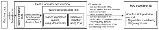
Figure 1. Remaining useful life (RUL) prediction framework for bearings. We add the section number corresponding to the explanation of each component.

In the next step, the RUL estimation module predicts the future value of the extracted health indicator based on the degradation model to estimate the RUL value in the online phase. The proposed prognostics integrate machine learning and mathematical degradation model of the time series data of the health indicator. The proposed feature importance ranking and PCA computes the health indicator based on the time series data in the online phase. We predict the time to cross the specific threshold value of the health indicator using the degradation model. An adaptive sliding window method then optimizes the model parameters of the degradation model by using the ridge regression of the time series data via the sliding window in the online phase.

4. Health Indicator Construction

In this section, we present the feature extraction and postprocessing to construct the health indicator.

4.1. Feature Extraction

Various signal processing techniques, including time domain, frequency domain, and time–frequency domain analysis, are used to construct the features. We consider not only basic statistical measures such as mean, standard deviation, and root mean square (RMS) but also the higher-order statistics such as skewness and kurtosis. All these statistics can be expected to change as a deteriorating fault signature intrudes the nominal signal [4,7]. Table 1 shows all statistical features used to build the health indicator, including 10 time domain features, 5 frequency domain features, and 12 time–frequency domain features.

Table 1. Statistical features of time domain, frequency domain, and time–frequency domain.

	Statistical Features
Time domain	mean, standard deviation, RMS, maximum-to-minimum difference, skewness,
	kurtosis, energy, signal median absolute deviation, crest factor and shape factor
Frequency domain	mean frequency, skewness, and kurtosis of the power spectrum and
	mean and standard deviation of the local maxima of the power spectrum
Time–frequency domain	mean, standard deviation, skewness and kurtosis of
	the conditional spectral moment with different orders between 2 and 4

• Time domain feature: Simple statistical features of time domain signals can serve as health indicators for predicting RUL. For instance, the average value or variance of a specific signal increases as the system performance degrades [7]. Furthermore, the higher-order statistics provide insight into system behavior through the third moment (skewness) and fourth moment (kurtosis) of the signal [4]. We use various statistical metrics of the time domain analysis including mean, standard deviation, RMS, skewness, kurtosis, maximum-to-minimum difference, sum of the square called energy, signal median absolute deviation, peak value divided by the RMS called crest factor, and RMS divided by the mean of the absolute value called shape factor.
• Frequency domain feature: Spectral analysis extracts the useful features for predicting RUL, such as bearings, gears, and engines [7,11]. The frequency domain features include power bandwidth, mean frequency, signal-to-noise ratio, and local maxima of the power spectrum of the signal. For example, the peak value of a signal spectrum or the frequency at which the peak magnitude occurs is changed as the machine degrades. The mean frequency, kurtosis, skewness of the power spectrum, and mean and standard deviation of the local maxima of the power spectrum are used as the statistical features of the frequency domain.
• Time–frequency domain feature: Another way to quantify the chaotic behavior is the time–frequency spectral properties such as spectral kurtosis and spectral entropy. Spectral kurtosis, for example, in the frequency domain, is considered a powerful method for the RUL prediction of the wind turbine [42]. Furthermore, the time–frequency moment effectively characterizes the frequency changes in time of non-stationary signals [43]. The short-time Fourier transform technique is used to capture the time-varying frequency behavior because the classical Fourier analysis fails to analyze the time-varying behavior. The conditional spectral moment of the time–frequency distribution of a signal is computed for a given sampling rate and order between 2 and 4. We then use the statistical metrics such as mean, standard deviation, skewness, and kurtosis of the conditional spectral moment with different orders.

The noise of various features substantially degrades the accuracy of the RUL prediction. Furthermore, the feature importance rank based on the monotonicity, as described below, is vulnerable to noise. We apply a moving average filter to reduce the noise effect of the features where no future feature value is used.

4.2. Feature Postprocessing

Feature postprocessing techniques construct a suitable health indicator to predict RUL built upon various statistical metrics in Table 1. For reliable RUL estimations, a health indicator requires to be observable and correlated with the system degradation process over time. The feature importance ranking and PCA identify the health indicator and threshold values for the RUL prediction.

We first select main features out of all available features in Table 1 to build a reliable RUL prediction model. A suitable condition indicator has a consistent positive or negative behavior as a system gets closer to failure. We use the monotonicity as the feature selection metric to quantify the importance of the features [42]. The monotonicity of ith feature is defined as

$$\begin{array}{c}\hfill M_i=\frac{|N_p\left({\delta }_i\right)-N_n\left({\delta }_i\right)|}{N-1}\end{array}$$

(1)

where

$$\begin{array}{c}\hfill {\delta }_i=x_i\left(t\right)-x_i(t-1),\forall t\in \{1,\dots ,N\},\end{array}$$

with $x_i\left(t\right)$ ith feature signal of sampling sequence t, N is the number of measured samples, and ${\delta }_i$ the difference of ith feature signal $x_i$ over sampling sequences. $N_p$ (respectively, $N_n$) is the number of positive (respectively, negative) values of ${\delta }_i$ for all training data. The monotonicity evaluates the feature importance score on a scale ranging from 0 to 1. A higher ranked feature tracks the degradation process more reliably and, hence, is more suitable to train the RUL prediction model. Features with large importance score are selected for feature postprocessing based on the training data in offline.

Once we identify the main features, PCA extracts the health indicator by reducing the feature dimension. PCA essentially reduces a system of a large number of features into a few principal components using a linear transformation while maintaining most of the variability from the feature set [30,31]. Note that the mean and the standard deviation obtained from training data are used to normalize the features of the entire datasets. After PCA is applied to the feature set of the training data, we select the specific principal component out of multiple principal components as the health indicator if it increases as the machine degrades.

5. Parameter Estimation of Degradation Model

We estimate the RUL value by developing a degradation model of the time series health indicator. The degradation model identifies a dynamic model that describes the failure process of the system behavior. It predicts the health indicator and the time to cross a specific threshold of the health indicator as the failure indicator.

We assume that the health indicator $h\left(t_i\right)$ of bearings is observed at discrete times $t_1,t_2,\dots ,$ where $t_i\ge 0$. Exponential degradation models are useful when the machine component experiences cumulative degradation [8]. Besides, the linear degradation model is another useful one if the observed system does not have cumulative degradation processes [33,44]. Hence, the considered degradation model combines the exponential model and the linear model as follows:

$$\begin{array}{cc}\hfill {\widehat{h}}_w\left(t_i\right)& =\varphi +{\beta }_w{t}_i+{\alpha }_{w}exp\left(t_i\right)\hfill \end{array}$$

(2)

where $\varphi ,{\beta }_w$ and ${\alpha }_w$ are the updated parameters dependent on the health indicator over the sliding window. Compared to the existing exponential degradation model [8], the exponential part of Equation (2) reduces the flexibility of the degradation model. The sliding window method adapts the local model parameters of the time series data to compensate for the fundamental limits of the analytical degradation model. We evaluate the RUL prediction accuracy and robustness of the proposed scheme in Section 7.

The adaptive sliding window method relies on ridge regression to balance training accuracy and generalization accuracy. We formulate the ridge regression problem by combining the prediction error term and the regulation term with different weights on model parameters $\mathbf{x}={\left[\varphi ,{\alpha }_w,{\beta }_w\right]}^{\top }$ to avoid the overfitting and reduce the critical effect of the exponential term of Equation (2). The parameter optimization problem of the adaptive sliding window method is

$$\begin{array}{c}\hfill {\min }_{\mathbf{x}}\sum _{j=i-s+1}^i{(h\left(t_j\right)-{\widehat{h}}_w\left(t_j\right))}^2+{\mathbf{x}}^{\top }\mathbf{W}\mathbf{x}\forall t_i\in 1,\dots ,N\end{array}$$

(3)

where the first term is the mean square error between measured health indicators $h\left(t_j\right)$ and estimated health indicators ${\widehat{h}}_w\left(t_j\right)$ with sliding length s and the second term is the weighted regularization term with diagonal matrix $\mathbf{W}\in {\mathbb{R}}^{3\times 3}$. Each element of the diagonal matrix $\mathbf{W}$ corresponds to the weight of the decision variable of $\mathbf{x}$.

Since the objective function is a regularized quadratic cost function, we rewrite it as the matrix form

$$\begin{array}{c}\hfill J\left(\mathbf{x}\right)={(\mathbf{h}-\mathbf{A}\mathbf{x})}^{\top }(\mathbf{h}-\mathbf{A}\mathbf{x})+{\mathbf{x}}^{\top }\mathbf{W}\mathbf{x},\end{array}$$

(4)

where

$$\begin{array}{c}\hfill \mathbf{A}=\left[\begin{array}{ccc}1& exp\left(t_{i-s+1}\right)& t_{i-s+1}\\ 1& exp\left(t_{i-s+2}\right)& t_{i-s+2}\\ ⋮& ⋮& ⋮\\ 1& exp\left(t_i\right)& t_i\end{array}\right]\in {\mathbb{R}}^{s\times 3},\end{array}$$

and

$$\begin{array}{c}\hfill \mathbf{h}=\left[\begin{array}{c}h\left(t_{i-s+1}\right)\\ h\left(t_{i-s+2}\right)\\ ⋮\\ h\left(t_i\right)\end{array}\right]\in {\mathbb{R}}^s.\end{array}$$

The optimal solution is

$$\begin{array}{c}\hfill {\mathbf{x}}^{*}={({\mathbf{A}}^{\top }\mathbf{A}+\mathbf{W})}^{-1}{\mathbf{A}}^{\top }\mathbf{h}.\end{array}$$

(5)

Determining the optimal length of the sliding window is a complex task since it requires to take into account the reduction of the noise effect and the fault detection delay. The sliding window length is set to 30 s based on the estimation accuracy of the health indicator of the training sets for different sliding window lengths from 10 to 102 s.

6. Evaluation Setup

In this section, we describe the benchmark dataset of the mechanical bearings and the existing Bayesian approach that we used to compare our proposed method.

6.1. PHM Challenge Problem

PRONOSTIA is an experimental platform developed by the FEMTO-ST institute to evaluate and validate various fault detection and diagnostic algorithms of ball bearings [45]. The platform consists of three parts, namely rotating part, a measurement part, and a degradation generation part. It provides experimental measurements of accelerated degradation of mechanical bearings with constant or variable rotating speed and load force. Dedicated sensors measure the vibration and temperature of the platform. Two miniature accelerometers are installed orthogonally on the external race of the bearing to monitor the vertical and horizontal vibrations. The temperature sensor is located near the external ring of the bearing. These measurements are used to extract the health indicator of ball bearings.

PRONOSTIA platform provides various run-to failure experimental data since it enables the experimental degradation within a few hours. Seventeen experimental data cases are generated under three different operating conditions of rotating speed and load force, as summarized in Table 2. The experimental data includes 6 run-to-failure training sets and 11 remaining test sets to build RUL estimation models and evaluate the accuracy. Note that we use the notation $\mathtt{i}\_\mathtt{j}$ to denote jth dataset of operating condition i where $i\in \{\mathtt{A},\mathtt{B},\mathtt{C}\}$. The vibration and temperature signals are recorded with specific sampling frequencies of 25.6 kHz and 10 Hz, respectively. Each experiment is terminated if the vibration signal reaches 20 g to prevent testbed damages. Hence, RUL is defined as time to accelerometer exceeding 20 g. Note that the RUL prediction method is only able to use the measurements of ball bearings since the detailed information of the degradation process is not provided.

Table 2. Specifications of the experimental data.

	Operating Condition A	Operating Condition B	Operating Condition C
Load force (N)	4000	4200	5000
Speed (rpm)	1800	1650	1500
Training dataset	Bearing $\mathtt{A}\_\mathtt{1}$, Bearing $\mathtt{A}\_\mathtt{2}$	Bearing $\mathtt{B}\_\mathtt{1}$, Bearing $\mathtt{B}\_\mathtt{2}$	Bearing $\mathtt{C}\_\mathtt{1}$, Bearing $\mathtt{C}\_\mathtt{2}$
Testing dataset	Bearing $\mathtt{A}\_\mathtt{3}$, Bearing $\mathtt{A}\_\mathtt{4}$,	Bearing $\mathtt{B}\_\mathtt{3}$, Bearing $\mathtt{B}\_\mathtt{4}$,	Bearing $\mathtt{C}\_\mathtt{3}$
	Bearing $\mathtt{A}\_\mathtt{5}$, Bearing $\mathtt{A}\_\mathtt{6}$,	Bearing $\mathtt{B}\_\mathtt{5}$, Bearing $\mathtt{B}\_\mathtt{6}$,
	Bearing $\mathtt{A}\_\mathtt{7}$	Bearing $\mathtt{B}\_\mathtt{7}$

Figure 2 depicts a horizontal vibration raw signal of various cases Bearing $\mathtt{A}\_\mathtt{1}$, Bearing $\mathtt{A}\_\mathtt{2}$, Bearing $\mathtt{B}\_\mathtt{1}$, Bearing $\mathtt{B}\_\mathtt{2}$, Bearing $\mathtt{C}\_\mathtt{1}$, Bearing $\mathtt{C}\_\mathtt{2}$ obtained during a whole experiment. The degradation processes of bearings have considerably different behaviors with various experimental duration (1–7 h). Efficient estimator design is challenging due to a small amount of training data with a high variation of the life duration of all bearings. As the machine progressively approaches to failure, the vibration signal impulsiveness increases. While the acceleration of operating condition $\mathtt{A}$ is slowly growing over time, it is suddenly raised under condition $\mathtt{C}$. Furthermore, we observe significantly different behaviors even under the same operating condition, such as cases Bearing $\mathtt{A}\_\mathtt{1}$ and Bearing $\mathtt{A}\_\mathtt{2}$. The raw vibration signals do not have a clear correlation with various operating conditions.

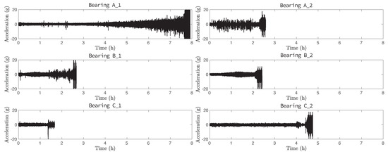
Figure 2. Horizontal vibration raw signal of training cases Bearing $\mathtt{A}\_\mathtt{1}$, Bearing $\mathtt{A}\_\mathtt{2}$, Bearing $\mathtt{B}\_\mathtt{1}$, Bearing $\mathtt{B}\_\mathtt{2}$, Bearing $\mathtt{C}\_\mathtt{1}$, and Bearing $\mathtt{C}\_\mathtt{2}$.

In a typical framework, the machine learning trains a regression model based on the data of some bearings and uses it to predict the RUL value of the other bearings. However, even if we obtain the measurements of the same type of bearing under the identical operating condition, their probabilistic density functions are considerably different due to various uncertainties. Hence, most existing machine learning algorithms result in a substantial performance loss because of the violation of the i.i.d. condition even with the same operating condition. While many mathematical models using frequency domain features efficiently detect the faults of the inner and outer races of ball bearings, they are hard to apply in practice due to the extraction difficulty of the frequency features under complex interactions [45]. Moreover, the statistical features of various cases tend to have different noise levels depending on the degradation process. Hence, a single regression model trained on limited data is difficult to generalize for other cases.

6.2. Bayesian Approach

The Bayesian method estimates the parameters of the degradation model based on its prior probability distribution and current measurements [8]. Two degradation models are considered, namely exponential and linear degradation models, to predict RUL of bearings using experimental data. The discrete-time exponential degradation model is defined as

$$\begin{array}{cc}\hfill {\widehat{h}}_e\left(t_i\right)& ={\varphi }_e+{\alpha }_{e}exp\left({\theta }_e{t}_i+ϵ-\frac{{\sigma }^2}{2}\right)\hfill \end{array}$$

(6)

where the predicted health indicator ${\widehat{h}}_e\left(t_i\right)$ is a function of time, ${\varphi }_e$ is the constant intercept, ${\alpha }_e$ and ${\theta }_e$ are stochastic parameters deciding the slope of the model, and $ϵ$ is a normally distributed random error with $N(0,{\sigma }^2)$. In addition, ${\alpha }_e$ is lognormal-distributed and ${\theta }_e$ is Gaussian-distributed [8].

We also define the discrete-time linear degradation model as

$$\begin{array}{cc}\hfill {\widehat{h}}_l\left(t_i\right)& ={\varphi }_l+{\beta }_l{t}_i+ϵ\hfill \end{array}$$

(7)

where ${\varphi }_l$ is the model intercept, ${\beta }_l$ is a Gaussian-distributed random parameter determining the slope, and $ϵ$ is a normally distributed random noise with $N(0,{\sigma }^2)$.

At each time step $t_i$, Bayesian estimator updates the distribution of model parameters of Equations (6) and (7) based on the previous knowledge of the model and the latest observation of $h\left(t_i\right)$ as the basis for the RUL prediction. We initially set the slope of the exponential degradation model based on the historical training data. If historical data are not available, the prior of the slope parameters are randomly selected with large variances to rely more on the observed data during the initial setup.

Since the performance of Bayesian methods considerably depends on the models and the data, as discussed below, we also propose an adaptive Bayesian method to choose one of the models between the exponential degradation model and the linear degradation model based on the residual error between the proposed model and measured health indicator.

7. Performance Evaluation

In this section, we evaluate the performance of the RUL estimation obtained by the adaptive sliding window method and the Bayesian method for various experimental data. We first discuss the feature extraction and postprocessing and then evaluate the accuracy of the RUL prediction.

7.1. Feature Extraction and Postprocessing

Figure 3 shows the power spectrum as a function of time and frequency of Bearing $\mathtt{B}\_\mathtt{2}$. The colorbar indicates the fault severity normalized to 1, dependent on the RUL value of the experiment. As the machine progressively approaches to failure, the power spectrum around 13 kHz gradually increases. Hence, the statistical features of the power spectrum are potential indicators of degraded bearings.

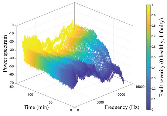
Figure 3. Power spectrum over time and frequency of Bearing $\mathtt{B}\_\mathtt{2}$.

Various statistical features of time domain, frequency domain, and time–frequency domain signals, as listed in Table 1, are used to construct the health indicator. We only select main features with monotonicity greater than $0.4$ as the input to PCA for feature fusion by considering all training sets. Note that we only use the training data to select the main features for the health indicator. These features are standard deviation, RMS, energy, median absolute deviation of the time domain, and mean and standard deviation of the conditional spectral moment with orders 2 and 3 in the time–frequency domain. Besides, the mean, skewness, kurtosis, and standard deviation of the local maxima of the power spectrum are selected in the frequency domain. One interesting finding is that the operating condition is not a critical factor in the feature importance ranking using the monotonicity.

Once the main features are selected using the monotonicity rank, PCA is applied to construct the health indicator by reducing the dimension of feature spaces. Before performing PCA, the mean and standard deviation of training data normalize the whole data. Figure 4 shows the projected data onto the first two principal components obtained by PCA of Bearing $\mathtt{A}\_\mathtt{2}$. We clearly observe that the first principal component increases as the machine gets closer to failure. We use the first principal component as the health indicator for the RUL prediction.

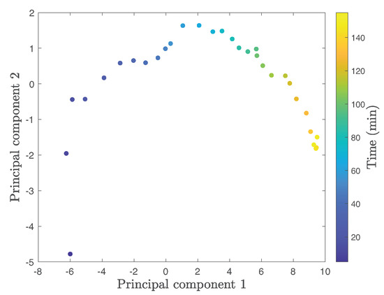
Figure 4. Two principal components of Bearing $\mathtt{A}\_\mathtt{2}$.

Figure 5 presents the health indicators of various training cases Bearing $\mathtt{A}\_\mathtt{1}$, Bearing $\mathtt{A}\_\mathtt{2}$, Bearing $\mathtt{B}\_\mathtt{1}$, Bearing $\mathtt{B}\_\mathtt{2}$, Bearing $\mathtt{C}\_\mathtt{1}$, Bearing $\mathtt{C}\_\mathtt{2}$ as a function of experimental time. We observe that the health indicator monotonically increases under various operating conditions with different cases. While each case shows significantly different health indicator at the initial state, all cases converge to a similar health indicator value as the machine approaches failure. Based on these observations, we set the threshold as 9, around 90% of the maximum value of the health indicators of the training data, to reduce the delay effect of smoothing.

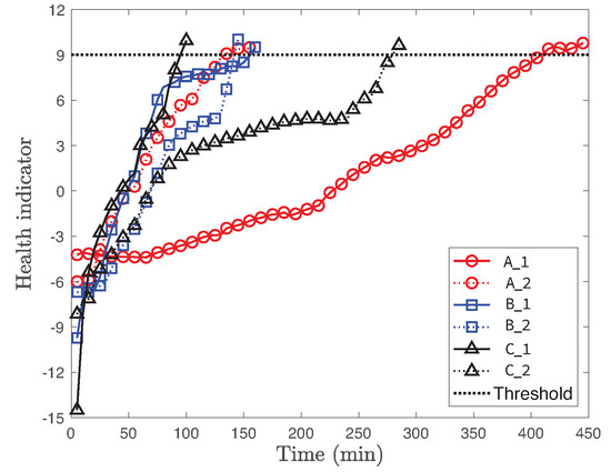
Figure 5. Health indicator of training cases Bearing $\mathtt{A}\_\mathtt{1}$, Bearing $\mathtt{A}\_\mathtt{2}$, Bearing $\mathtt{B}\_\mathtt{1}$, Bearing $\mathtt{B}\_\mathtt{2}$, Bearing $\mathtt{C}\_\mathtt{1}$, Bearing $\mathtt{C}\_\mathtt{2}$ as a function of experimental time.

Another interesting observation is that the operating condition is not a dominant factor to characterize the health indicator. For instance, two different cases Bearing $\mathtt{A}\_\mathtt{1}$ and Bearing $\mathtt{A}\_\mathtt{2}$ of same operating condition are considerably different. On the other hand, the health indicators of both Bearing $\mathtt{B}\_\mathtt{2}$ and Bearing $\mathtt{C}\_\mathtt{2}$ are similar and rise rapidly when the bearing is closer to the end, even if they have different operating conditions. Hence, it clearly shows that the health indicator significantly varies due to the complex interactions of machine components and high uncertainty.

7.2. RUL Evaluation

Figure 6 presents the health indicator and RUL of true measurements, adaptive sliding window method, and Bayesian methods using the exponential and the linear degradation models of Bearing $\mathtt{B}\_\mathtt{6}$ as a function of experimental time. In Figure 6b, we also show the $\alpha$ bound of the true RUL where $\alpha$ is set to 20%. Figure 6a depicts that the health indicator of Bearing $\mathtt{B}\_\mathtt{6}$ gradually increases as a function of experimental time. Both the adaptive sliding window method and the Bayesian method using the linear degradation model follow the true health indicator. On the contrary, the Bayesian method using the exponential degradation model fails to estimate the health indicator. The main reason is the fundamental model limits of the exponential degradation model with respect to the slowly degraded health indicator of Bearing $\mathtt{B}\_\mathtt{6}$.

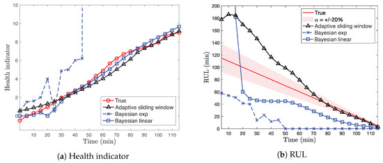
Figure 6. Health indicators and RUL of true measurements, adaptive sliding window method, and Bayesian methods using the exponential and the linear degradation models of Bearing $\mathtt{B}\_\mathtt{6}$.

By comparing Figure 6a,b, we observe that predicting the health indicator is not enough to estimate the RUL value due to the complex interaction between machine components with high uncertainty during whole experimental times. In fact, some experimental cases show sudden performance degradation when it gets closer to failure, as shown in Figure 2. Hence, it is infeasible to provide an accurate estimation of RUL at the beginning of the experimental operations. However, the adaptive sliding window method still provides the reasonable estimation of RUL within the $\alpha$-bound of the true RUL for Bearing $\mathtt{B}\_\mathtt{6}$ as it is closer to failure, as shown in Figure 6b. Both Bayesian methods using different models generally provide the conservative RUL prediction during the experimental time. Although the Bayesian method using the exponential degradation model does not provide the reasonable RUL estimation for Bearing $\mathtt{B}\_\mathtt{6}$ due to the fundamental model limit, the performance of different methods considerably depends on the degradation trends of the real health indicator of each case, as we show below.

We use the error ratio metric to evaluate the RUL prediction of different methods. Let us denote $y_i$ and $\widehat{y_i}$ as the actual RUL to be predicted and the estimated RUL of ith dataset, respectively. The error ratio of of ith dataset is defined by

$$\begin{array}{c}\hfill R_i=\frac{y_i-\widehat{y_i}}{y_i}.\end{array}$$

(8)

The effects of RUL underestimation and overestimation are not the same in practice. While early predictions of RUL, $R_i>0$, are considered as the reasonable estimation with the deduction to early removal, the RUL estimation that exceeded actual RUL, $R_i<0$, incurs more severe consequences.

Based on this observation, the IEEE PHM Data Challenge defines a scoring function

$$\begin{array}{cc}\hfill \mathrm{Score}& =\frac{1}{11}\sum _{i=1}^{11}{A}_i\hfill \end{array}$$

(9)

where

$$\begin{array}{c}\hfill A_i=\left\{\begin{array}{cc}exp(-\ln \left(0.5\right)(P_i/5))\hfill & P_i\le 0\hfill \\ exp(+\ln \left(0.5\right)(P_i/20))\hfill & P_i>0\hfill \end{array}\right.\end{array}$$

(10)

and $P_i$ denotes the percent error equal to Equation (8) multiplied by 100 for ith testing set [45].

The accuracy of the RUL prediction becomes more critical as the machine approaches to failure over time. To analyze the RUL prediction performance over time, we evaluate the error ratio of different solutions in each interval of 10% based on the time sequences to the whole experimental time. In this evaluation, we show the RUL prediction between 60% and 100% of the experimental time of each case since the first 40% of data are not a critical factor for the practical purpose of the maintenance. For instance, the error ratio between $90\%$ and $100\%$ of the experimental time means the average error ratio of the last 10% of the experimental data.

Figure 7 presents the normalized histogram of error ratios in each interval of 10% from 60% to 100% of the experimental time using different approaches for all cases. The adaptive sliding window method, Bayesian methods using the exponential and the linear degradation models, and adaptive Bayesian method provide considerably different error ratios of the RUL estimation as a function of time. One interesting observation is that the overall error ratio using Bayesian methods is gradually shifted from the positive error ratio to 0 as a function of time. It means that these methods provide a better underestimation of RUL prediction as the machine approaches to failure. While the histogram of the adaptive Bayesian method is similar to the one of the exponential degradation model for the error ratio around 0, the large error ratio greater than $0.6$ is reduced thanks to the linear degradation model. The RUL prediction error ratio of the adaptive Bayesian method is improved compared to the ones using either exponential degradation model or linear degradation model.

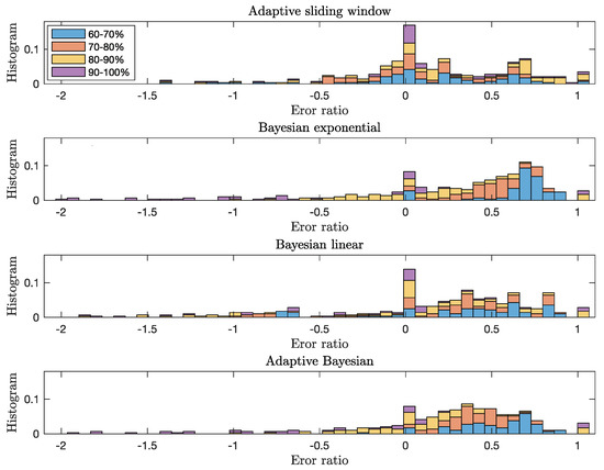
Figure 7. Normalized error ratio histogram of the RUL prediction of adaptive sliding window method, Bayesian methods using the exponential and the linear degradation models, and adaptive Bayesian method as a function of the experimental time. We split the error ratio of different solutions in each interval of 10% based on the time sequences with respect to the entire experimental time to analyze the performance of the RUL prediction over time.

While the error ratio using Bayesian methods is spread around $0.5$, the one using the adaptive sliding window method is concentrated around 0. We observe that most absolute error ratios between 90% and 100% of the experimental time are less than $0.1$ or larger than 1 for all cases. The main reason for the high negative or positive ratio is the small value of the true RUL of Equation (8) as the machine approaches to the end.

The score of the adaptive sliding window method is $0.6028$, greater than that of the adaptive Bayesian method ($0.4605$). Note that the score values are $0.2554$ and $0.3827$ for Bayesian methods using the exponential and the linear degradation models, respectively. The score of the recently developed multiscale CNN method [10] is $0.3624$, while the adaptive sliding window method gives $0.3117$ for five test sets of the operating condition $\mathtt{A}$. Note that Zhu et al. [10] only provided the score value of the operating condition $\mathtt{A}$. However, our proposed scheme significantly reduces the computation complexity while guaranteeing the robustness against the possible uncertainty. Note that DL models are vulnerable to input uncertainties or adversarial attacks [14,15].

Mean absolute error (MAE) and mean absolute percentage error (MAPE) are used to evaluate prediction performance with the following formula:

$$\begin{array}{cc}\hfill \mathrm{MAE}& =\frac{1}{N}\sum _{i=1}^N|y_i-{\widehat{y}}_i|,\hfill \end{array}$$

(11)

$$\begin{array}{cc}\hfill \mathrm{MAPE}& =\frac{1}{N}\sum _{i=1}^N\left|\frac{y-{\widehat{y}}_i}{y_i}\right|,\hfill \end{array}$$

(12)

where N is the number of samples. Note that we do not show the root-mean-squared error since it has a similar trend with the MAE results. Figure 8 shows MAE and MAPE between true RUL value and predicted RUL obtained by adaptive sliding window method, Bayesian methods using the exponential and the linear degradation models, and adaptive Bayesian method for all cases. We observe that various approaches have considerably different MAEs of the RUL estimation dependent on cases. Since we do not reuse any specific model parameters of the training sets to evaluate the testing sets, the performance of the training sets does not necessarily better than the ones of testing sets. The adaptive sliding window method provides the smallest MAE for 12 cases out of 17 cases. It outperforms all cases with operating condition $\mathtt{C}$ and $\mathtt{B}$ except the case of Bearing $\mathtt{B}\_\mathtt{7}$. The RUL MAE using the adaptive sliding window method is only worse than other approaches for Bearing $\mathtt{A}\_\mathtt{3}$, Bearing $\mathtt{A}\_\mathtt{4}$, Bearing $\mathtt{A}\_\mathtt{5}$, Bearing $\mathtt{A}\_\mathtt{7}$, Bearing $\mathtt{B}\_\mathtt{7}$. This is the main reason for the high positive or negative error ratio of the adaptive sliding window method in Figure 7.

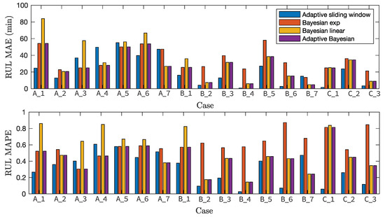
Figure 8. RUL MAE and MAPE obtained by adaptive sliding window method, Bayesian methods using the exponential and the linear degradation models, and adaptive Bayesian method for all cases.

The adaptive Bayesian method outperforms the adaptive sliding window method for five cases out of 17 cases. These five cases consist of four cases with condition $\mathtt{A}$ and a single case with condition $\mathtt{B}$. In these five cases, the Bayesian estimator using the exponential degradation model performs better than the ones using the linear degradation model for three cases with condition $\mathtt{A}$. It is an interesting observation since the linear degradation model outperforms the exponential one for 10 cases out of 17 cases. While the adaptive sliding window method generally outperforms the Bayesian method using the linear degradation model, it cannot fully replace the Bayesian method using the exponential degradation model. The main reason is the fundamental model limits of the degradation model of Equation (2) for specific cases of Bearing $\mathtt{A}\_\mathtt{3}$, Bearing $\mathtt{A}\_\mathtt{4}$, Bearing $\mathtt{A}\_\mathtt{5}$.

The overall trends of MAPE results are similar to those of the MAE results. The average value of all MAPE values of the adaptive sliding window is $0.3087$, lower than that of the adaptive Bayesian method ($0.4343$). Note that the average values of all MAPEs are $0.6056$ and $0.5229$ for Bayesian methods using the exponential and the linear degradation models, respectively.

8. Conclusions

In this paper, we propose the RUL prediction method of mechanical bearings combining model-based and data-driven approaches. The adaptive sliding window method optimizes the local model parameters of the degradation model based on the ridge regression of the time series health indicator to estimate the RUL value. We compare the performance of the proposed scheme to existing Bayesian approaches for predicting the RUL value of the experimental data of the PHM data challenge problem. The adaptive sliding window method provides the smallest mean absolute error for 12 cases out of 17 cases. Furthermore, it achieves around 28% improvement in terms of mean absolute error and mean absolute percentage error with respect to the ones using Bayesian approaches. One interesting finding is that predicting the health indicator is not enough to estimate the RUL value due to the complex interaction between machine components with high uncertainty during the whole experimental times. Even though some existing Bayesian approaches estimate the health indicator well, the performance considerably depends on the degradation model. The adaptive sliding window approach provides significant performance improvement and robustness against the possible errors of the degradation model with respect to the ones using Bayesian approaches. The robustness to the model error is crucial to deploy the actual algorithm in industrial systems since it is not feasible to derive the universal degradation model even for the same bearing.

In practical industrial systems, a full coverage of representative data of all possible failures and their combinations is typically not available, while it is a critical factor for the accurate RUL estimation. For instance, our degradation model is not general enough to capture various behaviors due to many uncertainties in practice. The RUL estimation is essentially the behavior forecasting problem of the time series data using the sparse and delayed measurement with high noise and uncertainty. Furthermore, each failure mode typically has long-term dependencies along with short-term ones of time series data. Future research will focus on bridging the gap between the traditional knowledge of mathematical models and the deep learning techniques to estimate RUL using the time series data.

References

- Lu, B.; Durocher, D.B.; Stemper, P. Predictive maintenance techniques. IEEE Ind. Appl. Mag. 2009, 15, 52–60. [Google Scholar] [CrossRef]
- Vichare, N.M.; Pecht, M.G. Prognostics and health management of electronics. IEEE Trans. Components Packag. Technol. 2006, 29, 222–229. [Google Scholar] [CrossRef]
- Jasiulewicz-Kaczmarek, M.; Legutko, S.; Piotr, K. Maintenance 4.0 technologies—New opportunities for sustainability driven maintenance. Manag. Prod. Eng. Rev. 2020, 11, 74–87. [Google Scholar]
- Jardine, A.K.; Lin, D.; Banjevic, D. A review on machinery diagnostics and prognostics implementing condition-based maintenance. Mech. Syst. Signal Process. 2006, 20, 1483–1510. [Google Scholar] [CrossRef]
- Heng, A.; Tan, A.C.; Mathew, J.; Montgomery, N.; Banjevic, D.; Jardine, A.K. Intelligent condition-based prediction of machinery reliability. Mech. Syst. Signal Process. 2009, 23, 1600–1614. [Google Scholar] [CrossRef]
- Jasiulewicz-Kaczmarek, M.; Gola, A. Maintenance 4.0 Technologies for Sustainable Manufacturing—An Overview. IFAC PapersOnLine 2019, 52, 91–96. [Google Scholar] [CrossRef]
- Nandi, S.; Toliyat, H.A.; Li, X. Condition monitoring and fault diagnosis of electrical motors—A review. IEEE Trans. Energy Convers. 2005, 20, 719–729. [Google Scholar] [CrossRef]
- Gebraeel, N. Sensory-updated residual life distributions for components with exponential degradation patterns. IEEE Trans. Autom. Sci. Eng. 2006, 3, 382–393. [Google Scholar] [CrossRef]
- Jin, X.; Zhao, M.; Chow, T.W.S.; Pecht, M. Motor bearing fault diagnosis using trace ratio linear discriminant analysis. IEEE Trans. Ind. Electron. 2014, 61, 2441–2451. [Google Scholar] [CrossRef]
- Zhu, J.; Chen, N.; Peng, W. Estimation of Bearing Remaining Useful Life Based on Multiscale Convolutional Neural Network. IEEE Trans. Ind. Electron. 2019, 66, 3208–3216. [Google Scholar] [CrossRef]
- Heng, A.; Zhang, S.; Tan, A.C.; Mathew, J. Rotating machinery prognostics: State of the art, challenges and opportunities. Mech. Syst. Signal Process. 2009, 23, 724–739. [Google Scholar] [CrossRef]
- Park, P.; Marco, P.D.; Shin, H.; Bang, J. Fault Detection and Diagnosis Using Combined Autoencoder and Long Short-Term Memory Network. Sensors 2019, 19, 4612. [Google Scholar] [CrossRef]
- Moosavi-Dezfooli, S.; Fawzi, A.; Fawzi, O.; Frossard, P. Universal adversarial perturbations. In Proceedings of the IEEE Conference on Computer Vision and Pattern Recognition, Honolulu, HI, USA, 21–26 July 2017; pp. 86–94. [Google Scholar]
- Szegedy, C.; Zaremba, W.; Sutskever, I.; Bruna, J.; Erhan, D.; Goodfellow, I.; Fergus, R. Intriguing properties of neural networks. In Proceedings of the International Conference on Learning Representations, Banff, AB, Canada, 14–16 April 2014; pp. 1–10. [Google Scholar]
- Zheng, S.; Song, Y.; Leung, T.; Goodfellow, I. Improving the robustness of deep neural networks via stability training. In Proceedings of the IEEE Conference on Computer Vision and Pattern Recognition, Las Vegas, NV, USA, 27–30 June 2016; pp. 4480–4488. [Google Scholar]
- Bojarski, M.; Testa, D.D.; Dworakowski, D.; Firner, B.; Flepp, B.; Goyal, P.; Jackel, L.D.; Monfort, M.; Muller, U.; Zhang, J.; et al. End to end learning for self-driving cars. arXiv 2018, arXiv:1604.07316. [Google Scholar]
- Julian, K.D.; Lopez, J.; Brush, J.S.; Owen, M.P.; Kochenderfer, M.J. Policy compression for aircraft collision avoidance systems. In Proceedings of the IEEE/AIAA 35th Digital Avionics Systems Conference, Sacramento, CA, USA, 25–30 September 2016; pp. 1–10. [Google Scholar]
- Xiang, W.; Musau, P.; Wild, A.A.; Lopez, D.M.; Hamilton, N.; Yang, X.; Rosenfeld, J.A.; Johnson, T.T. Verification for machine learning, autonomy, and neural networks survey. arXiv 2018, arXiv:1810.01989. [Google Scholar]
- Botvinick, M.; Ritter, S.; Wang, J.X.; Kurth-Nelson, Z.; Blundell, C.; Hassabis, D. Reinforcement learning, fast and slow. Trends Cogn. Sci. 2019, 23, 408–422. [Google Scholar] [CrossRef]
- Wang, Y.; Ma, E.W.M.; Chow, T.W.S.; Tsui, K. A two-step parametric method for failure prediction in hard disk drives. IEEE Trans. Ind. Inform. 2014, 10, 419–430. [Google Scholar] [CrossRef]
- Park, P.; Ergen, S.C.; Fischione, C.; Lu, C.; Johansson, K.H. Wireless network design for control systems: A survey. IEEE Commun. Surv. Tutor. 2018, 20, 978–1013. [Google Scholar] [CrossRef]
- Lei, Y.; Li, N.; Guo, L.; Li, N.; Yan, T.; Lin, J. Machinery health prognostics: A systematic review from data acquisition to RUL prediction. Mech. Syst. Signal Process. 2018, 104, 799–834. [Google Scholar] [CrossRef]
- Cubillo, A.; Perinpanayagam, S.; Esperon-Miguez, M. A review of physics-based models in prognostics: Application to gears and bearings of rotating machinery. Adv. Mech. Eng. 2016, 8. [Google Scholar] [CrossRef]
- Si, X.-S.; Wang, W.; Hu, C.-H.; Zhou, D.-H. Remaining useful life estimation a review on the statistical data driven approaches. Eur. J. Oper. Res. 2011, 213, 1–14. [Google Scholar] [CrossRef]
- Tian, Z.; Liao, H. Condition based maintenance optimization for multi-component systems using proportional hazards model. Reliab. Eng. Syst. Saf. 2011, 96, 581–589. [Google Scholar] [CrossRef]
- Qian, Y.; Yan, R.; Hu, S. Bearing Degradation Evaluation Using Recurrence Quantification Analysis and Kalman Filter. IEEE Trans. Instrum. Meas. 2014, 63, 2599–2610. [Google Scholar] [CrossRef]
- Kozłowski, E.; Mazurkiewicz, D.; Zabinski, T.; Prucnal, S.; Sep, J. Machining sensor data management for operation-level predictive model. Expert Syst. Appl. 2020, 159, 113600. [Google Scholar] [CrossRef]
- Soualhi, A.; Medjaher, K.; Zerhouni, N. Bearing Health Monitoring Based on HilbertHuang Transform, Support Vector Machine, and Regression. IEEE Trans. Instrum. Meas. 2015, 64, 52–62. [Google Scholar] [CrossRef]
- Benkedjouh, T.; Medjaher, K.; Zerhouni, N.; Rechak, S. Fault prognostic of bearings by using support vector data description. In Proceedings of the IEEE Conference on Prognostics and Health Management, Denver, CO, USA, 18–21 June 2012; pp. 1–7. [Google Scholar]
- Sutrisno, E.; Oh, H.; Vasan, A.S.S.; Pecht, M. Estimation of remaining useful life of ball bearings using data driven methodologies. In Proceedings of the IEEE Conference on Prognostics and Health Management, Denver, CO, USA, 18–21 June 2012; pp. 1–7. [Google Scholar]
- Wang, P.; Youn, B.D.; Hu, C. A generic probabilistic framework for structural health prognostics and uncertainty management. Mech. Syst. Signal Process. 2012, 28, 622–637. [Google Scholar] [CrossRef]
- Liu, Z.; Zuo, M.J.; Qin, Y. Remaining useful life prediction of rolling element bearings based on health state assessment. J. Mech. Eng. Sci. 2016, 230, 314–330. [Google Scholar] [CrossRef]
- Mosallam, A.; Medjaher, K.; Zerhouni, N. Data-driven prognostic method based on Bayesian approaches for direct remaining useful life prediction. J. Intell. Manuf. 2016, 27, 1037–1048. [Google Scholar] [CrossRef]
- Yu, Y.; Hu, C.; Si, X.; Zhang, J. Degradation data-driven remaining useful life estimation in the absence of prior degradation knowledge. J. Control Sci. Eng. 2017, 2017, 4375690. [Google Scholar]
- Liu, R.; Meng, G.; Yang, B.; Sun, C.; Chen, X. Dislocated time series convolutional neural architecture: An intelligent fault diagnosis approach for electric machine. IEEE Trans. Ind. Inform. 2017, 13, 1310–1320. [Google Scholar] [CrossRef]
- Jing, L.; Wang, T.; Zhao, M.; Wang, P. An adaptive multi-sensor data fusion method based on deep convolutional neural networks for fault diagnosis of planetary gearbox. Sensors 2017, 17, 414. [Google Scholar] [CrossRef]
- Ince, T.; Kiranyaz, S.; Eren, L.; Askar, M.; Gabbouj, M. Real-time motor fault detection by 1-d convolutional neural networks. IEEE Trans. Ind. Electron. 2016, 63, 7067–7075. [Google Scholar] [CrossRef]
- Guo, L.; Lei, Y.; Li, N.; Yan, T.; Li, N. Machinery health indicator construction based on convolutional neural networks considering trend burr. Neurocomputing 2018, 292, 142–150. [Google Scholar] [CrossRef]
- Ren, L.; Cui, J.; Sun, Y.; Cheng, X. Multi-bearing remaining useful life collaborative prediction: A deep learning approach. J. Manuf. Syst. 2017, 43, 248–256. [Google Scholar] [CrossRef]
- Zhao, R.; Yan, R.; Wang, J.; Mao, K. Learning to monitor machine health with convolutional Bi-directional LSTM networks. Sensors 2017, 17, 273. [Google Scholar] [CrossRef]
- Goodfellow, I.; Bengio, Y.; Courville, A. Deep Learning; MIT Press: Cambridge, MA, USA, 2016. [Google Scholar]
- Saidi, L.; Ali, J.B.; Bechhoefer, E.; Benbouzid, M. Wind turbine high-speed shaft bearings health prognosis through a spectral Kurtosis- derived indices and SVR. Appl. Acoust. 2017, 120, 1–8. [Google Scholar] [CrossRef]
- Loughlin, P.; Cakrak, F.; Cohen, L. Conditional moments analysis of transients with application to helicopter fault data. Mech. Syst. Signal Process. 2000, 14, 511–522. [Google Scholar] [CrossRef]
- Chakraborty, S.; Gebraeel, N.; Lawley, M.; Wan, H. Residual-life estimation for components with non-symmetric priors. IIE Trans. 2009, 41, 372–387. [Google Scholar] [CrossRef]
- Nectoux, P.; Gouriveau, R.; Medjaher, K.; Ramasso, E.; Chebel-Morello, B.; Zerhouni, N.; Varnier, C. PRONOSTIA: An experimental platform for bearings accelerated degradation tests. In Proceedings of the IEEE International Conference on Prognostics and Health Management, Denver, CO, USA, 18–21 June 2012; pp. 1–8. [Google Scholar]
Publisher’s Note: MDPI stays neutral with regard to jurisdictional claims in published maps and institutional affiliations. |
© 2020 by the authors. Licensee MDPI, Basel, Switzerland. This article is an open access article distributed under the terms and conditions of the Creative Commons Attribution (CC BY) license (http://creativecommons.org/licenses/by/4.0/).