1. Introduction
Automated Driving Systems (ADSs) have the potential to reduce the number of accidents, lower emissions, transport the physically-impaired, and reduce the driver’s workload [
1]. Based on the Society of Automotive Engineers (SAE), ADS describes the variety of commonly used terms in intelligent transportation field, e.g.,: autonomous, self-driving, driverless, etc. [
2].
Most ADSs break down several tasks of automated driving and, by utilizing an array of sensors and algorithms, they can be solved accordingly. Path planning is one of the essential requirements for all ADSs. The path planning stage of a vehicle requires it to obey traffic rules within road networks while a robot has no specific requirements to follow [
3].
The scenario of path planning involves planning in known and unknown scenarios. Further enhancement involves planning for static and dynamic obstacles. Various perception sensing devices, for example, camera or Light Detection and Ranging (LiDAR) sensors have been used to scan the surroundings. Then, the data are processed by Simultaneous Localization and Mapping (SLAM) algorithm to divide the data into free space and fixed obstacles [
4]. The result is known as a static map. The static map provides a piece of very essential information for the path planning algorithm as it needs to generate a traversable path of the vehicle based on its position with respect to the space within the static map. One of the drawbacks, however, as the area gets larger, is that the computational requirement tends to get higher.
The transformation of one type of space to another type is one of the techniques to reduce computational complexity. The transformation method is typically used by machine learning algorithms. For example, in Support Vector Machine, the field is transformed using the kernel trick, which increases the dimension of the field [
5]. In data science, the data are augmented to increase data variation [
6]. It is found that, when augmented data are used to test the non-augmented model, the classification error is more prominent despite the same batch of images being used.
There are many techniques that has been adopted to solve the path planning problem. The blind search technique, i.e., Breath First Search (BFS) [
7] and Depth First Search (DFS) [
8], traverses every single state available until the feasible solution is found. They are typically used to solve maze problems. BFS and DFS are simple to be implemented, but they require a lot of computational time if the given area is huge. Alternatively, there are other more efficient methods and they can be divided into four basic algorithms: graph-search based planners, sampling-based planners, interpolating curve planners, and numerical optimization approaches [
3]. Graph-based planners, for example Djikstra Algorithm and A*, utilized the graph searching algorithm to search for a solution by traversing between grid or states. The sampling-based planners sample the configuration space and return solution when connectivity between them exists. The commonly used sampling-based planner’s algorithm includes the Probabilistic Roadmap Map (PRM) and Rapidly Exploring Random Tree (RRT) [
9]. The interpolating curve planners add a new set of waypoints given a range of references point. This technique typically increases the path continuity, which increases comfort and allows smoother motion. Polynomial, Bezier, and Splines are some of the well-known interpolation algorithms. Finally, numerical optimization approaches uses an algorithm like Particle Swarm Optimization (PSO) [
10] or Genetic Algorithm (GA) to optimize a given objective function subjected to any constrained variable, for example, vehicle kinematic constraints or any environmental constraints. Each of these algorithms can be used independently and can be combined based on the application.
Among the path planning algorithms, the graph search-based planner often deals with an occupancy grid or any approximation of a discrete cell-grid space. For example, the Djikstra Algorithm locates the single-source shortest path. However, the algorithm also suffers from performance issues. Its extension, the A* algorithm, solves this problem by taking the heuristic function into consideration [
11]. This enables fast node search. However, as the method searches for the shortest path, the generated trajectory tends to lead the vehicle to be too close to the obstacle. In the case of vehicles operating indoors, driving too close to any objects may be hazardous, as accidents may occur due to the possibility of humans exiting doors. Thus, an obstacle-distancing method for the vehicle is needed.
A common method to penalize proximity between vehicles and any known landmark in the map is by using a potential field [
12]. One of them is the Artificial Potential Field (APF) method. Some studies employ APF to create the potential of road boundaries which allows the vehicle to maintain within its lane on the road, simultaneously allowing a safe distance for any sudden appearing object [
13,
14]. It also has been used to define human personal space [
15]. However, the method may also yield trajectory near wall proximity unless further parameter tuning is needed. At the same time, it is computationally expensive if the number of points is large. Nevertheless, it can be optimized by discretizing the field [
16].
This paper introduces an alternative APF path planning consideration for an environment known a priori. The main objective of the research carried out is to develop an effective fast-planning method for indoor vehicle navigation. The proposed solution was verified by simulated studies. The main contribution of this paper is the consideration of a map transformation method when the path is not found during the primary planning stage.
2. Problem Definition
The path planning problem involves solving the task of finding an optimal collision-free path between a starting point and the target point. It also considers the characteristics of the obstacle, for example, the size and shape of the object, or landmarks within a map.
Figure 1 shows the top view illustration of an
space.
contains two objects,
and
that occupy the free space, each assumed as a landmark. A collision-free path will allow the vehicle to traverse pass these landmarks along the traversable trajectory from point
to
.
To address the aforementioned problem, continuous space is discretized. However, this will result in the shape of the object being constrained by the pixel that it occupies. For example, in
Figure 2, the cell being marked as × has blocked the direct path between the two points.
By transforming the map, and discretizing it again, the occupied cell will yield a different shape compared to the original orientation.
Figure 3 illustrates a map rotated at an angle of
clockwise. Note that object
occupies a 2-by-2 cell, similar to its non-rotated counterpart in
Figure 2, while the object
has a different shape. The path between the point
to
is also not blocked by any cells.
In a discretized space, the generated path may not be smooth. However, it is common for the path smoothing to be performed after a path is found [
17].
During APF path planning, when the obstacles and the goal are in close proximity, the computation of the potential map might result in one global minimum (where the goal is located) and multiple local minima.
Figure 4 illustrates the difference between local and global minimum.
In this case, it is possible for the planner to become stuck between the local minima. Consider the following configuration in
Figure 5 where this issue is depicted.
Since the goal is close to both landmarks, the planner will fall into a local minimum as it heads towards them. As the planner is aware that it has yet to arrive at the true goal, it will keep on repeating the same previous subroutine. However, as it is unable to escape the area of the local minimum, the computation will keep repeating infinitely, therefore causing infinite loop problem.
The modification of grid’s shape by rotation such as shown in
Figure 6, allows the possibility for the planner to escape the local minimum and break from the infinite loop.
5. Results and Discussion
The results of the point cloud mapping before and after being discretized to 2D grid cells are shown in
Figure 10 and
Figure 11, respectively, with the ground and ceiling’s information being filtered out.
During the process, the pixel size information and the minimum and maximum value of x and y of the 3D point cloud map is recorded. This will be used during the conversion from the transformed orientation back into the original orientation.
Figure 12 illustrates the colorbar that is used as the indication for the potential value at each cell. The blue region shows the area with low potential value and the red region signifies as the high-risk area.
Figure 13 shows the original map without any discretization and transformation applied. For this scenario, the starting position is not blocked by any walls or obstacle, thus the planning is straightforward.
Figure 14 shows the altered potential map of
Figure 13, discretized to 0.25 m × 0.25 m. The attractive force creates a low potential while the obstacles are encapsulated by high potential charges. The start position is located at (228, 143), and the goal location is at the end of the corridor at (102, 44). Similarly, the planning is also straightforward in this case.
The path of before and after smoothing is shown in
Figure 15. It can be observed that, before smoothing, the path exhibits a zig-zag pattern.
Now, the starting position is shifted to position (36.3, 23.2) in the original map. In this case, the planner fails to find a path, as shown in
Figure 16. This is due to the planner suffering from an infinite loop between two walls. A point to note is that the planner is heading straight to the wall. This is the nature of the APF algorithm; as it searches for the feasible path, it will stay as close as possible to the boundaries of the potentials near the wall. The reason is due the algorithm attempt to minimize the distance between the vehicle and the obstacle.
When discretized to 0.25 m × 0.25 m grid, as shown in
Figure 17, the starting position is now at (242, 135); however, the planner still fails to find a path. This is because the planner also suffers from an infinite loop, as it is stuck between the wall and the pillar at the corner of the area. As the 2D map is a downscaled version of the 3D point cloud map, the planner has added a tolerance value of plus-minus one-pixel value to the starting position—for example, (242, 136), (243, 135) and so on. However, even with the tolerance, the planner still fails, as shown in
Figure 17.
Figure 18 shows the transformed
Figure 17. The transformation matrix is obtained by the brute force method, which is rotating the map by 1-degree increment until the path is found. The matrix
T, based on Equation (
4), is used to recalculate the transformed starting and goal position. The value depends on the increment of rotation. However, the result did not yield a round value. Thus, the number will first be rounded down. For the first trial, the starting value is at (196, 133) and the goal is at (40, 158). As shown in the same figure, the planner is still stuck in the similar area to that of the previous scenario before the map is rotated.
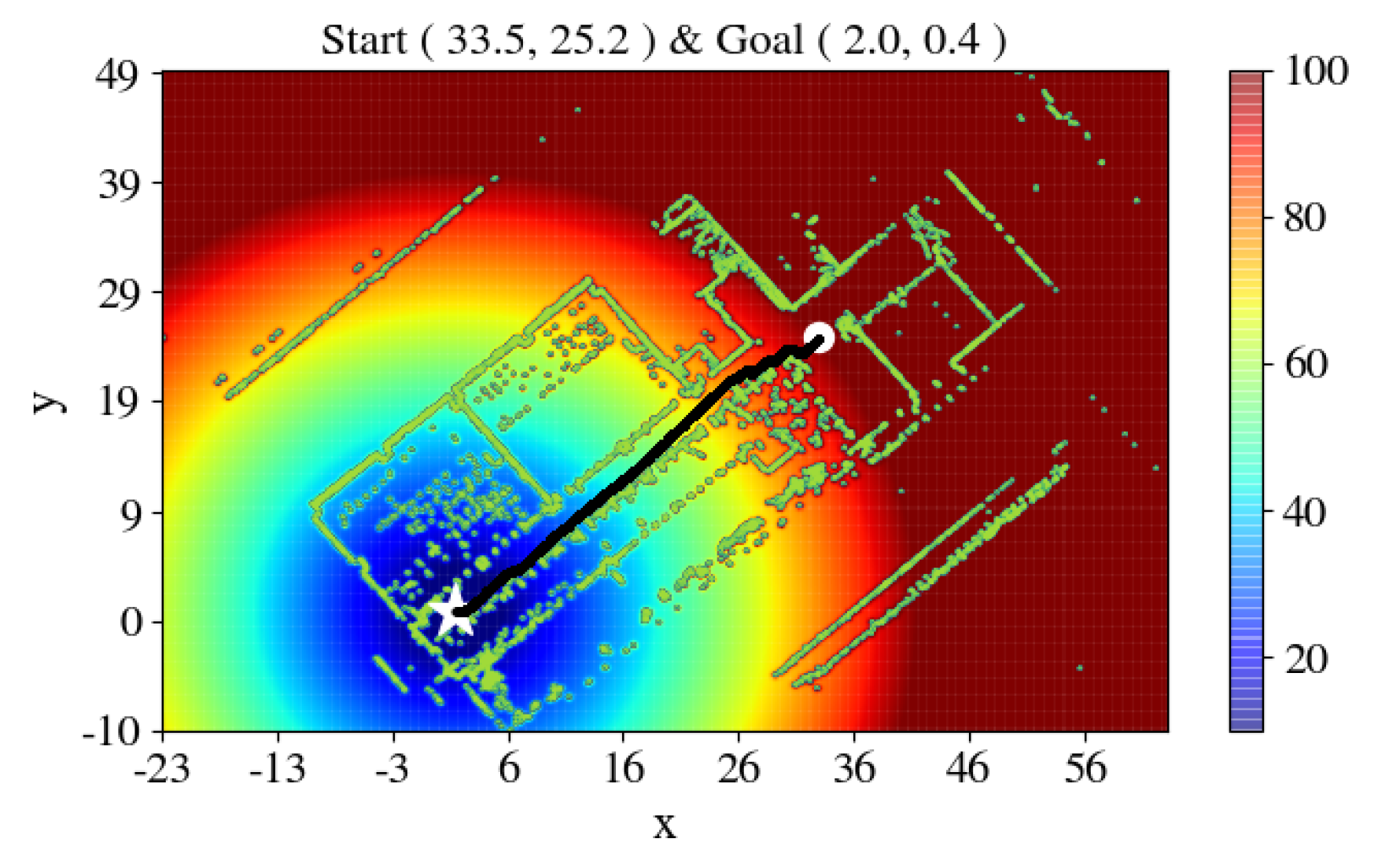
The next trial involves rounding up the transformed value. The
x-coordinate starting value is rounded up to 197. Thus, the next starting position is at (197, 133). The goal remains unchanged. The result is illustrated in
Figure 19.
It can be observed that a feasible path is found. The reason is that the 2D grid cell map is the scaled-down integer representation of the original 3D point cloud map. This also indicates that the size of the grid cell may affect the performance of the APF. Furthermore, as the consideration of the planner is based on the size of the discretized grid, the resulted path will ensure an added distance between the vehicle and any obstacle. The obtained path before and after smoothing is displayed in
Figure 20. Inverse transformation is applied to return the path to its original orientation.


