A Parametric Study of a Deep Reinforcement Learning Control System Applied to the Swing-Up Problem of the Cart-Pole

Abstract

In this investigation, the nonlinear swing-up problem associated with the cart-pole system modeled as a multibody dynamical system is solved by developing a deep Reinforcement Learning (RL) controller. Furthermore, the sensitivity analysis of the deep RL controller applied to the cart-pole swing-up problem is carried out. To this end, the influence of modifying the physical properties of the system and the presence of dry friction forces are analyzed employing the cumulative reward during the task. Extreme limits for the modifications of the parameters are determined to prove that the neural network architecture employed in this work features enough learning capability to handle the task under modifications as high as 90% on the pendulum mass, as well as a 100% increment on the cart mass. As expected, the presence of dry friction greatly affects the performance of the controller. However, a post-training of the agent in the modified environment takes only thirty-nine episodes to find the optimal control policy, resulting in a promising path for further developments of robust controllers.

1. Introduction

This section provides some necessary background material and emphasizes the significance of the present research. For this purpose, the formulation of the specific problem of interest for this investigation is set first. A concise literature review on the topics considered in this work is then reported for the benefit of the reader. More importantly, the scope and contributions of this paper are highlighted, whereas the structure of the manuscript is finally illustrated.

1.1. Background and Significance of the Research

The control of articulated mechanical systems relies on a high level of system understanding [1], expressed mainly through multibody dynamics models [2,3,4]. However, this approach is restrictive for systems with a high degree of complexity or uncertainty [5,6]. In particular, considering model-based control algorithms, such as the linear-quadratic regulator (LQR) and back-stepping (BS) techniques, the use of differential-algebraic equations of motion typical of the multibody approach is challenging. These heavily rely on model accuracy, which hinders their application to real platforms [7]. Therefore, the development of controllers for nonlinear systems is extremely challenging, time-consuming, and in many cases, an infeasible task. The traditional engineering approach consists of analytically deriving the system governing equations and manually adjusting the parameters of the control system to fit some measured physical parameters. Advanced expertise in applied mathematics, dynamical systems theory, computational methods, mathematical modeling, optimization frameworks, and operator-assisted algorithmic tuning of control parameters is then required.

1.2. Formulation of the Specific Problem of Interest for This Investigation

An alternative approach comes from the data-driven methods of Machine Learning (ML). Given the huge amount of data available, models for complex systems can be constructed by exploiting suitable ML techniques [8]. Besides, simulations and synthetic data for training allow employing neural networks in diverse applications with different degrees of complexity [8,9]. For instance, numerous authors have tried imitation learning to obtain motor skills from human demonstrations [10]. However, the resulting robotic skills are only near-optimal. One solution to this is the use of the Reinforcement Learning (RL) approach. This is an ML method that focuses on optimizing the Markov decision processes. The goal of RL is to learn how to control a system to maximize cumulative rewards. In contrast to supervised or unsupervised learning, this approach has samples generated dynamically with no clear labels, thereby considering only sparse reward signals [11]. In general, the optimization of an RL policy depends on the reward signal. It turns out to be effective when the reward can indicate which policy and single-action are better than others [12]. RL requires little prior knowledge to solve optimal control problems, with limited information about state dynamics and objective values [13,14,15]. In general, RL methods are computationally simple and represent an approach that is directly applicable to the control of nonlinear systems [16], combining the properties of optimal and adaptive controllers [17].

In the last decade, RL has had much success in the small discrete state-action space setting. Recently, through function approximation, it has been applied to problems with a large or continuous state space [18,19], in this way showing potential to be applied in disciplines as diverse as energy management [20,21], self-driving vehicles [22,23], and financial trend analysis [24,25]. Therefore, deep learning has become the mainstream way to obtain effective RL agent representations [26]. This is the so-called Deep RL (DRL), currently considered a promising approach for general artificial intelligence [11]. In recent times, DRL has also attracted much attention in robotics [27], where the agent becomes the robot controller, and the robot itself and its surroundings are the environment [28]. DRL in robotics is a control problem where a robot, the agent, acts in a stochastic environment by sequentially choosing actions over a sequence of time steps [29]. This framework allows a robotic agent to learn skills autonomously to solve tasks through trial and error [30]. However, robotic tasks are frequently high-dimensional in continuous state-action spaces [31], resulting in unfeasible amounts of interactions to obtain an optimized policy. For this reason, unfortunately, the workaround of discretizing the action space yields many limitations [29]. In general, the best outcomes for such environments are achieved considering value functions of the same nature [32]. However, the proof of convergence for these algorithms is just appearing in the literature [33,34].

Robustness against uncertainty in modeling has been one of the leading research subjects in control systems for the past twenty years [35]. This is mainly caused by the difficulties found when transferring a model to the real world. Usually, this is also due to the presence of oversimplified or non-modeled dynamic inaccuracies and the approximate numerical values of physical properties. From this perspective, the main advantage of RL is its ability to learn from interactions with the environment [36], finding an optimal control policy, rather than being programmed by a human designer [28]. However, the problem that arises in this domain is the poor convergence of RL based on neural networks, so far a great challenge for autonomous robots [37]. Besides, numerous physical interactions are usually unfeasible for these systems and lead to hardware wear and damage. Therefore, the more vulnerable the system, the more relevant is data-efficiency in learning. As discussed in this paper, a viable option is to train agents in simulated environments. However, accurate simulations come at the cost of high-dimensional observation and action spaces and complex intermittent contact interactions [27]. Regardless of the simulator accuracy, there is also a substantial difference between simulation and reality, the so-called reality-gap [38]. However, RL shows satisfactory results in simulated environments. Despite this fact, it has not been broadly applied in real physical systems like robots due to the fact that RL models trained in a simulation context normally come up short and need to be trained again in modified environments, which is hazardous and time-consuming [39].

1.3. Literature Review

The use of benchmark problems in the research and development of control systems is fundamental for analyzing a proposed system’s quality. Besides, this allows its comparison with other existing systems. Perhaps one of the most famous benchmarks in control development is the inverted pendulum system. Recently, a book on its use in control and robotics was published [40]. This is because, despite its structural simplicity, it is challenging to obtain a proper control law of the inverted pendulum system for many standard control techniques, in particular given its high nonlinearity, non-minimum phase, and underactuated nature. Research work on the inverted pendulum system focuses on developing controllers capable of swinging the pendulum while exhibiting robustness in the presence of external disturbances.

Multiple model-based control approaches are found in the literature considering the inverted pendulum benchmark. Nonlinear Model Predictive Control (NMPC) was employed in [41] for the swing-up of the parallel double inverted pendulum. The authors considered the Real-Time Iteration (RTI) scheme to allow the control to be implemented in hardware. In [42], the Integral Sliding Mode Control (ISMC) and the State-Dependent Riccati Equation (SDRE) were combined to perform the swing-up of the rotary inverted pendulum. The resulting robust continuous-time nonlinear optimal controller was experimentally tested. The work in [43] presented a Switched Robust Integral Sliding Mode (SRISM) control to address unmatched uncertainties. A Backstepping Sliding Mode Control (BSMC) scheme was proposed in [44] by transforming the dynamic system model into the so-called regular form. In this way, they took advantage of the convenient features that characterize the backstepping and sliding mode control schemes. A similar approach is that found in [45].

Many works have recently been reported in the literature for multiple types of nonlinear controllers featuring automatic tuning methodologies. In particular, metaheuristic algorithms to perform online tuning of the control parameters have been reported. For instance, Al-Araji presented a sliding mode control for the cart-pole system swing-up featuring the culture bees algorithm for online parameter tuning [46]. Su et al. complemented the hybrid sliding mode control by self-tuning the control parameters with the fireworks algorithm [47]. In addition, Mansoor and Bhutta considered the backstepping control scheme with the genetic algorithm for a similar scope [48]. Other authors considered the energy method to address the cart-pole swing-up control task. For instance, Singla and Singh considered this approach for the swing-up and switches to a Linear Quadratic Regulator Controller (LQRC) to stabilize in the vertical position [49].

In contrast to the mentioned model-based controllers, a model-free approach is that found in [50]. There, the energy method was employed in an online setup with no information of the system’s physical parameters. The algorithm self-learns a weight that is used in normalizing the energy injected to the pendulum. An approach considering neural networks to model the controller was presented in [51]. There, the swing-up problem of the double inverted pendulum was solved in a data-driven framework employing a neural network controller with parameters optimized via the hybrid uniform design multiobjective genetic algorithm. In [52], the Advantage Actor-Critic (A2C) was used to stabilize the cart-pole system [53]. This RL algorithm is considered in two different setups for the observations. One is with the state of the system, while the other employs a convolutional neural network to extract features from the animation produced by the simulation. Both cases consider a continuous observation space and a discrete control space. Recently, there has been interest in combining model-free and model-based approaches for controller development. Some works with this perspective are [54,55,56]. In these works, the RL was complemented with Proportional-Integral-Derivative (PID) controller, sliding mode control, and fuzzy logic, respectively.

The effect of the uncertainty in the friction coefficient on the controllers was analyzed in [57]. In this work, an NMPC and an RL based on temporal-difference (TD) were benchmarked under environments where the viscous friction, modeled as a damping force, was modified [58]. The effect of the uncertainty in the physical parameters of the cart-pole system was addressed briefly in [59]. There, the performance of an LQRC to balance the pole in the vertical position was evaluated when modifying the length of the pole.

1.4. Scope and Contributions of This Paper

The ML and deep RL techniques considered in this paper have great potential for mechanical engineering applications that are not well explored in the literature. Basically, there are two key points. First, RL methods allow for developing effective nonlinear controllers of mechanical systems that, to some extent, ignore the underlying physical behavior of the dynamical system to be controlled. In fact, the mechanical system to be controlled is treated as a black-box external environment from which input and output data are collected. This allows for using the same strategy for the control design in a large variety of state-space systems. As discussed in the paper, the control designer is called to develop an appropriate shape of the reward function that is more suitable for the engineering problem to be considered. Second, by using the post-training approach devised in this paper, one can design a robust control policy. Therefore, its performance is still satisfactory when some environment parameters are changed because of model uncertainty or due to other unpredictable phenomena. To investigate these two key points, a benchmark problem of nonlinear control is employed in the paper, namely the swing-up maneuver of the cart-pole system. The presence of dry friction is also considered to assess the robustness of the proposed approach. The difficulties related to traditional robust control systems with uncertainties in their physical parameters are often discussed in the literature. On the other hand, controllers based on reinforcement learning employ neural networks to represent the actuation policy. Thus, these present robust performance by virtue of the generalization capability of neural networks. Such robustness is exploited and improved in this work by employing a post-training of an optimal control policy in modified environments.

The study of the swing-up problem for the cart-pole system is one of the most common examples found in the literature as a benchmark problem to exemplify utilizing numerical experiments to test the effectiveness of a novel approach for designing a nonlinear controller. Thus, the scope and the contributions of this work are to study the robustness of an RL-based control system, specifically developed and applied to the swing-up task of the cart-pole system, and to address the issue of data efficiency in real-world implementations. This is performed through a parametric study of a trained policy represented by a multilayer perceptron. The main procedure consists of evaluating the behavior of the control system under modified environments that feature modifications of the cart-pole physical properties. This, to the best of the authors’ knowledge, was only briefly investigated in an RL controller with a simplified friction force approximated as damping in [57]. In contrast, the dry friction model employed in the present work is more accurate. Therefore, this paper is the first work in which the proposed control method based on deep reinforcement learning techniques is thoroughly developed and tested considering the dry friction phenomena. Additionally, modifications are considered for the mass of the cart, the mass and length of the pendulum, as well as the dry friction coefficient. These are varied in reasonable ranges to test the robustness of the control law devised in this paper. Besides, a method is proposed to further extend the agent capability in a data-efficient way by performing a subsequent training of the agent neural networks in a modified environment in the presence of dry friction. To this end, dry friction is modeled as a smoothed function of the instant normal force between the road and the environment. The findings of this work are based on extensive numerical experiments and result in a promising methodology for improvements in data efficiency and robustness for real systems’ implementation.

In this paper, a simplified, but realistic friction model is employed, namely viscous friction based on the hyperbolic tangent law, to perform the numerical experiments on the performance of the proposed controller. Consequently, some complex nonlinear features related to general friction phenomena, such as the stick-slip effect, the static friction, or, to some extent, the Stribeck curvature, are not captured by the present model. Although there is some loss of information by doing so, nonlinear viscous friction laws are widespread in engineering applications for implementing the analysis of articulated mechanical systems. In fact, in general, specific computational tools should be employed to consider the friction phenomena thoroughly. This mainly reflects using an appropriate numerical solution procedure for solving the equations of motion with discontinuous and fully nonlinear friction effects, at the expense of the computational time required to solve the set of ordinary differential equations. This is one of the main reasons why simplified versions of the friction model are preferred in engineering applications, such as linear and nonlinear friction laws. This is particularly true for the present work since, for each case considered in the paper, the differential equations of the cart-pole system must be solved a hundred times to run the deep reinforcement learning algorithms. Furthermore, in this paper, the effect of friction is mainly taken into account to demonstrate the effectiveness of a given controller designed in the absence of friction and subsequently post-trained to cope with its presence as an additional unmodeled disturbance phenomenon. Therefore, as mentioned before, in general, one should model friction forces considering more complete laws that better capture the phenomenon, but this is not functional or useful for the goals of the present investigation.

1.5. Organization of the Manuscript

The remainder of this paper is organized as follows. Section 2 elaborates on the theoretical framework of the RL algorithm employed and the experimental procedure proposed. Section 3 describes in detail the nonlinear model of the dynamical system under consideration and the setup of the numerical experiments. Section 4 reports the numerical results found for the environments considered, as well as some final remarks on the work done.

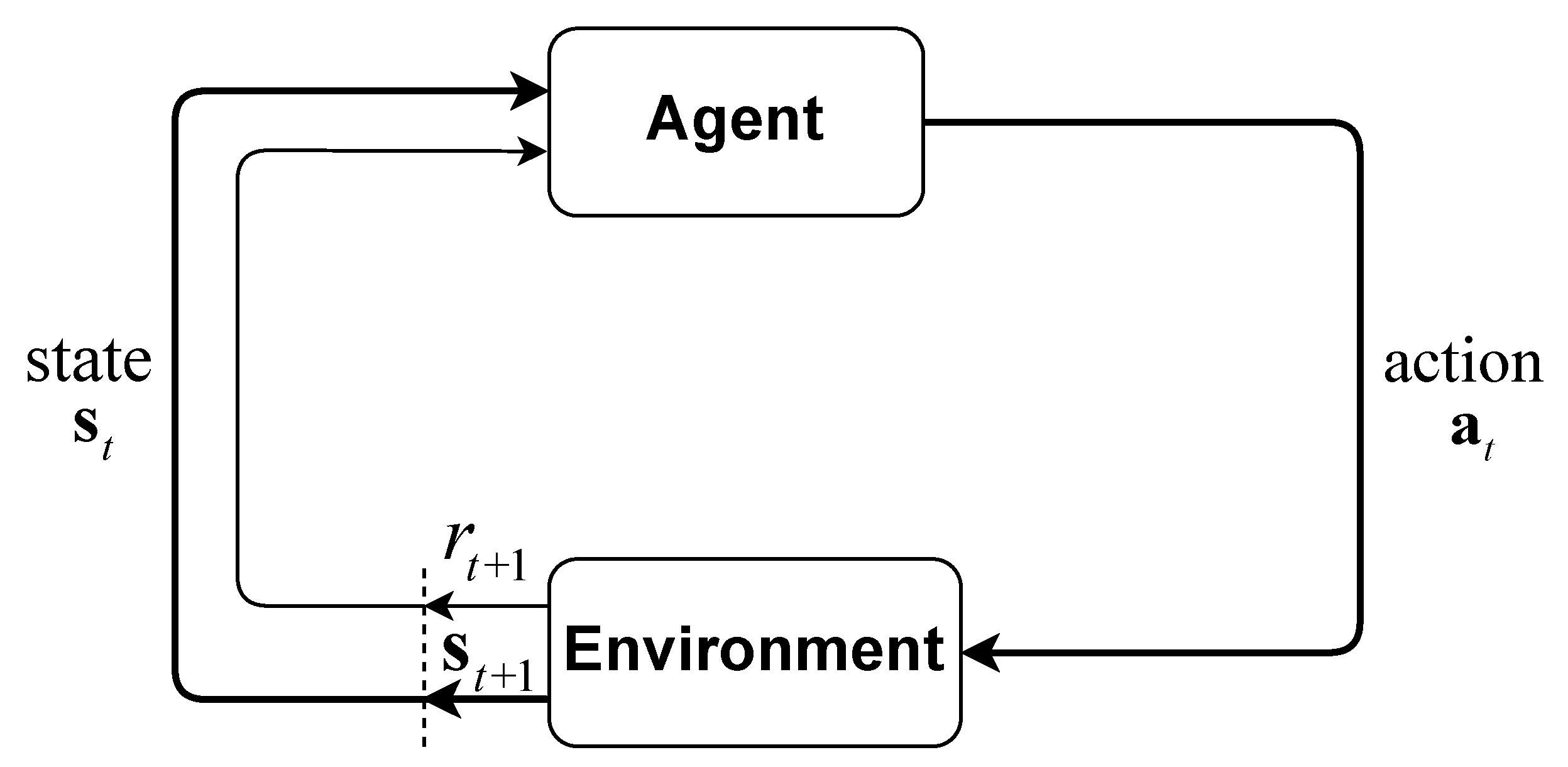
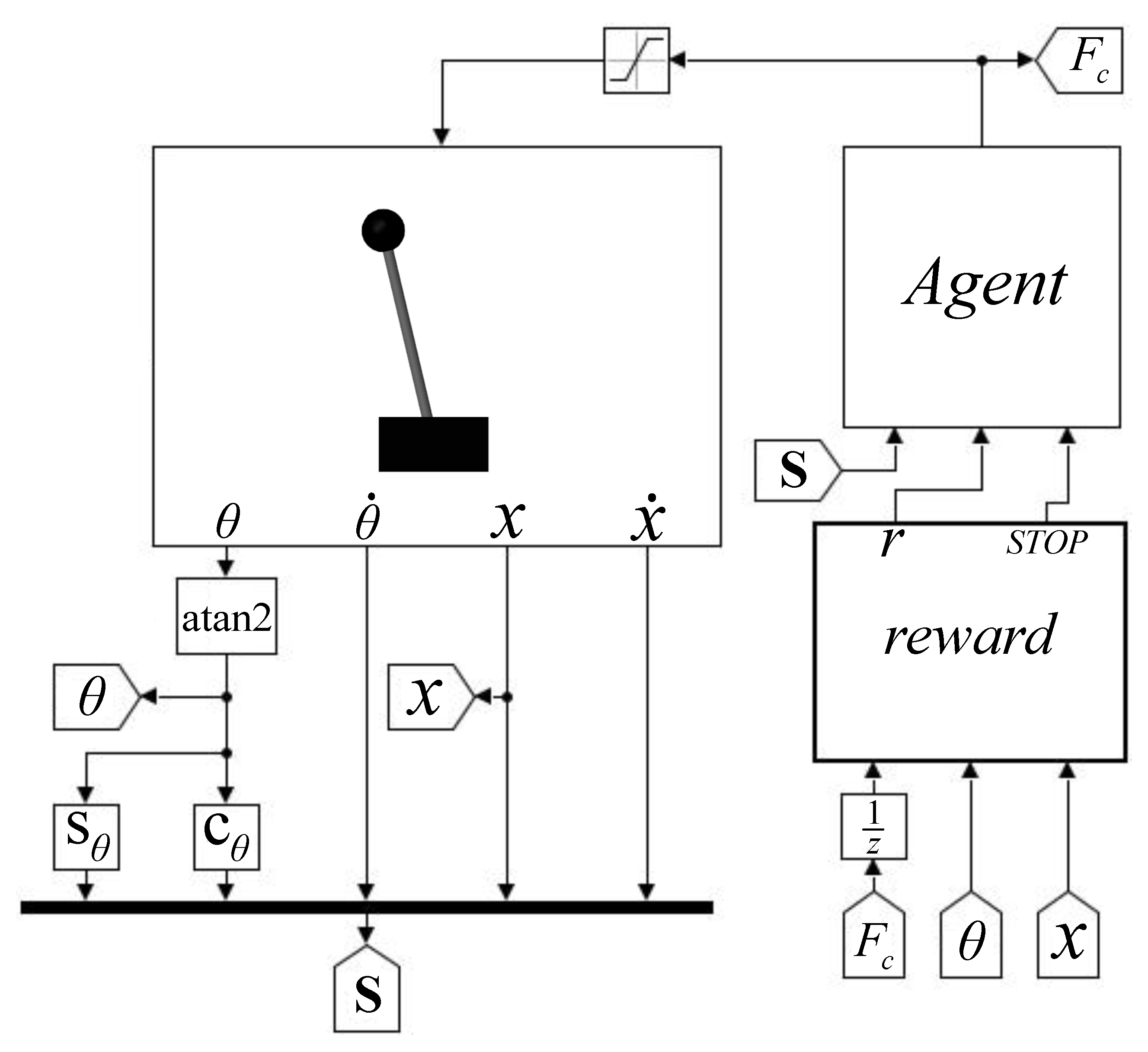
2. Research Methodology

RL is a data-driven approach to solve decision-making problems in the form of Markov Decision Processes (MDP). Figure 1 shows the workflow where an agent is fed with an observation $\mathbf{s}$ and a reward r so that it can decide an action $\mathbf{a}$ to take on an environment, with the scope of optimizing the cumulative reward $\sum r$ over time [60,61].

In this work, the algorithm used for training the agent is the Deep Deterministic Policy Gradient (DDPG) [62], an off-policy, model-free, actor-critic structured approach. The agent is composed of four neural networks, namely the Q-function ${\mathbf{Q}}_{\vartheta }$, the policy ${\mathit{\pi }}_{\phi }$, and their respective target lagged copies ${\mathbf{Q}}_{{\vartheta }^{\prime }}^{\prime }$ and ${\mathit{\pi }}_{{\phi }^{\prime }}^{\prime }$. The ${\mathbf{Q}}_{\vartheta }$ network is used to approximate the Q-function of the environment, that is the function predicting the cumulative reward for a given $\mathbf{s}$ and $\mathbf{a}$. The policy ${\mathit{\pi }}_{\phi }$ maps the state with an action. Each of the target copies contains lagged parameters of its corresponding neural network. The DDPG algorithm works through the joint learning of the optimal Q-function and the policy. The reinforcement learning loop begins with the random initialization of the four neural networks. Then, the agent begins to act in the environment to collect experiences in an experience buffer of dimension D. Each entry of the experience buffer is a tuple with the structure $\left(\mathbf{s},\mathbf{a},r,{\mathbf{s}}^{\prime }\right)$, where ${\mathbf{s}}^{\prime }$ represents the new state of the system after taking action $\mathbf{a}$. Then, in order to approximate the optimal Q-function, the Mean Squared Bellman Error (MSBE) is minimized by employing the loss function given by:

$$L_{MSBE}=\frac{1}{d}\sum _{i=1}^d{\left({\mathbf{Q}}_{\vartheta }({\mathbf{s}}_i,{\mathbf{a}}_i)-y_i({\mathbf{s}}_i,{\mathbf{a}}_i,r_i,{{\mathbf{s}}_i}^{\prime })\right)}^2$$

(1)

where ${\mathbf{Q}}_{\vartheta }(\mathbf{s},\mathbf{a})$ is the neural network with the current approximation of the optimal Q-function, d is the size of the replay buffer of previous experiences randomly sampled from the experience buffer of length D containing a subset of all the transitions in $\left(\mathbf{s},\mathbf{a},r,{\mathbf{s}}^{\prime }\right)$ tuples, ${\mathbf{s}}^{\prime }$ is the observation of the subsequent state, and $y_i$ is the target value function defined as:

$$y_i=\left\{\begin{array}{c}{r}_i+\gamma {\mathbf{Q}}_{{\vartheta }^{\prime }}^{\prime }\left({{\mathbf{s}}_i}^{\prime },{\mathit{\pi }}_{{\phi }^{\prime }}^{\prime }\left({{\mathbf{s}}_i}^{\prime }\right)\right),t<t_{end}\hfill \\ r_i,t=t_{end}\hfill \end{array}\right.$$

(2)

where t is the time of the observation ${\mathbf{s}}^{\prime }$, $t_{end}$ is the total duration of the episode of training, and $\gamma$ is the discount factor. In Equation (2), the target lagged copies ${\mathit{\pi }}_{{\phi }^{\prime }}^{\prime }\left({{\mathbf{s}}_i}^{\prime }\right)$ and $\mathbf{Q}{}_{{\vartheta }^{\prime }}^{\prime }\left({{\mathbf{s}}_i}^{\prime },{{\mathit{\pi }}^{\prime }}_{{\phi }^{\prime }}\left({{\mathbf{s}}_i}^{\prime }\right)\right)$ are used to avoid the instability in the training process derived from the recursive approach to approximate the Q-function. Then, the neural network ${\mathbf{Q}}_{\vartheta }$ is updated through the use of a one-step gradient by employing $L_{MSBE}$ defined in Equation (1). Subsequently, from the current ${\mathbf{Q}}_{\vartheta }$, the gradient ascent ∇ is computed to update the policy ${\mathit{\pi }}_{\phi }$. This is done by differentiating ${\mathbf{Q}}_{\vartheta }$ with respect to the parameters $\phi$ of ${\mathit{\pi }}_{\phi }$ while considering the parameters $\vartheta$ constants, leading to the following equation:

$$\nabla =\frac{1}{d}\sum _{i=1}^d{\nabla }_{{\mathit{\pi }}_{\phi }\left({\mathbf{s}}_i\right)}{\mathbf{Q}}_{\vartheta }\left({\mathbf{s}}_i,{\mathit{\pi }}_{\phi }\left({\mathbf{s}}_i\right)\right){\nabla }_{\phi }{\mathit{\pi }}_{\phi }\left({\mathbf{s}}_i\right)$$

(3)

Finally, the parameters ${\vartheta }^{\prime }$ and ${\phi }^{\prime }$ of the target neural networks ${\mathbf{Q}}_{{\vartheta }^{\prime }}^{\prime }$ and ${\mathit{\pi }}_{{\phi }^{\prime }}^{\prime }$ are updated by Polyak averaging with the parameter $\tau$ as:

$${\vartheta }^{\prime }=\tau \vartheta +(1-\vartheta ){\vartheta }^{\prime },{\phi }^{\prime }=\tau \phi +(1-\phi ){\phi }^{\prime }$$

(4)

This procedure is repeated until the optimal policy is found.

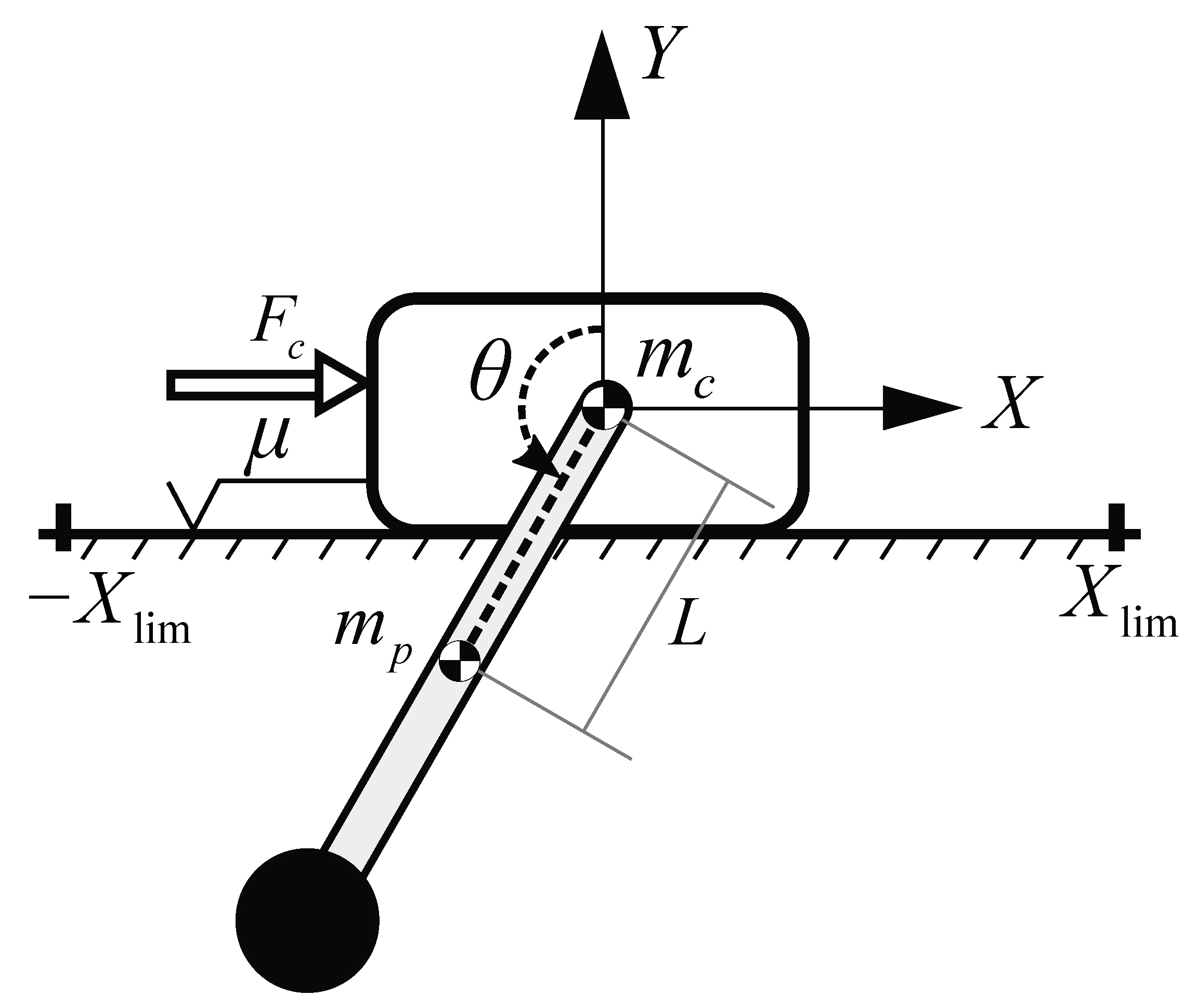
3. Dynamic Model Description and Numerical Experiments’ Setup

Recently, a plethora of benchmark problems has been used to evaluate the performance of RL algorithms. For instance, the Arcade Learning Environment [63,64] for discrete action space problems or OpenAI Gym [65], which considers benchmark control problems. Among the latter, there is the cart-pole swing-up [66], an underactuated, multivariable, inherently unstable, and strongly coupled nonlinear problem, which has been studied in the past by several authors [67]. When it comes to RL, the moderate level of complexity of the cart-pole system results in being advantageous due to its potential generalization to different domains, in contrast with other RL benchmarks such as the locomotion task [68,69], which requires highly specific algorithmic adaptations [70]. In this paper, the said system is chosen as a case study because its topological simplicity allows for performing a detailed study of the sensitivity of the developed controller in the presence of dry friction forces.

Figure 2 shows the scheme of the system, consisting of two rigid bodies, the cart with mass $m_c$, which moves along the X axis, and the pole with mass $m_p$, its centroidal moment of inertia $I_{zz,p}$ on the Z axis, and the center of mass positioned at a distance L from the revolute joint that allows the pendulum to rotate freely. The Lagrangian coordinates of the system are set as $\mathbf{q}={\left[\begin{array}{cc}x& \theta \end{array}\right]}^T$, and the corresponding equations of motion can be written as follows:

$$\mathbf{M}\ddot{\mathbf{q}}={\mathbf{Q}}_b$$

(5)

where $\ddot{\mathbf{q}}$ is the second time derivative of $\mathbf{q}$, whereas $\mathbf{M}$ and ${\mathbf{Q}}_b$ are respectively equal to:

$$\mathbf{M}=\left[\begin{array}{cc}{m}_c+m_p& -L{m}_{p}cos\left(\theta \right)\\ -L{m}_{p}cos\left(\theta \right)& m_p{L}^2+I_{zz,p}\end{array}\right]$$

(6)

$${\mathbf{Q}}_b=\left[\begin{array}{c}-{\dot{\theta }}^2{m}_{p}Lsin\left(\theta \right)+F_f+F_c\\ m_{p}gLsin\left(\theta \right)\end{array}\right]$$

(7)

where $F_c$ is the horizontal force the controller applies on the cart with the goal to swing-up the pole and $F_f$ is the friction force.

The modeling of dry friction in mechanical systems’ simulation plays a fundamental role. Considering this phenomenon in the early stages of engineering design is crucial to reduce the gap between numerical simulation and experimental results [71]. Multiple approaches to model dry friction exist in the literature, yet none of them has general validity [72]. The classical Coulomb dry friction model is widespread in engineering applications. The model considers that friction force opposes the motion and that its magnitude is independent of the contact area and velocity. Therefore, the dry friction force can be computed as:

$$F_{coul}=-\mu \left|F_N\right|sgn\left(\dot{x}\right)$$

(8)

where $\mu$ is the dry friction coefficient, $F_N$ is the instant normal force produced by the contact between the two surfaces interacting, and $\dot{x}$ is the relative velocity between them, whereas $sgn$ is the sign function defined as:

$$sgn\left(x\right)=\left\{\begin{array}{c}-1,x<0\hfill \\ 0,x=0\hfill \\ 1,x>0\hfill \end{array}\right.$$

(9)

Despite the apparent straightforwardness of the Coulomb friction model, for the implementation into dynamical systems simulation, it results in being challenging for numerical integration [71]. This is due to the friction force discontinuity at zero velocity, producing stiff equations of motion and the nonuniqueness and nonexistence of the solution for accelerations [72]. As a solution, the so-called smooth Coulomb friction model has been proposed [73]. It considers a smoothing function to remove the discontinuity. Multiple smoothing functions, such as linear, exponential, or trigonometric functions, have been employed in the literature. However, the smooth Coulomb friction model does not fully capture the physical phenomenon. This is because at zero velocity, the friction force is null. Therefore, it cannot reproduce stiction, the pre-sliding effect, or the Stribeck effect. Although there is a partial loss of information, nonlinear viscous friction laws such as the smooth Coulomb model are widespread in engineering applications devoted to implementing a quick but realistic analysis of articulated mechanical systems. More complex and accurate friction models can exhibit these effects, but require multiple additional physical parameters. In this work, given that the main interest is to perform a sensitivity analysis of the proposed control system, a smooth Coulomb friction model will be considered. Therefore, the dry friction force is given by:

$$F_f=-\mu \left|N\right|tanh\left(\dot{x}\right)$$

(10)

where $\mu$ is the dry friction coefficient, N is the instant normal force produced by the contact between the cart and the road, whereas the hyperbolic tangent is employed as an artificial function of the cart velocity necessary during the numerical simulations for smoothing the dry friction force described by the Coulomb law of friction. Figure 3 shows the Simulink implementation of the RL workflow, where the vector of observations $\mathbf{s}$ is defined as:

$$\mathbf{s}={\left[\begin{array}{ccccc}{\mathrm{s}}_{\theta }& {\mathrm{c}}_{\theta }& \dot{\theta }& x& \dot{x}\end{array}\right]}^T$$

(11)

where the abbreviations $sin\left(\theta \right)={\mathrm{s}}_{\theta }$ and $cos\left(\theta \right)={\mathrm{c}}_{\theta }$ are used.

The instant reward function for the environment is defined as follows:

$$r=\left\{\begin{array}{c}{r}_1,\left|x\right|\le x_{lim}\hfill \\ r_2,\left|x\right|>x_{lim}\hfill \end{array}\right.$$

(12)

where $x_{lim}$ is the maximum displacement allowed for the cart during the swing-up task, while $r_1$ and $r_2$ are defined as:

$$r_1=\left(A_r{\left|x\right|}^n+B_r{\left|\theta \right|}^n+C_r{\left|F_c\right|}^n\right)D_r$$

(13)

and:

$$r_2=r_1+E_r$$

(14)

where the constant parameters are respectively set as $A_r={10}^{-2}$, $B_r={10}^{-1}$, $C_r=5$, $D_r=-{10}^{-2}$, $E_r=-{10}^2$, and $n=2$. The shape of the reward function allows for penalizing the magnitude of x, $\theta$, and $F_c$. Therefore, the optimal policy will be that in which the system manages to perform the swing-up with the lowest force possible, and the cart is in the initial position at the end of the task. On the other hand, the actor ${\mathit{\pi }}_{\phi }$ and critic ${\mathbf{Q}}_{\vartheta }$ neural networks are multilayer perceptrons with architectures as respectively shown in (a) and (b) of Figure 4.

The training process of the agent is done employing the DDPG algorithm under the following restrictions:

$$\begin{array}{cc}{F}_c\le F_{max},& \left|x\right|\end{array}\le x{}_{lim},t\le t_f$$

(15)

where $F_{max}$ is the maximum force allowed to the controller, set to 20 (N), $x_{lim}$ is the maximum lateral displacement of the cart, equal to 1 (m), and $t_f$ is the maximum duration of the task, set to 25 (s). Then, the sensitivity analysis of the controller consists of evaluating its performance under modified environments featuring variations of the physical properties of the system. Finally, to expand the optimal behavior space for the agent, a post-training of its structural parameters is performed in a modified environment.

4. Numerical Results and Discussion

In this section, the results obtained from the parametric analysis are reported. In total, thirteen different cases of modified environments are considered. The remainder of the section is organized as follows. Section 4.1 shows the results obtained for the parametric study where the physical properties of the system, namely the masses and geometry, are modified, and no presence of dry friction is considered. Section 4.2 reports the results regarding the effect of the dry friction presence and its corresponding variation on the agent, as well as the results arising from the post-training method. Section 4.3 provides some general final remarks and a concise discussion of the numerical results found.

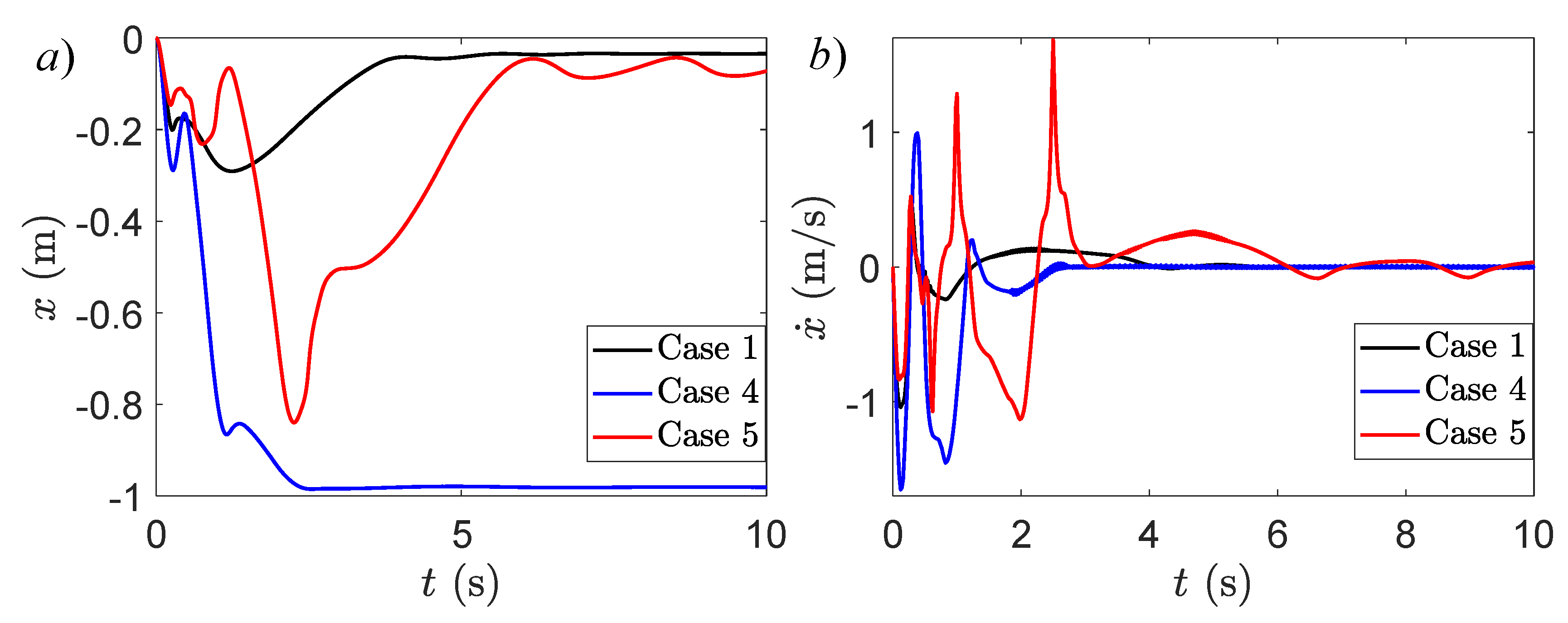
4.1. Physical Properties’ Parameter Study

The hyperparameters for the neural networks learning and DDPG algorithm employed for the training of the agent are mentioned in

Table 1. Neural networks and Deep Deterministic Policy Gradient (DDPG) hyperparameters for the training.

Symbol	Meaning	Value
	Actor learning rate	$5\times {10}^{-4}$
	Critic learning rate	${10}^{-3}$
	Gradient threshold	$1.00$
D	Experience buffer length	${10}^6$
d	Replay buffer size	$128.00$
$\tau$	Polyak averaging factor	${10}^{-3}$
$\gamma$	Value function discount factor	$0.99$
$t_s$	Sampling time	$0.02$ s

, and the corresponding learning curves are shown in (a) and (b) of Figure 5.

The optimal policy is found at Episode 435 considering the criteria $r_{avg}>-80$, and $r_{avg}$ is the average cumulative reward in a window of five episodes.

Table 2. Cases of the sensitivity analysis of agent A without the presence of dry friction $(\mu =0)$.

Case	${\mathit{m}}_{\mathit{c}}$ (kg)	${\mathit{m}}_{\mathit{p}}$ (kg)	L (m)	${\mathit{T}}_{\mathit{su}}$ (s)	$\sum \mathit{r}$
1	1.00	1.00	0.10	0.98	−71.55
2	0.06	1.00	0.10	1.54	−233.93
3	2.00	1.00	0.10	5.1	−269.89
4	1.00	0.10	0.10	1.70	−204.93
5	1.00	1.90	0.1	3.30	−205.93
6	1.00	1.00	0.07	1.70	−262.46
7	1.00	1.00	0.19	3.42	−197.49
8	0.65	0.65	0.06	1.44	−226.57
9	1.25	1.25	0.12	1.28	−201.23

reports the properties of the environments considered, where no dry friction is present.

For the purposes of the present work, the swing-up time is defined according to the following formula:

$$\begin{array}{c}\mathrm{if}\left|\theta \right|<A_l\mathrm{and}\left|\theta \right|\ge B_l\mathrm{and}\left|\dot{\theta }\right|\le C_l\mathrm{and}\left|\dot{x}\right|\le D_l\hfill \\ T_{su}=t\hfill \\ \mathrm{else}\hfill \\ T_{su}=0\hfill \\ \mathrm{end}\hfill \end{array}$$

(16)

where t is the time variable, $T_{su}$ is the swing-up time, x is the cart linear displacement, $\theta$ is the pendulum angular displacement, $\dot{x}$ is the cart linear velocity, $\dot{\theta }$ is the pendulum angular velocity, while $A_l=5(deg)$, $B_l=0(deg)$, $C_l=0.1\left(\mathrm{rad}/\phantom{\mathrm{rad}\mathrm{s}}\mathrm{s}\right)$, and $D_l=0.5\left(\mathrm{m}/\phantom{\mathrm{m}\mathrm{s}}\mathrm{s}\right)$ are limit constants.

The training is carried out in the environment of Case 1, producing the agent A. The remaining cases report the performance of agent A in each defined environment. The magnitudes for the physical properties are the extreme values for which agent A manages to perform the swing-up under the conditions mentioned in Equation (15). In particular, Cases 2 to 7 report individual variations of the three physical parameters $m_c$, $m_p$, and L where, based on the cumulative reward obtained during the task, it is found that the increase in $m_c$ has the greatest impact on the agent performance. An interesting effect is observed in Cases 4 and 5, where the respective 90% increase and decrease in $m_p$ yield close cumulative rewards. Figure 6 and Figure 7 show the state response of agent A in Cases 1, 4, and 5.

It can be seen that, even though the cumulative rewards reported in Table 2 for Cases 4 and 5 are close, in general, the best output takes place in Case 4, which performs a swing-up in a shorter time without the presence of full rotations of the pole, in contrast with Case 5. Therefore, the pendulum mass $m_p$ is the parameter with the least impact on the agent performance. Cases 8 and 9 consider joint equal changes of the three physical properties, a decrease of 35% and an increase of 25%, respectively. Figure 8 and Figure 9 show the response of agent A in Cases 1, 8, and 9, where even though the latter is the more inertial one, its response yields a better reward than Case 8, as shown in Figure 10.

This is due to the oscillating pattern of $F_c$ in Case 8 shown in (a) of Figure 10. Therefore, the agent performance is more susceptible to joint equal inertial decreases.

4.2. Dry Friction Parameter Study

A subsequent analysis considers the effect of the presence of dry friction on the performance of agent A. Case 10 of

Table 3. Cases of the sensitivity analysis of the dry friction influence on the agent performance.

Case	Agent	$\mathit{\mu }$	${\mathit{m}}_{\mathit{c}}$ (kg)	${\mathit{m}}_{\mathit{p}}$ (kg)	L (kg)	${\mathit{T}}_{\mathit{su}}$ (s)	$\sum \mathit{r}$
10	A	0.30	1.00	1.00	0.10	-	−341.48
11	B	0.30	1.00	1.00	0.10	2.00	−74.71
12	B	0	1.00	1.00	0.10	2.74	−81.51
13	B	0.80	1.00	1.00	0.10	0.80	−78.55

proves the impact of this phenomenon to be high since the cumulative reward drops sharply, and the system has an unstable response.

In Case 10 of Table 3, the swing-up has not been achieved; therefore, no swing-up time is reported. Apart from Figure 11, this is also shown in Figure 12 and Figure 13, where the swing-up is performed only for short periods.

Additional training is performed on agent A in an environment with the properties of Case 11 in Table 3, and the corresponding learning curves are shown in (a) and (b) of Figure 11. The optimal policy is found after 39 training episodes, and the resulting agent is called agent B, featuring optimal performance with or without the presence of dry friction, as well as with high increments of the dry friction coefficient, as shown in Cases 12 and 13 of Table 3.

4.3. Discussion and Final Remarks

The starting point of this work is the formulation of a multibody model of the cart-pole system that can be easily manipulated by controlling an external force applied to the cart. This dynamic model is sufficiently complex to exhibit an interesting nonlinear behavior during the swing-up task and, at the same time, sufficiently simple to be used for a parametric study of the robustness and/or sensitivity of a nonlinear control law devised by using a deep RL method. Furthermore, the presence of dry friction, often erroneously neglected in robotic applications leading to the origination of unwanted dynamic phenomena, is taken into account in this investigation. As expected, the presence of dry friction has a great impact on the performance of the controller devised by employing the deep RL approach. Implementing the modified environment and performing a post-training procedure for the agent resulting from the original design require only a small set of thirty-nine additional episodes to generate the optimal control policy for environments with or without the dry friction presence. For instance, agent B can indeed do the swing-up in an environment with and without dry friction, as shown in Case 12 of Table 3. Thereby, this approach provides a promising path for further developments.

Based on the impact of the modified environments on the performance of the agents A and B devised in this work, it is concluded that the RL-based control system is robust. In particular, the maximum percentage of change achieved by performing the task correctly is up to 90% in the pendulum mass $m_p$ alone, 94% in the cart mass $m_c$ alone, and up to 25% for the two parameters together. Additionally, as shown in the manuscript, the proposed post-training of the agent carried out in an environment with dry friction required only thirty-nine episodes to find the optimal policy, thereby being robust enough to work optimally in the presence of dry friction with its coefficient increased up to 50% or equal to zero. Therefore, the numerical experiments performed in this investigation prove the transfer learning approach to be promising for the reality-gap problem found in robotics.

Nonlinear model-based control systems, such as [41,42,43,44], to name a few, do not consider dry friction since the complexity of the resulting model is restrictive. In contrast, a model-free approach like the one in this work, based on deep RL, allows us to consider such a phenomenon. Additionally, given the generalization capability of neural networks, the robustness of the system to the uncertainty in the physical parameters is high, as shown by the numerical results of the sensitivity analysis carried out. This, to the best of the authors’ knowledge, has not been previously done in the literature. Furthermore, said robustness can be increased with the post-training proposed and numerically tested in the present work.

The developed control system has limitations related to the simplifications used in the dry friction model present in the environment during training. This is because physical effects, such as stiction, the pre-sliding, and the Stribeck effect, cannot be reproduced using the smooth Coulomb friction model. Additionally, the agent capacity can be extended by running training episodes in a subsequent session in an experimental setting. Said implementation is feasible given the sampling time used during training and the performance required by an actuator, both within commercial hardware margins. This is also demonstrated by the presence in the literature of several alternative investigations on the practical methods for controlling the cart-pole system that were also tested experimentally using a dedicated test rig.

The friction model considered was used to exemplify the effect of a modified environment. Furthermore, the dry friction model employed was chosen for the sake of simplicity and clarity, to avoid the ambiguity in the non-uniqueness of the resulting acceleration arising from the discontinuity of the friction force at zero velocity that is typical of the Coulomb model and also because other more advanced friction models require multiple parameters for their correct definition and functioning [71]. The sensitivity analysis performed showed a high parameters space where the controller could perform the task required. For a physical system with higher complexity compared to the model considered in the paper, which features multiple physical parameters and phenomena involved, it would be required to consider an in-detail statistical approach, such as the two-level factorial analysis, which is clearly outside of the scope of the present work.

5. Summary and Conclusions

The authors’ research focuses on designing, modeling, and controlling mechanical systems subjected to complex force fields [74,75]. Therefore, the mutual interactions between multibody system dynamics, applied system identification, and nonlinear control fall within the scope of the authors’ research domain. In this work, on the other hand, the sensitivity analysis of a deep Reinforcement Learning (RL) controller applied to the cart-pole swing-up problem is performed. Through extensive numerical experiments, the effectiveness of the proposed controller is analyzed in the case of the presence of friction forces. Subsequent works will focus on studying environments characterized by randomized parameters during the training procedure to further improve the robustness of the resulting control system.

Future research works will be devoted to further refining the numerical procedure for developing the control algorithm proposed in this paper, so that it can be readily applied to more complex dynamical systems, such as articulated mechanical systems modeled within the multibody framework that have an underactuated structure. For instance, an immediate extension of this work, which is focused on the swing-up problem of a cart-pole system, is the development of a robust controller similarly based on the use of the deep RL approach for the Furuta pendulum, as well as for an inverted pendulum controlled through a gyroscope mounted on a gimbal. In fact, the benchmark problems mentioned before are closer to practical systems employed in engineering applications, and the development of a robust controller for such systems seems quite promising.

In summary, the current research work focuses on the computational aspects of the swing-up problem of the cart-pole system. The paper aims to develop a nonlinear controller based on reinforcement learning techniques simulated in a virtual environment. Therefore, the experimental verification using a test-rig of the proposed controller is outside the scope of the present work. However, this issue will be addressed in future investigations specifically dedicated to developing experimental results for supporting the theoretical controller obtained using the proposed approach. Additionally, the development of an in-depth analysis of the DRL-based the sensitivity and robustness of the control system and its experimental implementation, using advanced dry friction models capable of exhibiting stiction, the pre-sliding, and the Stribeck effect, are topics that will be considered as future extensions of the present work.

References

1. Hesse, M.; Timmermann, J.; Hüllermeier, E.; Trächtler, A. A Reinforcement Learning Strategy for the Swing-Up of the Double Pendulum on a Cart. Procedia Manuf. 2018, 24, 15. [Google Scholar] [CrossRef]
2. Manrique, C.; Pappalardo, C.M.; Guida, D. A Model Validating Technique for the Kinematic Study of Two-Wheeled Vehicles. Lect. Notes Mech. Eng. 2019, 549–558. [Google Scholar] [CrossRef]
3. Pappalardo, C.M.; De Simone, M.C.; Guida, D. Multibody modeling and nonlinear control of the pantograph/catenary system. Arch. Appl. Mech. 2019, 89, 1589–1626. [Google Scholar] [CrossRef]
4. Pappalardo, C.; Guida, D. Forward and Inverse Dynamics of a Unicycle-Like Mobile Robot. Machines 2019, 7, 5. [Google Scholar] [CrossRef] [Green Version]
5. Villecco, F.; Pellegrino, A. Evaluation of Uncertainties in the Design Process of Complex Mechanical Systems. Entropy 2017, 19, 475. [Google Scholar] [CrossRef] [Green Version]
6. Villecco, F.; Pellegrino, A. Entropic Measure of Epistemic Uncertainties in Multibody System Models by Axiomatic Design. Entropy 2017, 19, 291. [Google Scholar] [CrossRef] [Green Version]
7. Hu, D.; Pei, Z.; Tang, Z. Single-Parameter-Tuned Attitude Control for Quadrotor with Unknown Disturbance. Appl. Sci. 2020, 10, 5564. [Google Scholar] [CrossRef]
8. Talamini, J.; Bartoli, A.; De Lorenzo, A.D.; Medvet, E. On the Impact of the Rules on Autonomous Drive Learning. Appl. Sci. 2020, 10, 2394. [Google Scholar] [CrossRef] [Green Version]
9. Sharifzadeh, S.; Chiotellis, I.; Triebel, R.; Cremers, D. Learning to drive using inverse reinforcement learning and deep q-networks. arXiv 2016, arXiv:1612.03653. [Google Scholar]
10. Cho, N.J.; Lee, S.H.; Kim, J.B.; Suh, I.H. Learning, Improving, and Generalizing Motor Skills for the Peg-in-Hole Tasks Based on Imitation Learning and Self-Learning. Appl. Sci. 2020, 10, 2719. [Google Scholar] [CrossRef] [Green Version]
11. Zhang, H.; Qu, C.; Zhang, J.; Li, J. Self-Adaptive Priority Correction for Prioritized Experience Replay. Appl. Sci. 2020, 10, 6925. [Google Scholar] [CrossRef]
12. Hong, D.; Kim, M.; Park, S. Study on Reinforcement Learning-Based Missile Guidance Law. Appl. Sci. 2020, 10, 6567. [Google Scholar] [CrossRef]
13. Rivera, Z.B.; De Simone, M.C.; Guida, D. Unmanned Ground Vehicle Modelling in Gazebo/ROS-Based Environments. Machines 2019, 7, 42. [Google Scholar] [CrossRef] [Green Version]
14. De Simone, M.C.; Guida, D. Control design for an under-actuated UAV model. FME Trans. 2018, 46, 443–452. [Google Scholar] [CrossRef]
15. Murray, R.; Palladino, M. A model for system uncertainty in reinforcement learning. Syst. Control Lett. 2018, 122, 24–31. [Google Scholar] [CrossRef] [Green Version]
16. Sutton, R.S.; Barto, A.G.; Williams, R.J. Reinforcement learning is direct adaptive optimal control. IEEE Control Syst. 1992, 12, 19–22. [Google Scholar] [CrossRef]
17. Cheng, Q.; Wang, X.; Niu, Y.; Shen, L. Reusing Source Task Knowledge via Transfer Approximator in Reinforcement Transfer Learning. Symmetry 2018, 11, 25. [Google Scholar] [CrossRef] [Green Version]
18. Nichols, B.D. Continuous Action-Space Reinforcement Learning Methods Applied to the Minimum-Time Swing-Up of the Acrobot. In Proceedings of the 2015 IEEE International Conference on Systems, Man, and Cybernetics, Hong Kong, China, 9–12 October 2015; pp. 2084–2089. [Google Scholar]
19. Lesort, T.; Díaz-Rodríguez, N.; Goudou, J.-F.; Filliat, D. State representation learning for control: An overview. Neural Netw. 2018, 108, 379–392. [Google Scholar] [CrossRef] [Green Version]
20. Oh, E. Reinforcement-Learning-Based Virtual Energy Storage System Operation Strategy for Wind Power Forecast Uncertainty Management. Appl. Sci. 2020, 10, 6420. [Google Scholar] [CrossRef]
21. Phan, B.C.; Lai, Y.-C. Control Strategy of a Hybrid Renewable Energy System Based on Reinforcement Learning Approach for an Isolated Microgrid. Appl. Sci. 2019, 9, 4001. [Google Scholar] [CrossRef] [Green Version]
22. Kővári, B.; Hegedüs, F.; Bécsi, T. Design of a Reinforcement Learning-Based Lane Keeping Planning Agent for Automated Vehicles. Appl. Sci. 2020, 10, 7171. [Google Scholar] [CrossRef]
23. Tran, D.Q.; Bae, S.-H. Proximal Policy Optimization Through a Deep Reinforcement Learning Framework for Multiple Autonomous Vehicles at a Non-Signalized Intersection. Appl. Sci. 2020, 10, 5722. [Google Scholar] [CrossRef]
24. Sattarov, O.; Muminov, A.; Lee, C.W.; Kang, H.K.; Oh, R.; Ahn, J.; Oh, H.J.; Jeon, H.S. Recommending Cryptocurrency Trading Points with Deep Reinforcement Learning Approach. Appl. Sci. 2020, 10, 1506. [Google Scholar] [CrossRef] [Green Version]
25. Rundo, F. Deep LSTM with Reinforcement Learning Layer for Financial Trend Prediction in FX High Frequency Trading Systems. Appl. Sci. 2019, 9, 4460. [Google Scholar] [CrossRef] [Green Version]
26. Chen, H.; Liu, Y.; Zhou, Z.; Zhang, M. A2C: Attention-Augmented Contrastive Learning for State Representation Extraction. Appl. Sci. 2020, 10, 5902. [Google Scholar] [CrossRef]
27. Xiang, G.; Su, J. Task-Oriented Deep Reinforcement Learning for Robotic Skill Acquisition and Control. IEEE Trans. Cybern. 2019, 1–14. [Google Scholar] [CrossRef] [PubMed]
28. Wawrzyński, P. Control Policy with Autocorrelated Noise in Reinforcement Learning for Robotics. Int. J. Mach. Learn. Comput. 2015, 5, 91–95. [Google Scholar] [CrossRef] [Green Version]
29. Beltran-Hernandez, C.C.; Petit, D.; Ramirez-Alpizar, I.G.; Harada, K. Variable Compliance Control for Robotic Peg-in-Hole Assembly: A Deep-Reinforcement-Learning Approach. Appl. Sci. 2020, 10, 6923. [Google Scholar] [CrossRef]
30. Moreira, I.; Rivas, J.; Cruz, F.; Dazeley, R.; Ayala, A.; Fernandes, B. Deep Reinforcement Learning with Interactive Feedback in a Human–Robot Environment. Appl. Sci. 2020, 10, 5574. [Google Scholar] [CrossRef]
31. Williams, G.; Wagener, N.; Goldfain, B.; Drews, P.; Rehg, J.M.; Boots, B.; Theodorou, E.A. Information theoretic MPC for model-based reinforcement learning. In Proceedings of the 2017 IEEE International Conference on Robotics and Automation (ICRA), Singapore, 29 May–3 June 2017; pp. 1714–1721. [Google Scholar]
32. Anderson, C.W.; Lee, M.; Elliott, D.L. Faster reinforcement learning after pretraining deep networks to predict state dynamics. In Proceedings of the 2015 International Joint Conference on Neural Networks (IJCNN), Killarney, Ireland, 12–16 July 2015; Volume 2015, pp. 1–7. [Google Scholar]
33. Lee, M.; Anderson, C.W. Convergent reinforcement learning control with neural networks and continuous action search. In Proceedings of the 2014 IEEE Symposium on Adaptive Dynamic Programming and Reinforcement Learning (ADPRL), Orlando, FL, USA, 9–12 December 2014; pp. 1–8. [Google Scholar]
34. Maei, H.R.; Szepesvari, C.; Bhatnagar, S.; Precup, D.; Silver, D.; Sutton, R.S. Convergent temporal-difference learning with arbitrary smooth function approximation. In Proceedings of the 22nd International Conference on Neural Information Processing Systems, Vancouver, BC, Canada, 7–10 December 2009; pp. 1204–1212. [Google Scholar]
35. Morimoto, J.; Doya, K. Robust Reinforcement Learning. Neural Comput. 2005, 17, 335–359. [Google Scholar] [CrossRef] [PubMed]
36. François-Lavet, V.; Henderson, P.; Islam, R.; Bellemare, M.G.; Pineau, J. An Introduction to Deep Reinforcement Learning. Found. Trends Mach. Learn. 2018, 11, 219–354. [Google Scholar] [CrossRef] [Green Version]
37. Yang, Y.; Li, X.; Zhang, L. Task-specific pre-learning to improve the convergence of reinforcement learning based on a deep neural network. In Proceedings of the 2016 12th World Congress on Intelligent Control and Automation (WCICA), Guilin, China, 12–15 June 2016; Volume 2016, pp. 2209–2214. [Google Scholar]
38. Zagal, J.C.; Ruiz-del-Solar, J.; Vallejos, P. Back to reality: Crossing the reality gap in evolutionary robotics. IFAC Proc. Vol. 2004, 37, 834–839. [Google Scholar] [CrossRef]
39. Bekar, C.; Yuksek, B.; Inalhan, G. High Fidelity Progressive Reinforcement Learning for Agile Maneuvering UAVs. In Proceedings of the AIAA Scitech 2020 Forum; American Institute of Aeronautics and Astronautics, Orlando, FL, USA, 6–10 January 2020; pp. 1–12. [Google Scholar]
40. Boubaker, O.; Iriarte, R. (Eds.) The Inverted Pendulum in Control Theory and Robotics: From Theory to New Innovations; IET: London, UK, 2017; Volume 111, ISBN 978-1-78561-321-0. [Google Scholar]
41. Gonzalez, O.; Rossiter, A. Fast hybrid dual mode NMPC for a parallel double inverted pendulum with experimental validation. IET Control Theory Appl. 2020, 14, 2329–2338. [Google Scholar] [CrossRef]
42. Nekoo, S.R. Digital implementation of a continuous-time nonlinear optimal controller: An experimental study with real-time computations. ISA Trans. 2020, 101, 346–357. [Google Scholar] [CrossRef]
43. Zhang, X.; Xiao, L.; Li, H. Robust Control for Switched Systems with Unmatched Uncertainties Based on Switched Robust Integral Sliding Mode. IEEE Access 2020, 8, 138396–138405. [Google Scholar] [CrossRef]
44. Ullah, S.; Khan, Q.; Mehmood, A.; Bhatti, A.I. Robust Backstepping Sliding Mode Control Design for a Class of Underactuated Electro–Mechanical Nonlinear Systems. J. Electr. Eng. Technol. 2020, 15, 1821–1828. [Google Scholar] [CrossRef]
45. Khan, Q.; Akmeliawati, R.; Bhatti, A.I.; Khan, M.A. Robust stabilization of underactuated nonlinear systems: A fast terminal sliding mode approach. ISA Trans. 2017, 66, 241–248. [Google Scholar] [CrossRef]
46. Al-Araji, A.S. An adaptive swing-up sliding mode controller design for a real inverted pendulum system based on Culture-Bees algorithm. Eur. J. Control 2019, 45, 45–56. [Google Scholar] [CrossRef]
47. Su, T.-J.; Wang, S.-M.; Li, T.-Y.; Shih, S.-T.; Hoang, V.-M. Design of hybrid sliding mode controller based on fireworks algorithm for nonlinear inverted pendulum systems. Adv. Mech. Eng. 2017, 9, 1–13. [Google Scholar] [CrossRef] [Green Version]
48. Mansoor, H.; Bhutta, H.A. Genetic algorithm based optimal back stepping controller design for stabilizing inverted pendulum. In Proceedings of the 2016 International Conference on Computing, Electronic and Electrical Engineering (ICE Cube), Quetta, Pakistan, 11–12 April 2016; pp. 6–9. [Google Scholar]
49. Singla, A.; Singh, G. Real-Time Swing-up and Stabilization Control of a Cart-Pendulum System with Constrained Cart Movement. Int. J. Nonlinear Sci. Numer. Simul. 2017, 18, 525–539. [Google Scholar] [CrossRef]
50. Dındış, G.; Karamancıoğlu, A. A Self-learning Robust Swing-up algorithm. Trans. Inst. Meas. Control 2016, 38, 395–401. [Google Scholar] [CrossRef]
51. Al-Janan, D.H.; Chang, H.-C.; Chen, Y.-P.; Liu, T.-K. Optimizing the double inverted pendulum’s performance via the uniform neuro multiobjective genetic algorithm. Int. J. Autom. Comput. 2017, 14, 686–695. [Google Scholar] [CrossRef]
52. Zheng, Y.; Li, X.; Xu, L. Balance Control for the First-order Inverted Pendulum Based on the Advantage Actor-critic Algorithm. Int. J. Control. Autom. Syst. 2020. [Google Scholar] [CrossRef]
53. Mnih, V.; Badia, A.P.; Mirza, M.; Graves, A.; Lillicrap, T.P.; Harley, T.; Silver, D.; Kavukcuoglu, K. Asynchronous Methods for Deep Reinforcement Learning. arXiv 2016, arXiv:1602.01783. [Google Scholar]
54. Kim, J.-B.; Lim, H.-K.; Kim, C.-M.; Kim, M.-S.; Hong, Y.-G.; Han, Y.-H. Imitation Reinforcement Learning-Based Remote Rotary Inverted Pendulum Control in OpenFlow Network. IEEE Access 2019, 7, 36682–36690. [Google Scholar] [CrossRef]
55. Dao, P.N.; Liu, Y.-C. Adaptive Reinforcement Learning Strategy with Sliding Mode Control for Unknown and Disturbed Wheeled Inverted Pendulum. Int. J. Control. Autom. Syst. 2020. [Google Scholar] [CrossRef]
56. Kukker, A.; Sharma, R. Genetic Algorithm-Optimized Fuzzy Lyapunov Reinforcement Learning for Nonlinear Systems. Arab. J. Sci. Eng. 2020, 45, 1629–1638. [Google Scholar] [CrossRef]
57. Koryakovskiy, I.; Kudruss, M.; Babuška, R.; Caarls, W.; Kirches, C.; Mombaur, K.; Schlöder, J.P.; Vallery, H. Benchmarking model-free and model-based optimal control. Rob. Auton. Syst. 2017, 92, 81–90. [Google Scholar] [CrossRef] [Green Version]
58. Grondman, I.; Vaandrager, M.; Busoniu, L.; Babuska, R.; Schuitema, E. Efficient Model Learning Methods for Actor—Critic Control. IEEE Trans. Syst. Man Cybern. Part B 2012, 42, 591–602. [Google Scholar] [CrossRef]
59. Maity, S.; Luecke, G.R. Stabilization and Optimization of Design Parameters for Control of Inverted Pendulum. J. Dyn. Syst. Meas. Control 2019, 141. [Google Scholar] [CrossRef]
60. Sutton, R.S.; Barto, A.G. Reinforcement Learning: An Introduction, 2nd ed.; MIT Press: Cambridge, MA, USA, 2018; ISBN 9780262039246. [Google Scholar]
61. Szepesvári, C. Algorithms for Reinforcement Learning, 1st ed.; Brachman, R.J., Dietterich, T., Eds.; Morgan & Claypool Publishers: Alberta, MN, USA, 2010; Volume 4, ISBN 9781608454921. [Google Scholar]
62. Lillicrap, T.P.; Hunt, J.J.; Pritzel, A.P.; Heess, N.H.; Erez, T.; Tassa, Y.; Silver, D.; Wierstra, D. Continuous Control with Deep Reinforcement Learning. arXiv 2015, arXiv:1509.02971v6. [Google Scholar]
63. Bellemare, M.G.; Naddaf, Y.; Veness, J.; Bowling, M. The Arcade Learning Environment: An Evaluation Platform for General Agents. J. Artif. Intell. Res. 2013, 47, 253–279. [Google Scholar] [CrossRef]
64. Mnih, V.; Kavukcuoglu, K.; Silver, D.; Rusu, A.A.; Veness, J.; Bellemare, M.G.; Graves, A.; Riedmiller, M.; Fidjeland, A.K.; Ostrovski, G.; et al. Human-level control through deep reinforcement learning. Nature 2015, 518, 529–533. [Google Scholar] [CrossRef] [PubMed]
65. Brockman, G.; Cheung, V.; Pettersson, L.; Schneider, J.; Schulman, J.; Tang, J.; Zaremba, W. OpenAI Gym. arXiv 2016, arXiv:1606.01540. [Google Scholar]
66. Boubaker, O. The inverted pendulum: A fundamental benchmark in control theory and robotics. In Proceedings of the International Conference on Education and e-Learning Innovations, Sousse, Tunisia, 1–3 July 2012; pp. 1–6. [Google Scholar]
67. Nagendra, S.; Podila, N.; Ugarakhod, R.; George, K. Comparison of reinforcement learning algorithms applied to the cart-pole problem. In Proceedings of the 2017 International Conference on Advances in Computing, Communications and Informatics (ICACCI), Udupi, India, 13–16 September 2017; Volume 2017, pp. 26–32. [Google Scholar]
68. Wawrzynski, P. Learning to Control a 6-Degree-of-Freedom Walking Robot. In Proceedings of the EUROCON 2007—The International Conference on “Computer as a Tool”, Warsaw, Poland, 9–12 September 2007; pp. 698–705. [Google Scholar]
69. Schulman, J.; Moritz, P.; Levine, S.; Jordan, M.; Abbeel, P. High-Dimensional Continuous Control Using Generalized Advantage Estimation. arXiv 2015, arXiv:1506.02438. [Google Scholar]
70. Riedmiller, M.; Peters, J.; Schaal, S. Evaluation of Policy Gradient Methods and Variants on the Cart-Pole Benchmark. In Proceedings of the 2007 IEEE International Symposium on Approximate Dynamic Programming and Reinforcement Learning, Honolulu, HI, USA, 1–5 April 2007; pp. 254–261. [Google Scholar]
71. Pennestrì, E.; Valentini, P.P.; Vita, L. Multibody dynamics simulation of planar linkages with Dahl friction. Multibody Syst. Dyn. 2007, 17, 321–347. [Google Scholar] [CrossRef]
72. Pennestrì, E.; Rossi, V.; Salvini, P.; Valentini, P.P. Review and comparison of dry friction force models. Nonlinear Dyn. 2016, 83, 1785–1801. [Google Scholar] [CrossRef]
73. Kikuuwe, R.; Takesue, N.; Sano, A.; Mochiyama, H.; Fujimoto, H. Fixed-step friction simulation: From classical Coulomb model to modern continuous models. In Proceedings of the 2005 IEEE/RSJ International Conference on Intelligent Robots and Systems, Edmonton, AB, Canada, 2–6 August 2005; pp. 1009–1016. [Google Scholar]
74. De Simone, M.C.; Guida, D. Experimental investigation on structural vibrations by a new shaking table. Lect. Notes Mech. Eng. 2020, 819–831. [Google Scholar] [CrossRef]
75. Pappalardo, C.; Lettieri, A.; Guida, D. Stability analysis of rigid multibody mechanical systems with holonomic and nonholonomic constraints. Arch. Appl. Mech. 2020, 90, 1961–2005. [Google Scholar] [CrossRef]
Figure 1. Workflow scheme of the RL approach.
Applsci 10 09013 g001
Figure 2. The cart-pole system.
Applsci 10 09013 g002
Figure 3. Simulink implementation of the RL workflow.
Applsci 10 09013 g003
Figure 4. Neural networks. (a) Actor neural network π φ architecture. (b) Critic neural network Q ϑ architecture.
Applsci 10 09013 g004
Figure 5. Learning curves of the agent. (a) Cumulative reward per episode of training. (b) Average cumulative reward in a moving window including five episodes.
Applsci 10 09013 g005
Figure 6. Cart position and velocity during the task for three different values of m p . (a) Cart displacement during the swing-up task. (b) Cart velocity during the swing-up tasks.
Applsci 10 09013 g006
Figure 7. Pole angular position and velocity for three different values of m p . (a) Pole angular position during the swing-up task. (b) Pole angular velocity during the swing-up task.
Applsci 10 09013 g007
Figure 8. Cart position and velocity for Cases 1, 8, and 9. (a) Cart position x during the swing-up task. (b) Cart velocity x ˙ during the swing-up task.
Applsci 10 09013 g008
Figure 9. Pole angular position and velocity. (a) Pole angular position during the swing-up task. (b) Pole angular velocity during the swing-up task.
Applsci 10 09013 g009
Figure 10. Controller force and agent reward for the task of Cases 1, 8, and 9. (a) Controller force during the swing-up task. (b) Agent reward during the swing-up task.
Applsci 10 09013 g010
Figure 11. Learning curve of agent A on Case 11 featuring dry friction. (a) Cumulative reward per episode of training. (b) Average reward per episode of training in a five episode window.
Applsci 10 09013 g011
Figure 12. Cart position and velocity for Cases 10, 11, and 13. (a) Cart position during the swing-up task. (b) Cart velocity during the swing-up task.
Applsci 10 09013 g012
Figure 13. Pole angular position and angular velocity for Cases 10, 11, and 13. (a) Pole angular position during the swing-up task. (b) Pole angular velocity during the swing-up task.
Applsci 10 09013 g013