Abstract
This study proposes a unique approach to convert a voltage signal obtained from a hot-wire anemometry to flow velocity data by making a slight modification to existing temperature-correction methods. The approach was a simplified calibration method for the constant-temperature mode of hot-wire anemometry without knowing exact wire temperature. The necessary data are the freestream temperature and a set of known velocity data which gives reference velocities in addition to the hot-wire signal. The proposed method was applied to various boundary layer velocity profiles with large temperature variations while the wire temperature was unknown. The target flow velocity was ranged between 20 and 80 m/s. By using a best-fit approach between the velocities in the boundary layer obtained by hot-wire anemometry and by the pitot-tube measurement, which provides reference data, the unknown wire temperature was sought. Results showed that the proposed simplified calibration approach was applicable to a velocity range between 20 and 80 m/s and with temperature variations up to 15 °C with an uncertainty level of 2.6% at most for the current datasets.
1. Introduction
Hot-wire anemometry for flow velocimetry has been widely used in wind tunnel experiments in various flow applications [1]. Using its high-resolution measuring capability with both a temporally and spatially high frequency response, statistical turbulent features in the unsteady flow process can be extracted. In addition to past studies, recent progress of the measurement technique facilitates wider applications such as supersonic unsteady flow measurements for a mixing study [2], superfluid measurements [3], subsonic compressible turbulent flow measurements with analytical approach [4], and unsteady wake measurements behind a wind turbine [5].
Briefly describing the principle of measurement by hot-wire anemometry, it uses a small, electrically heated wire exposed to a flow for the purpose of measuring a flow property. The flow property to be measured is usually the flow velocity. The hot-wire probe consists of a thin wire with prongs to support the wire. While measurement, the wire is heated by a current that passes through it. The heat transfer coefficient between the thin heated wire and the surrounding fluid medium changes as the change of the properties of moving fluid. Thus, the flow property is obtained from the change of heat transfer coefficient of the wire.
There are two basic operating modes on hot-wire anemometry: the constant temperature mode and the constant current mode. The former maintains the wire temperature (Tw) at a constant value throughout the operation by means of an electrically controlled feedback signal by a Wheatstone bridge circuit and the latter maintains the current at a constant value. This paper focuses on the constant temperature operating mode.
In the constant temperature operating mode, the resistance of the probe’s sensor material changes with changing temperature of the environmental fluid medium. The output electric signal from the hot-wire sensor also changes according to both freestream velocity and freestream temperature since the wire element is sensitive to environmental temperature and flow compositions such as velocity. Therefore, it is necessary to convert the measured output voltage signal to a flow velocity by a proper temperature correction method for quantitative velocimetry.
In case, the flow temperature variation throughout the experimental operation duration (e.g., wind tunnel running duration) is negligibly small, the output voltage signal can be simply considered as a function of only flow velocity. In this case, King’s law [1,6,7], which is expressed as Equation (1), is employed to convert the voltage signal to the flow velocity.
Here, constants a and b are determined by a number of known flow velocities with an ordinary least squares fit for a and b.
Differently, in case the temperature variation in the flow throughout the running operation duration is relatively large, the temperature dependence can no longer be ignored and the measured voltage signal becomes a function of both flow velocity and temperature. In this case, a temperature correction method suggested by Hultmark et al. [8], which is expressed in Equation (2), is useful.
where f denotes a functional dependence, ν is the kinematic viscosity, and k is the thermal conductivity of air. Since both variables are dependent on the freestream temperature Ta, ν can be found by using Sutherland’s law and air density, and k can be obtained from an empirical model [9]. Note that this method was proposed for the subsonic flow regime [8]. This technique is useful when only a single velocity calibration with a known ΔT is sufficient, but it needs to know the wire temperature Tw. A slight modification of the method is needed when the wire temperature is unknown.
Although hot-wire anemometry is beneficial in measuring unsteady flow feature such as boundary layer turbulence by utilizing its fast response over the pitot-tube measurement, which can obtain quantitative velocity data but may involve difficulty to detect temporally-resolved datasets due to the pneumatic system, a proper calibration is needed for a quantitative velocimetry as mentioned above. In this study, a calibration technique was focused. The primary motivation was to enable a temperature correction for a constant-temperature mode of the hot-wire anemometer that calibrates an output signal to flow velocity in large temperature variation without knowing the wire temperature. Another motivation was to identify minimal required datasets of reference velocities for this method. By modifying existing calibration techniques, this study proposes a simplified approach to translate the hot-wire signal into a flow velocity without knowing the exact wire temperature when the temperature variation in the flow is large.
The objective is to evaluate the proposed method in its accuracy and applicability. The boundary layer flow in a velocity range between 20 and 80 m/s was focused. Note that the primary datasets mainly used were obtained in unsteady turbulence study to evaluate the skin friction reduction by riblets [10]. Pitot-tube measurement data obtained separately was used to provide reference data to calibrate the hot-wire signal and was also used to evaluate the calibrated hot-wire anemometry data. The reference velocity can be obtained from freestream velocity measurement by the pitot tube. When comparing the hot-wire signal and reference data by the pitot-tube measurement for temperature correction, an iterative method, which is a similar but simpler method than an output error method, which is widely used in aerospace and mobile robotics applications, was used [11,12,13].
2. Measuring Technique, Equipment, and Data Reduction
This section describes the measuring techniques, equipment used in this study, and data reduction including the proposed temperature correction method for hot-wire anemometry.
2.1. Wind Tunnel Facility, Reference Velocity Measurement, and Test Conditions
A schematic illustration of a flat-plate test model and wind tunnel facility is shown in Figure 1. The wind tunnel facility is a closed-circuit low-turbulence wind tunnel facility at the JAXA Chofu aerospace center in Tokyo. The flat-plate test model was placed at the center of the test section in the wind tunnel duct. The test section of the wind tunnel facility had a rectangular cross section that had a height of 0.65 m, a width of 0.55 m, and a length of 1.5 m. The freestream speed can be varied in the range of 30–80 m/s during wind tunnel operation. The turbulence intensity, which was measured at the wind tunnel nozzle exit at 30 m/s of the freestream velocity, was 0.05%. The coordinates and the origin are also shown in Figure 1. The flat-plate model had an effective span length of 650 mm, a chord length of 900 mm, and a thickness of 10.8 mm.
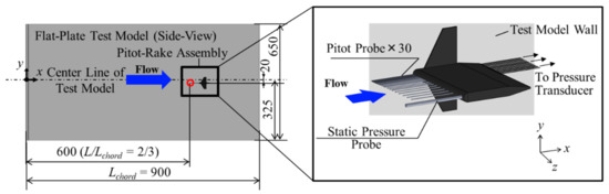
Figure 1.
Schematic illustration of flat-plate test model (left), which was installed at the center of the wind tunnel duct and pitot-rake assembly (right).
Pitot-tube measurement was done to provide reference velocities that will be used to calibrate the hot-wire signal. The reference velocities were measured for a boundary layer profile on a flat plate [10]. It should be noted that reference velocities could be measured with different ways. For example, measuring freestream velocity and relating it with hot-wire signal placed in the freestream can be used as mentioned in the Introduction. Figure 1 also illustrates a schematic of the pitot-rake assembly, which was attached to the surface of the flat-plate test model. The pitot-rake consisted of 30 probes as shown in the right figure in Figure 1. Each pitot-probe had an outer diameter of 0.5 mm, an inner diameter of 0.3 mm, and a length of 30 mm. The outside probe, which appears outside of the 30th pitot-probe, was a static pressure probe.
Totally, eight individual cases with different temperature variations were measured with respect to the velocity profile of the boundary layer by the hot-wire anemometry and the pitot-tube measurement, separately. Those datasets included a case with large temperature variation (i.e., greater than 10 °C throughout the operation duration) and a case with negligibly small temperature variation (i.e., less than 1 °C throughout the operation). Note that datasets for those eight cases were obtained as part of wind tunnel experiments for other riblet study [10]. Therefore, the aim of including those cases was to enrich datasets with various temperature variations to evaluate the applicability of the proposed method rather than considering optimized design experiment method. More details of the experiment are described in Takahashi et al. [10].
2.2. Hot-Wire Anemometry
A standard single hot-wire probe, which was made of Tungsten (KANOMAX Inc., Suita city, Osaka, Japan, 0251R-T5), was employed for the wind tunnel experiment. The probe consists of a wire, which was 2 mm long with a diameter of 5 μm and two prongs, which were 7 mm long.
The output signal from the hot-wire probe was converted to a voltage by an A/D converter (KANOMAX Inc., constant temperature hot-wire anemometer: CTA). The voltage data was recorded by a data recorder (A&D Inc., Tokyo, Japan, RM-1100) at a sampling rate of 20 kHz. At each probe position, the output voltage data was recorded for a duration of 5 s.
Figure 2 presents a schematic diagram of the measurement system with hot-wire equipment and the measurement locations on the flat-plate test model. The measurement locations were changed by changing the probe position. The vertical probe position (i.e., z-position) from the wall surface was varied from 1 to 20 mm by an electrically controlled traversing system. The x and y positions were fixed: x = 600 mm (x/xchord = 2/3) and y = −20 mm (y/ywidth = −0.031). A total of 25 measurement locations in the vertical direction was realized by changing the z position of the probe. The vertical position of the probe was changed starting from z = 1.0 to 10 mm, which corresponds to the periphery of the upper edge of the boundary layer, with an increment of 0.5 mm. Then, the vertical probe position was increased with increments of 2 mm or 4 mm until it reached z = 20 mm, expecting that the change in the velocity profile in the vertical direction at those heights would be small since the flow in this area is freestream. When reached at z = 20 mm, the probe position was changed in the opposite direction (i.e., in the order of decreasing height) in order to check for hysteresis of the detected signal and temperature dependence of the signal.
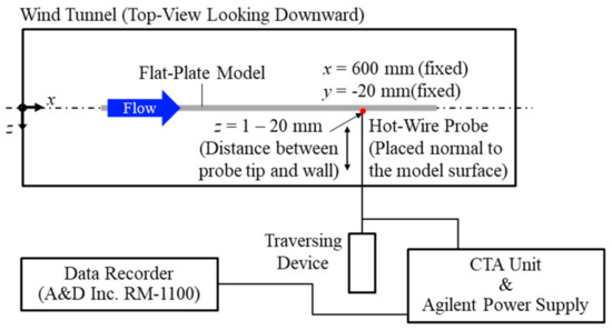
Figure 2.
Schematic diagram of hot-wire anemometry setup and measurement locations.
The probe’s soundness was confirmed at each measurement by measuring the resistance of the probe. The resistances measured before and after the testing were both around 4.0 Ω, and therefore no damage to the probe was seen. In general, an output signal detected by a tungsten-made hot-wire probe may involve a time decay under a long-duration measurement that involves a large temperature variation in the flow. It should be noted that slight time decays with temperature dependence in the output signal, which will be described in Section 2.3, were obtained during the wind tunnel experiments. However, the time decay of the output signal will also be converted to the flow velocity properly by the calibration method with the temperature correction, which will be described in detail in Section 3. The probe was also varied at each measurement.
The wire of the hot-wire probe was placed perpendicular to the flow and the probe orientation to the flow was fixed. The probe stem was also normal to the wall surface. With this configuration, the streamwise component of the flow was considered to be detected. Therefore, the measured velocity was considered as the U velocity. More details of the hot-wire anemometry applied to the same flowfield is available in Takahashi et al. [10].
2.3. Alternative Method of Temperature Correction
Figure 3 shows the freestream temperature change due to wind tunnel operation as the probe position (z) changes. The horizontal axis is the measuring number, or nondimensional operation time. The higher the measuring number, the longer the wind tunnel operation is. Temperature variations seen in four representative wind tunnel runs are presented. Obviously, the freestream temperature increased gradually as the wind-tunnel operation time increased. This observation is commonly applied to all other runs. Additionally, included are cases with relatively small temperature variations (i.e., less than 1 °C throughout the experiment), such as Run 2 in Figure 3. The temperature variation for other cases ranged from 6 to 15 °C. Thus, a variety of temperature variation ranges were considered in this study. Since the resistance of the hot-wire probe is a function of both freestream velocity and temperature, an appropriate temperature correction must be made to those wide variety of temperature variation data for quantitative analysis.
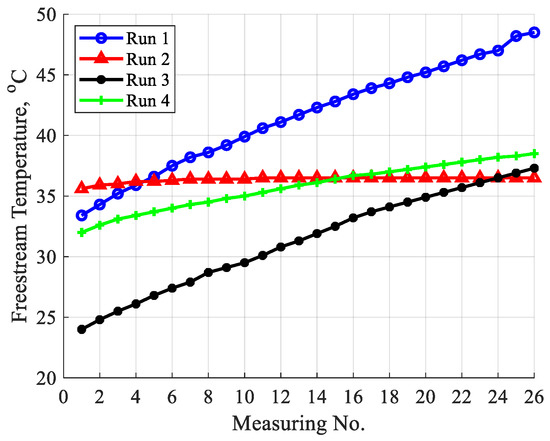
Figure 3.
Freestream temperature variation plotted against measuring number at different heights from the wall during wind tunnel operation for four different runs.
As described in the Introduction, it is necessary to know the wire temperature Tw to find the velocity by solving Equation (2), and this wire temperature is key to temperature correction for obtaining the quantitative velocity. When the true wire temperature is unknown, an alternative temperature correction with a slight modification of the original temperature correction method [8] can be used using the best-fit approach to quantitatively calibrate the velocity without knowing the wire temperature.
The functional dependence of velocity on the voltage signal (found in Equation (2)) was established by measuring velocities by the pitot-tube measurement. Freestream temperatures were also measured upon changing the probe height in the z-direction. The wire temperature (Tw) in Equation (2), which was unknown, was parametrically changed from 70 to 200 °C with an increment of 1 °C, the range of those temperatures were considered to find a possible wire temperature. Then, its value that makes the difference of the U velocity profiles obtained by the hot-wire anemometry data (Equation (2)) and the pitot-tube measurement data was sought to become zero or minimum. This iteration method is a similar but simpler method than an output error method, which has been widely applied and validated in flight control study [11,12,13], for obtaining the best fit (Equation (3)). An increment of 1 °C for Tw search was used in this study. It should be noted that the current method depends on the initial guess (e.g., 70 °C in this study) as well as the temperature increment. If the initial guess for the wire temperature is sufficiently low with small temperature increment, the optimal wire temperate can be found with better accuracy by Equation (3) but computation load may increase.
Thus, this method searches Tw values to find the minimum δtotal to facilitate the temperature correction of the voltage signal obtained from the hot-wire anemometry without knowing the actual Tw value.
3. Results
Figure 4a presents an example result for Run 1 of measured boundary layer profiles made by raw hot-wire anemometry data (HW(Raw Signal)), temperature-corrected hot-wire anemometry data (HW(Corrected)), and reference pitot-tube-measured data (Pitot). Calibrated data based on Equation (1) is also plotted for comparison denoted as HW(By Equation(1)). The nondimensional velocity normalized by the freestream velocity (in horizontal axis) is plotted against the height from the wall surface (in vertical axis). Each hot-wire data point was averaged over 5 s and the error bar shows 1σ over the averaging duration. Run 1 had the largest temperature variation (i.e., 15.1 °C) in this study. A large temperature variation during the wind tunnel operation is seen from the raw hot-wire anemometry data (HW(Raw Signal)). The temperature variance in freestream temperature, which was seen in Figure 3, became longer for longer wind tunnel operation duration. The profile calibrated by Equation (1): HW(By Equation (1)) shows large discrepancy between it and that by reference (Pitot). In this case, which had the large temperature variation, a proposed method was used instead of Equation (1). By searching for a Tw value that meets Equation (3), the hot-wire data will be corrected with regard to the temperature variance. The increment for Tw search was 1 °C as mentioned in Section 2.3. From Figure 4a, the corrected distribution (HW(Corrected)) agreed well with that obtained from the pitot-tube measurement (Pitot). The Tw for this case was found to be 111 °C with a maximum error of 1.8%.
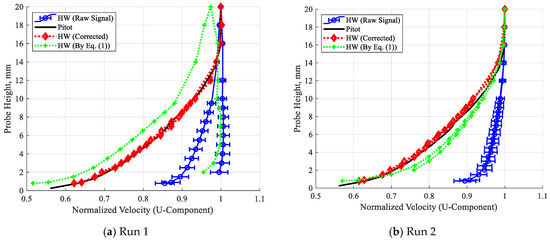
Figure 4.
Representative comparison for velocity profiles obtained by hot-wire anemometry (raw, calibrated by King’s law, and temperature-corrected by current method) and pitot-tube measurement.
Figure 4b presents an example result for Run 2 shown as Figure 4a. The temperature variation in this case was negligibly small (less than 1 °C) as seen in Figure 3. Differently from Run 1 (Figure 4a), almost no temperature variation or temperature dependence in the raw signal profile (HW (Raw Signal)) is seen. The profile calibrated by Equation (1) denoted as HW (By Equation (1)) shows better agreement with the reference profile than that of Run 1. The proposed method further improved the agreement between the temperature-corrected hot-wire data (HW (Corrected)) and reference data (Pitot). The Tw for this case was found to be 86 °C with a maximum error of 2.2%. The Tw values for other cases are also found in an appropriate range of 75 to 111 °C [8,14].
Thus, the proposed method improves the accuracy of calibration of hot-wire signal with temperature correction in case a large temperature variation exists.
Figure 5 shows the influence of the total numbers of measurement points for deriving the wire temperature. The same case as that used in Figure 4a for Run 1 is presented. At least two measurement points are needed for this evaluation. Each point contains different velocity and temperature values. All 300 combinations of 25 measurement points were compared. Obviously, the wire temperature asymptotically approached 111 °C with increasing combination number. With fewer combinations, the derived wire temperature values were dispersed.
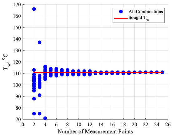
Figure 5.
Influence of total numbers of measurement points for searching the wire temperature.
To evaluate the effect of deviation of temperature, Figure 6a presents the influence of wire temperature on temperature correction. Data of Run 1 is plotted. This plot is equivalent to the calibration method using Equation (1). Various wire temperature cases are shown with their R2 factor for a linear fit. Accounting for the optimal or true wire temperature for this case (Run 1) was 111 °C, ±2 °C of deviation improved the R2 factor over 0.997. Note that applying a Tw of, for example, 108 °C to the total of 25 measurement points, the maximum error became 3.0%; and applying a Tw value of 91 °C showed an error above 10%. By allowing this temperature variation, the fewest required measurement points were found to be 7 from Figure 5. Applying ±2 °C of deviation ranges determined the error range for other cases up to 2.6%.
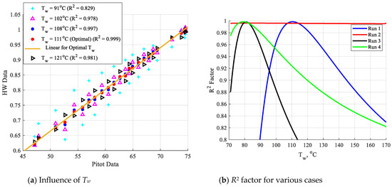
Figure 6.
Accuracy of temperature correction by various wire temperatures.
The R2 factor for various cases was plotted against Tw in Figure 6b; the other three cases were plotted as well for comparison. Similar to Run 1, Tw can be found for Run 3 and Run 4, where a large temperature variation throughout the wind tunnel operation exists as seen in Figure 3, as well. For Run 2, where a temperature variation during wind tunnel operation was small as seen in Figure 3, Tw can be found but much finer Tw search, for example, with an increment of 0.1 °C instead of 1 °C applied to other cases, was needed since the variation of R2 factor over the temperature range in search (e.g., from 70 to 170 °C in this case) was subtle.
This method can be applied to other cases as well. Figure 7 is a histogram showing uncertainties calculated as a velocity difference between the pitot-tube measurement data and the temperature-corrected hot-wire anemometry data measured at the same distance from the wall. The wire temperature for each case was the optimal temperature found by the best-fit approach proposed in this study. This uncertainty was defined by Equation (4). A total of 200 data points were obtained from eight wind tunnel runs with 25 probing at each case and were plotted. The mean and 1σ values for those error values were plotted as well. As seen in Figure 7, the mean error level was 0.48 and with 95% certainty for the error level stayed below 1.34%.
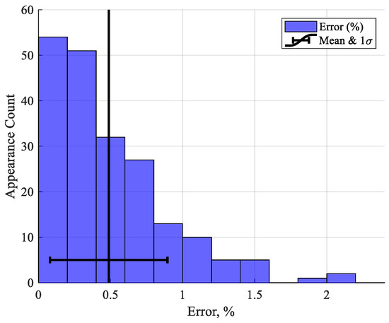
Figure 7.
Uncertainties inherent in the proposed calibration method plotted against the error of velocity calibration.
Those results indicate that the current temperature correction method that is a slight modified form of Equation (2) could be applied when reference velocities with temperatures are known regardless of the data points used for the hot-wire anemometry. Though the uncertainty level of the velocity range was found to be between 20 and 80 m/s, the proposed method on the temperature correction was validated. These results also indicate that the proposed approach could be applied regardless of velocity values and individual differences in hot-wire probes.
4. Conclusions
This study proposed a unique approach to convert a voltage signal obtained from a hot-wire anemometry to flow velocity data by making a slight modification to existing temperature-correction methods. The proposed approach is a simplified calibration method for constant-temperature hot-wire anemometry without knowing exact wire temperature. Other than the hot-wire signals, the necessary data are the freestream temperature and a set of known velocities that gives reference velocities obtained from the pitot-tube measurement. The proposed approach was applied to various boundary layer profiles with large temperature variations while the wire temperature was unknown. By using a best-fit approach between the velocities in the boundary layer obtained by hot-wire anemometry and by the pitot-tube measurement, which provides reference data, the unknown wire temperature was sought. The proposed approach was confirmed to be applicable to a velocity range between 20 and 80 m/s and with temperature variations up to 15 °C with an uncertainty level of 2.6% at most for the current datasets. Thus, the proposed approach could be used as a simplified calibration method for the constant-temperature hot-wire anemometry without knowing the wire temperature in case large temperature variations exist.
Author Contributions
H.T. is responsible for the entire work from data acquisition at wind tunnel experiments, conceptualization, establishing methodology, data analysis, and writing the original manuscript entirely; M.K. managed the overall project and reviewed; H.I. and S.K. worked on data acquisition at wind tunnel experiments. All authors have read and agreed to the published version of the manuscript.
Funding
This research received no external funding.
Acknowledgments
This study was conducted as part of the Flight Investigation of Skin-Friction Reduction Eco-Coating (FINE) project led by JAXA Aeronautical Technology Directorate. The authors wish to thank the aerodynamics research unit and Tomonari Hirotani at the JAXA Aeronautical Technology Directorate for assistance with the wind tunnel experiment, and Akira Nishizawa for help with the hot-wire anemometry. The authors also acknowledge Masato Asai and Ayumi Inazawa at Tokyo Metropolitan University, Shihoko Endo and Kaoru Iwamoto at the Tokyo University of Agriculture and Technology, and Ryoko Shinohara at O-WELL corporation for their support regarding riblet design and its fabrication.
Conflicts of Interest
The authors declare no conflict of interest.
Nomenclature
| a, b | constant coefficient |
| E | voltage, V |
| H | probe height, mm |
| k | thermal conductivity, W/(m⋅K) |
| T | temperature, °C |
| U | streamwise velocity component (U velocity), m/s |
| x | streamwise coordinate |
| y | spanwise coordinate |
| z | vertical coordinate |
| δ | difference |
| ν | kinematic viscosity, m2/s |
| σ | standard deviation |
| Subscripts | |
| a | freestream (air) |
| HW | hot-wire |
| i | index number |
| pitot | pitot-tube measurement |
| total | total value |
| w | wire |
References
- Stainback, P.C.; Nagabushana, K.A. Review of Hot-Wire Anemometry Techniques and the Range of Their Applicability for Various Flows. Electron. J. Fluids Eng. Trans. Am. Soc. Mech. Eng. 1997, 119, 1–54. [Google Scholar]
- Sakaue, S.; Kamata, M.; Arai, T. Turbulent Intensity in Supersonic Mixing Transition by Streamwise Vortices -Fluctuation Measurements by Hot-Wire Anemometer and PIV-. Trans. JSASS Aerosp. Technol. 2020, 18, 258–265. [Google Scholar]
- Duri, D.; Baudet, C.; Moro, J.-P.; Roche, P.E.; Diribarne, P. Hot-Wire Anemometry for Superfluid Turbulent Coflows. Rev. Sci. Instrum. 2015, 86, 025007. [Google Scholar] [CrossRef] [PubMed]
- Souza, F.; Tavoularis, S. Hot-Wire Responses in Compressible Subsonic Flow. AIAA J. 2020, 58, 3332–3338. [Google Scholar] [CrossRef]
- Massouh, F.; Dobrev, I. Exploration of the Vortex Wake behind of Wind Turbine Rotor. J. Phys. Conf. Ser. 2007, 75, 012036. [Google Scholar] [CrossRef]
- King, L.B. On the Convection of Heat From Small Cylinders in a Stream of Fluid: Determination of the Convection Constants of Small Platinum Wires, with Applications to Hot-Wire Anemometry. Philos. Trans. R. Soc. Lond. 1914, 214, 373–432. [Google Scholar]
- Bourget, P.-L. Calibration Method for A Hot Wire Anemometer. J. Phys. E Instrum. 1976, 9, 353–358. [Google Scholar] [CrossRef]
- Hultmark, M.; Smits, A.J. Temperature Corrections for Constant Temperature and Constant Current Hot-Wire Anemometers. Meas. Sci. Technol. 2010, 21, 105404. [Google Scholar] [CrossRef]
- Kannuluik, W.G.; Carman, E.H. The Temperature Dependence of the Thermal Conductivity of Air. Aust. J. Sci. Res. Ser. A Phys. Sci. 1951, 4, 305–314. [Google Scholar]
- Takahashi, H.; Iijima, H.; Kurita, M.; Koga, S. Evaluation of Skin Friction Drag Reduction in the Turbulent Boundary Layer Using Riblets. Appl. Sci. 2019, 9, 5199. [Google Scholar] [CrossRef]
- Lichota, P. Inclusion of the D-optimality in multisine manoeuvre design for aircraft parameter estimation. J. Theor. Appl. Mech. 2016, 54, 87–98. [Google Scholar] [CrossRef]
- Dul, F.; Lichota, P.; Rusowicz, A. Generalized Linear Quadratic Control for a Full Tracking Problem in Aviation. Sensors 2020, 20, 2955. [Google Scholar] [CrossRef] [PubMed]
- Gautier, M.; Janot, A.; Vandanjon, P. A New Closed-Loop Output Error Method for Parameter Identification of Robot Dynamics. IEEE Trans. Control. Syst. Technol. 2013, 21, 428–444. [Google Scholar] [CrossRef]
- Abdel-Rahman, A.A.; Tropea, C.; Slawson, P.; Strong, A. On Temperature Compensation in Hot-Wire Anemometry. J. Phys. E Sci. Instrum. 2000, 20, 315–319. [Google Scholar] [CrossRef]


Publisher’s Note: MDPI stays neutral with regard to jurisdictional claims in published maps and institutional affiliations. |
© 2020 by the authors. Licensee MDPI, Basel, Switzerland. This article is an open access article distributed under the terms and conditions of the Creative Commons Attribution (CC BY) license (http://creativecommons.org/licenses/by/4.0/).