Article

Metaheuristics and Support Vector Data Description for Fault Detection in Industrial Processes

by
Jesús Alejandro Navarro-Acosta
1,
Irma D. García-Calvillo
1,
Vanesa Avalos-Gaytán
1 and
Edgar O. Reséndiz-Flores
2,*
1
Research Center on Applied Mathematics, Autonomous University of Coahuila, Prolongación David Berlanga, Edificio S, Primer Piso, Camporredondo, Saltillo 25115, Mexico
2
Division of Postgraduate Studies and Research, Tecnológico Nacional de México/IT de Saltillo. Blvd. Venustiano Carranza 2400, Colonia Tecnológico, Saltillo 25280, Mexico
*
Author to whom correspondence should be addressed.
Appl. Sci. 2020, 10(24), 9145; https://doi.org/10.3390/app10249145
Submission received: 28 November 2020 / Revised: 11 December 2020 / Accepted: 16 December 2020 / Published: 21 December 2020
(This article belongs to the Section Computing and Artificial Intelligence)

Abstract

:
In this study, a system for faults detection using a combination of Support Vector Data Description (SVDD) with metaheuristic algorithms is presented. The presented approach is applied to a real industrial process where the set of measured faults is scarce. The original contribution in this work is the industrial context of application and the comparison of swarm intelligence algorithms to optimize the SVDD hyper-parameters. Four recent metaheuristics are compared hereby to solve the corresponding optimization problem in an efficient manner. These optimization techniques are then implemented for fault detection in a multivariate industrial process with non-balanced data. The obtained numerical results seem to be promising when the considered optimization techniques are combined with SVDD. In particular, the Spotted Hyena algorithm outperforms other metaheuristics reaching values of F1 score near 100% in fault detection.

1. Introduction

Currently, machine learning and nature-inspired algorithms are being applied in several research fields to obtain optimal results. Some real applications include medical diagnosis based on the patient’s symptoms [1], fraud detection in economic transactions [2], identification of patterns of investment in order to buy/sell in a more efficient manner [3], image detection to predict city traffic, machine failure and the design of autonomous vehicles, among others [4]. There are some previous studies regarding fault detection and fault diagnosis based on Dynamic Weight Principal Component Analysis (PCA) [5], Principal polynomial analysis [6], PCA and a Bayesian network [7], deep convolutional neural network [8], Hidden Markov Model and Bayesian Network [9], among others. However, statistical assumptions about the distribution of the process data should be made in some of these approaches. Support Vector Data Description (SVDD) [10] and Artificial Neural Networks (ANN) algorithms share the same concept using the linear learning model for pattern recognition. ANN tries to converge to a local minimum using the gradient descent learning algorithm and suffers from overfitting problems. On the other hand, SVDD tends to find a global solution during training since the complexity of the model has been taken into account as a structural risk in SVDD formation. ANN minimizes only empirical risk learned from training samples and SVDD considers not only the empirical risk but the structure risk. Thus, SVDD training results show better generalization capability than those obtained with ANN.
In industry, machine learning classifiers are implemented to focus on faults detection. In [11,12], reviews of machine learning applications in the manufacturing industry are presented. The use of artificial neural networks in the modeling and optimization of processes is emphasized as well as the application of SVM for quality assessment in industries. Another application of SVM for the early failure prediction in the oil and gas industry is shown in [13]. In [14], a monitoring platform using Artificial Neural Network and the Support Vector Machine is proposed and applied to the prediction of the performance of aeronautical engines and health diagnosis. Nevertheless, conventional algorithms are also created to perform two-class or multi-class classification tasks. Because of this, data containing all class of information on the processes are required. Recently, machine learning algorithms have been used in fault detection, but there is sometimes the downside of having more information available from one of the kind. For example, if a relatively new machine is in operation, it is very likely that only the data corresponding to normal operation are available. In this study, a method for fault detection is proposed which is able to deal with processes or machines where observations or data about the faults are scarce for the training phase by using the one class classifier known as Support Vector Data Description (SVDD) [10]. The choice of hyper-parameters is one of the most important features for SVDD. These parameters are associated with the hyper-sphere as well as with the kernel function chosen for the classification. In this study, these hyper-parameters are simultaneously optimized using metaheuristic techniques. Furthermore, a comparison among four optimization techniques is reported in order to evaluate the quality of the obtained results. The results are satisfactory when applied to a process of fault detection at low computational cost.
There are some studies covering different SVDD algorithm applications [15,16,17]—most of them optimizing the hyper-parameters using approaches like grid search, which is computationally expensive. To obtain these parameters in a more efficient manner, some authors have considered metaheuristic algorithms. Particle swarm optimization (PSO) and genetic algorithms can be often found in literature. Ref. [18] presents a brief general description about hyper-parameter optimization in Support Vector Machines (SVM). In this context, the ant colony algorithm is chosen in [19] for feature selection and parameter optimization in SVM for fault diagnosis. Ref. [20] used genetic algorithms to optimize parameters corresponding to the kernel function. Optimization of the hyper-sphere parameters together with those associated with the Gaussian radial base kernel function are studied by [21] using grid search. Ref. [22] obtained optimal results by the combination of grid search and PSO.
In the last few decades, researchers have developed several nature-inspired optimization algorithms that mimic some biological behaviors or physical phenomena. Techniques based on swarm intelligence mimic the socially intelligent behavior of groups of species. Search algorithms start with a group of randomly generated solutions generally naming a population evolving throughout successive generations and promote the population improvement throughout the iterations. In this study, a performance comparison is presented corresponding to four of these metaheuristics for calculation of the hyper-parameters. Besides PSO, which has been widely used for these purposes, the considered algorithms in this study have demonstrated their efficiency in solving optimization problems applied to engineering. Furthermore, the performance is tested for the Spotted Hyena Optimization (SHO) algorithm, Krill herd (KH) algorithm, and Squirrel Search Algorithm (SSA).
The SHO is a recent metaheuristic based on swarms which mimics the social behavior of these animals in nature. Among the vast amount of metaheuristics, SHO has shown great advantages in the exploration of diverse search spaces compared to other state-of-the-art approaches [23]. SHO has been implemented to solve a wide range of engineering problems like prediction of materials resistance during cutting processes [24]. SHO is used in combination with neural networks to improve the prediction ability of these algorithms. In [25], two complex engineering problems with restrictions like the design of bar armor and the design of multiple disk clutch brakes are solved. The results show the efficiency of SHO in solving these problems compared to other optimization algorithms like PSO and ACO. It showed its applicability in environments of a high dimension with a low computational cost. Ref. [26] implements SHO for design optimization in aerodynamic surface and optical buffer problems where the obtained numerical results are then compared with algorithms like Grey Wolf Optimizer, Genetic Algorithm, and PSO, among others. Likewise, the binary version of SHO has been developed and used to build wrapping approaches for feature selection in different sets of UCI data [27]. Moreover, SHO has been hybridized with other algorithms like PSO to improve its abilities to solve various engineering problems [28]. Recently, Ref. [29] implements an SHO version able to deal with multi-objective problems for the prediction of characteristics in gene selection through its combination with machine learning algorithms like SVM.
The KH algorithm is a recent nature-based algorithm inspired by the individual krill herding behavior. This algorithm was introduced in [30]. The KH algorithm works to achieve the minimum distance between individual krill and the nearest food. This algorithm has been successfully used in solving many problems of numerical optimization, electric and power system problems, text grouping, breast cancer detection, and the training of neural networks [31,32,33]. More recently, the possibility of applying this algorithm for the grouping of text documents is studied in [34], while the same problem is addressed in [35] using a hybrid algorithm based on KH. The grouping based on the KH algorithm is proposed in [36] for the network of wireless sensors. A method for diagnosing bearing failure based on KH and a kernel extreme learning machine is proposed in [37]. An improvement of KH applied to fault diagnosis with a Support Vector Machine to solve the power transformers’ fault diagnosis problem based on the analysis of dispersed gases is presented in [38].
The SSA is a metaheuristic approach based on the behavior of flying squirrels which are a diversified nocturnal tree rodent group that are highly adjusted to gliding locomotion. The SSA mimics the dynamic food search behavior of flying squirrels and their effective form of locomotion, known as gliding, which is a very effective mechanism for traveling long distances. The algorithm has been recently proposed [39,40]. Moreover, it has proven its good performance in some applications, for example in [41], is applied for the optimization of a backpropagation artificial neural network (BPNN) using a multi-objective method based on SSA to optimize the main parameters of a continuous galvanization process for advanced DP Steels. In [42], SSA is used to optimize a complex problem where combined heat and energy distribution for various regions is modeled integrating renewable energy sources. In [43], a hybrid algorithm based on the combination of SSA and the optimization of invasive weed is proposed. This algorithm is combined with the Support Vector Machine and the deterministic maximum likelihood algorithm to perform the classification of air quality levels. Recently, a Chaotic SSA variant for optimum programming of multiple tasks in an infrastructure cloud environment as service is reported in [44].
The main contribution of this paper consists of a fault detection system using a combination of SVDD with some optimization methods like SHO, KH, SSA, and the well-known PSO. The effectiveness of the used different meteheuristics, for the parameters optimization corresponding to the hyper-sphere as well as those associated with the Gaussian radial basis kernel used in SVDD, is compared. As it will be shown, promising results are obtained when the mentioned swarm intelligence algorithms are combined with SVDD and applied to fault detection in a real industrial problem.
The rest of the paper is organized as follows: theoretical background is presented in Section 2, the proposed methodology for fault detection is described in Section 3, and this is followed by the industrial application section and finally some conclusions and future work are discussed in the last section.

2. Theoretical Background

2.1. Support Vector Data Description

Tax and Duin [10] proposed the SVDD classification method which determines a close boundary around the data set for a given class: a hyper-sphere characterized by a center and a radius R 0 that defines a separation between the inner region with high data density and the outer region with low density. The data that lie right at the limit of the hyper-sphere are called the support vectors while those outside are the outliers. Let { x i : i = 1 , 2 , 3 , , N } be a column vector set and x 2 = x · x the training set for which a description must be specified and assume that x i ’s show variances in all given directions. The data set delimitation of the inner region of the hyper-sphere will be minimized with an error function which minimizes the possibility of accepting outliers and such a function is defined as:
min F ( R , a , ξ i ) = R 2 + C i ξ i s . t . x i a 2 R 2 + ξ i , ξ i 0 i
where ξ i are the slack variables that will penalize the largest distances, and C is a control parameter of the trade-off between volume of the hyper-sphere and the errors [45]. Applying the Lagrange multipliers method, the following equations arise:
L ( R , a , α i , γ i , ξ i ) = R 2 + C i ξ i α i R 2 + ξ i x i 2 2 a · x i + a 2 i γ i ξ i
with α i 0 as Lagrangian multipliers and γ i > 0 .
The dual formulation of the equations in (2) can be obtained by solving the KKT conditions, which reads
min i α i x i , x i i j α i α j x i , x j s . t . 0 α C
In case a given x i satisfies x i a 2 < R 2 + ξ i , then α i = 0 ; otherwise, when x i satisfies x i a 2 = R 2 + ξ i , the corresponding Lagrange multiplier α i is strictly greater than zero.
The vectors x i corresponding to α i > 0 represent the set of vectors necessary to characterize a set of data, and this set of vectors can be called support vectors of the description [46]. When there is a new vector z , the distance to the center of the sphere can be computed. If this distance is smaller than R, z is accepted as a new vector in the description of the data, that is,
z a 2 = z · z 2 i = 1 l α i z · x i + i = 1 l j = 1 l α i α j x i · x j R 2
Note that, if the inner product in Equation (1) is replaced with a kernel function K x i , x i a description for nonlinear data sets can then be obtained. In this manner, data are mapped to a higher dimension feature space by means of the kernel function, and this makes the nonlinear data separable [47]. Thus, the problem can be reformulated as follows:
min i α i K x i , x i i j α i α j K x i , x j s . t . 0 α C
where α i remains as the Lagrange multipliers and K x i , x j is a kernel function used as a functional mapping.

2.2. Spotted Hyena Optimizer (SHO)

Proposed by Dhiman and Kumar [48], SHO is a recent optimization technique that mimics the behavior of spotted hyenas when hunting. Spotted hyenas are social animals, and they hunt for prey by means of trusted friends groups and through their great ability to recognize their prey. These groups can be of up to 100 hyenas, and this is why the hunting method tends to be very effective and gets results in short periods of time. The main stages of this algorithm include searching, surrounding, and attacking the prey, in addition to other spotted hyena-seeking behaviors. In SHO, there is a search agent leader, and it is assumed that it knows the location of the prey. In this way, the other agents update their position to form friend groups around the leader. Next, the mathematical models corresponding to the mentioned several stages of this algorithm are described.

2.2.1. Encircling Prey

In this stage, the best current potential solution is considered like the prey. In that way, the other hyenas update their position around it. The mathematical model corresponding to this behavior is as follows:
D h = B · P p ( x ) P ( x )
P ( x + 1 ) = P p ( x ) E · D h
where D h determines the distance between the prey and the hyena, x shows the current iteration, B , and E are the coefficient vectors. P p is the position vector of the prey while P is the position vector of the spotted hyena. The vectors B and E are calculated as follows:
B = 2 · r d 1
E = 2 h · r d 2 h
h = 5 ( iteration ( 5 / max i t e r a t i o n ) )
where h decreases linearly from 5 to 0 in the course of the highest number of iterations. r d 1 and r d 2 are random vectors in [ 0 , 1 ] .

2.2.2. Hunting

Given that spotted hyenas hunt in “trusted friend” groups, the searching agents must form conglomerates around the best agent. The following equations model such behavior,
D h = B · P h P k
P k = P h E · D h
C h = P k + P k + 1 + + P k + N
where P h defines the position of the first best hyena, P k shows the position of the rest of the hyenas, and N refers to the number of hyenas calculated as follows:
N = Count n o s P h , P h + 1 , . . . , ( P h + M )
similarly, M is a random vector in [ 0 , 1 ] .

2.2.3. Attacking the Prey

The mathematical formulation for attacking the prey reads
P ( x + 1 ) = C h N
where P ( x + 1 ) saves the best solution and updates the positions of other searching agents according to the position of the best searching agent.

2.2.4. Searching for Prey (Exploration)

The vector B previously defined provides random values for the exploration during all iterations. Therefore, this mechanism effectively allows for avoiding local optima even in the final iterations.

2.3. Krill Herd Algorithm (KH)

The KH algorithm is inspired by the simulation of small crustaceans (Krill) behavior which live underwater. These crustaceans have the ability to form large swarms to avoid predators. The fitness function in the KH algorithm used to solve global optimization problems is based on the density of the swarm and the location of the food. Each krill migrates toward the area of highest density and at the same time continues to search for the places that contain the most food. Increasing density and foraging are used as a means to bring krill to global optimum levels at the end.
During the moving process, each krill moves towards the best option based on three essential movements:
(i)
movement generated by other krill;
(ii)
food search activity;
(iii)
physical diffusion.
The equation describing the krill moving process is as follows:
d X i d t = N i + F i + D i ,
where N i is the motion produced by other krill, F i is the food search motion, and D i is the random diffusion of the ith krill individual.
The direction of induced motion α i is decided by the following parts: target effect, local effect, and a repulsive effect. For a krill individual, this movement can be defined as
N i n e w = N max α i + ω n N i o l d
where N i n e w , ω n , and N i o l d denote the maximum induced speed, the inertia weight, and the last motion, respectively.
The food searching motion is influenced by two components: the food location and the previous experience about food location. For the ith krill, this motion can be expressed as follows:
F i = V f β i + ω f F i o l d
where V i is the feeding speed, ω f is the inertia weight, F i o l d is the last feeding motion, and
β i = β i f o o d + β i b e s t
The physical diffusion is essentially a random process. This motion can be computed based on a maximum diffusion speed D max and a random directional vector δ as follows:
D i = D max δ
The position in KH from t to t + Δ t is given by the following equation:
X i ( t + Δ t ) = X i ( t ) + Δ t d X i d t
The interested reader is referred to [30] for more detailed information about the KH algorithm.

2.4. Squirrel Search Algorithm SSA

Recently, Ref. [39] proposed an innovative nature-inspired algorithm for optimization, the Squirrel Search Algorithm, which has been very efficient in solving unconstrained numerical optimization problems. The algorithm mimics the strategies of flying squirrels in searching for food sources and escaping predators. A summer and winter phases are considered since the motion dynamics are different depending on the season. This strategy allows it to escape from local minima, thus raising the likelihood of reaching the global optimum. The algorithm considers a certain number of flying squirrels in a forest. It is assumed that each squirrel is located on a tree. Each squirrel searches for food by gliding among trees looking for the best food source and there are three types of trees: normal tree (no food), oak tree (acorn nuts food source), and hickory tree (hickory nuts food source). It is supposed that there is a population of N flying squirrels in the forest, one at hickory tree, N f s at acorn trees, and the rest ( 1 N f s N ) at normal trees. Each squirrel is represented by a vector with D components corresponding to the dimension of the problem. Initially, the flying squirrels are in a random position to start the algorithm and the location of the squirrels can be represented by the following expression:
F S i = F S L + r a n d ( 1 , D ) × ( F S U F S L )
Since each row represents one squirrel, this matrix can be initialized in a random manner with a uniform distribution between ( 0 , 1 ) with the lower and upper dimensions of each squirrel as F S U and F S L , respectively. Considering the full matrix, then the fitness evaluation corresponding to the location for each squirrel gives a fitness vector with the value of the objective function. This vector is arranged in ascending order in order to identify the best value associated with the best food source (hickory tree F h ), another food source (acorn tree F a ), and the squirrels in normal trees F n , in such a manner that each squirrel can be identified.
Considering the case when foraging squirrels do not run into a predator, flying squirrels then look for better food sources in the forest, which implies that F h remains unchanged. The destination of F a is F h and the destination of F n is random between F a or F h . In the case when they find a predator, they are forced to seek and find shelter in a random location. Their behavior can be mathematically described as follows:
Case 1. The flying squirrels in acorn trees move to hickory trees, according to the following equation:
F S i t + 1 = F S i t + d g × G c × ( F h t F S i t ) if r P d p random   location , otherwise
Case 2. Some of the flying squirrels on normal trees move to the acorn trees looking for better food and some that have already been fed move to hickory trees in order to store food. The new locations read:
F S i t + 1 = F S i t + d g × G c × ( F a t F S i t ) if r P d p random   location otherwise
where r ( 0 , 1 ) is a random number, P d p represents the predator appearance probability, t is the current iteration, G c a constant, and d g is the gliding distance. The detailed calculation of these parameters are introduced in [39].
The season changes that help the algorithm to escape from local optima are considered by calculating the season constant as follows:
S c t = k = 1 D ( F a i , k t F h , k t ) 2 i = 1 , 2 , , N f s
S min = 10 e 6 ( 365 ) t / ( T / 2.5 )
where T is the maximum number of iterations and c is the current iteration. Moreover, the condition is verified if S c t < S min . If this happens, the flying squirrels are relocated according to the following equation:
F S i t + 1 = F S L + Lévy ( n ) × ( F S U F S L )
All parameters suggested in [39] have been used.

2.5. Particle Swarm Optimization

Particle Swarm Optimization (PSO) is a population search algorithm based on the simulation of the social behavior of birds, bees, or a school of fishes [49]. In this stochastic search technique, a multidimensional vector represents a particle in a multidimensional search space. These particles move toward the next position depending on the velocity vector associated with them. The velocity is updated based on the current velocity and the best position it has explored so far. This algorithm used the global best solution concept to obtain the optimal solution. At each iteration, the global best solution is recorded and updated [50].
Let y i = ( y i 1 , y i 2 , . . . , y i d ) t be the i-th particle of the swarm in a d-dimensional search space with a corresponding velocity v i = ( v i 1 , v i 2 , . . . , v i d ) t . Thus, the equations that conduct the particle’s movements read
v i ( t + 1 ) = w v i ( t ) + c 1 ϕ 1 ( p i b e s t y i ( t ) ) + c 2 ϕ 2 ( p g b e s t y i ( t ) ) y i ( t + 1 ) = y i ( t ) + v i ( t + 1 )
where c 1 and c 2 are acceleration coefficients, and ϕ 1 and ϕ 2 are random variables with uniform distribution in [ 0 , 1 ] . p i b e s t and p g b e s t are the best local and global particle positions so far, respectively. w denotes the inertia weight which shows the effect of previous velocity vector on the new vector.

3. Methodology for Fault Detection

The methodology presented in this study consists of pre-processing of data, that is, cleaning and structuring data to obtain a matrix of m observations with n process variables. Once this is done, the different metaheuristics are implemented to optimize the training of a one-class classifier (SVDD), that is, the hyper-parameters are optimally found that improve the abilities of SVDD for faults detection in industrial processes where there is not much faulty information available. In particular, advantages of the exploration and exploitation of metaheuristic algorithms are taken in order to tune the hyper-parameters C in SVDD and s for the RBF kernel (16). Once the SVDD training is optimized, it will be ready to monitor new data and detect possible faults in the multivariate industrial process. Figure 1 shows the process of the described methodology:
K ( x i , x j ) = e x p x i x j 2 / 2 s 2
With the purpose of performance comparison during the optimization and training processes of SVDD, some metaheuristic algorithms such as SHO, KH, SSA, and PSO are implemented which show great efficiency in solving engineering problems. Thus, four approaches arise and need to be compared, that is: (1) SHO-SVDD, (2) KH-SVDD, (3) SSA-SVDD, and (4) PSO-SVDD. The metric under consideration is the well known F1 score (17) due to the fact that this metric takes into account precision and sensitivity. Such metric is computed based on the true and false positives (TP and FP) and negatives (TN and FN) (18) and (19). Moreover, this is highly relevant in the detection of faults in industrial processes. The F1 score value is found between 0 and 1, that is, a value of 1 means that the algorithm can detect the faults without errors. In this sense, the possible solutions generated by the different metaheuristics (particles, group of hyenas, etc.) for both hyper-parameters (C and s) are used in the training and testing phases of SVDD yielding several values of F1 score. Therefore, the different metaheuristics will adjust their solutions through the iterations in order to maximize the F1 score value:
F 1 score = 2 · Re · Pr Re + Pr
Pr = TP TP + FP
Re = TP TP + FN

4. Industrial Application

The four approaches described above are applied to the injection moulding process of car pedals in a local automotive industry. The implementation is carry out in a plastic injection machine with the capability to produce four pieces per cycle and save the relevant information in each run i.e., the parameters used to produce such pieces are automatically stored in a database. Subsequently, the pieces are classified as good or bad through several quality tests carry out by the technical staff. The injection moulding process involves 36 variables listed in Table 1. This data set was selected by the expert personnel of the process and consists of variables of diverse nature like temperatures, pressure, time, etc., corresponding to several machine operational features such as heating power, mold position, and injection time. Since this machine just recently started operating, the primary data provided by the company include 154 observations of normal operation mode. Once the data are cleaned up and structured, the training of the one-class classifier takes place. As soon as the algorithm is trained in order to determine the system’s capability, 64 new observations provided by the company are tested. This new data set includes observations corresponding to machine faults, that is, measurements where the injection process does not meet the quality standards. Then, the F1 score metric is calculated and the metaheuristics tune the SVDD hyper-parameters in order to achieve a better F1 score.
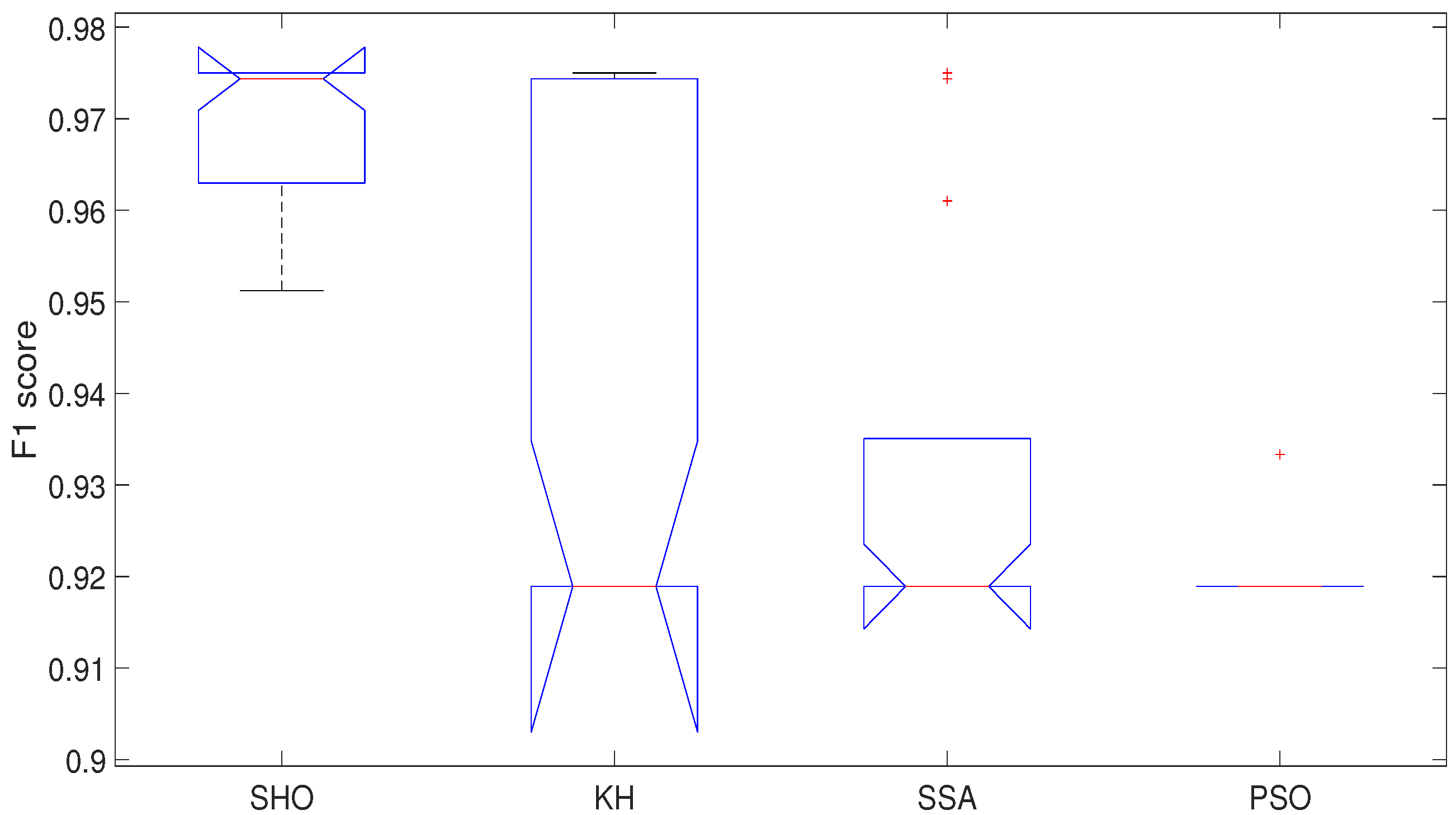
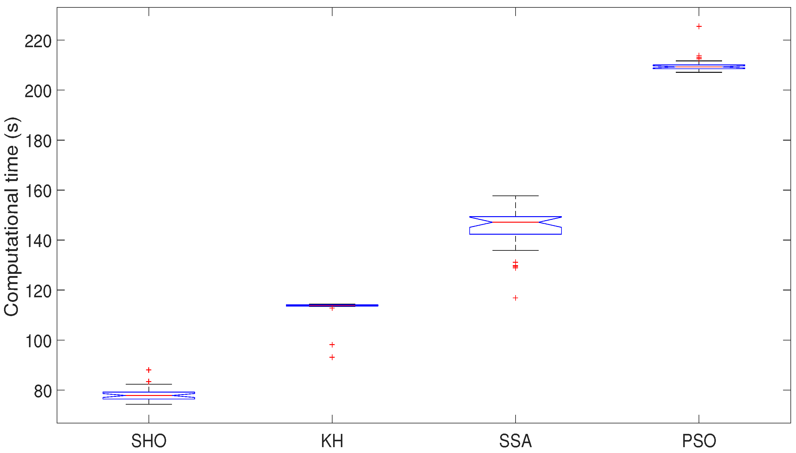
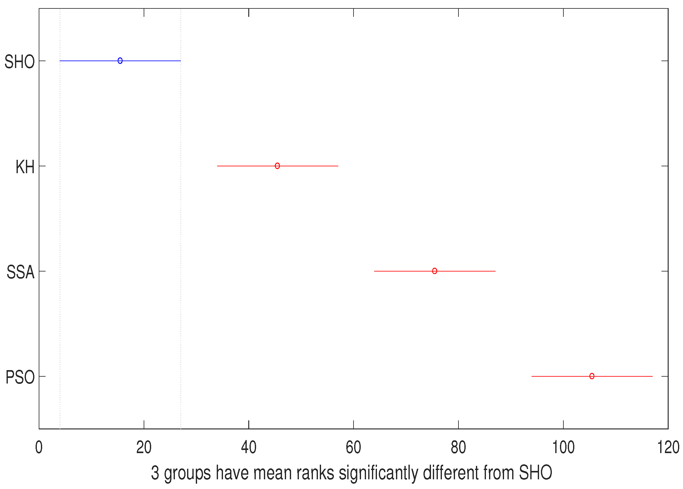
The parameters of the different metaheuristics were selected according to their authors and the corresponding values are specified in Table 2. The number of iterations was selected in experimental testing where it was determined as the maximum amount of iterations that produced changes in the results. The search range is from 0.001 to 600 for the hyper-parameters. Table 3 shows the different values and descriptive statistics of the F1 score metric and the computational times corresponding to 30 runs using each of the four approaches. As it can be seen, the SHO algorithm reaches the highest mean value of F1 score (0.9702) with a small variability i.e., standard deviation (std) equal to 0.0074. Furthermore, this approach presents the highest F1 score values in 80% of the experiments while SSA, KH, and PSO achieve similar performance only in 16, 13, and 0%, respectively. On the other hand, SHO presents the least computational time in the 100% of the runs achieving execution times two and even three times less than SSA and PSO. In addition, SHO presents the minimum variability with respect to the remaining approaches. In order to confirm the statistical significance of the results, a Mardia test is first performed to determine if the data present multivariate normal distribution. Since the data set is not normally distributed, the non-parametric ANOVA test of the Kruskal–Wallis is used. Figure 2 and Figure 3 show the corresponding box plots for the implemented approaches. As it can be seen in Figure 2, SHO reaches the highest median F1 score value with low variability. On the other hand, the remaining approaches present the equal median F1 score values. However, KH shows the highest variability on its results. Although SSA sometimes yields similar results than those of SHO, they are so sporadic throughout the runs which is the reason for the boxplot to show these values as outliers. Figure 3 clearly depicts that SHO achieves the best computational times since the highest outliers of SHO are below of the lowest valued reported by KH. Table 4 and Table 5 present the numerical results of the ANOVA test where for both cases (F1 score and computational time) the p-value is much lower than the significance level of 0.05. Thus, there is a statistical significance of the difference between the means of the results obtained by the four approaches. On the other hand, the high error in the sum of the squares (SS) in the F1 score analysis shows that there is a great variability which can not be explained by the predictors. Once considerable differences have been detected when using the Kruskal–Wallis ANOVA, a post hoc Tukey test is performed to determine the mean with the most significant difference. This analysis compares the means of all treatments with the mean of every other treatment and the best available method is considered in cases when confidence intervals are desired (for details, refer to [51]). Figure 4 and Figure 5 show the graph of the estimates and comparison interval. Each group mean is represented by a little circle and the interval is represented by a line extending out from the circle. Two group means are significantly different if their intervals are disjoint and they are not significantly different if their intervals overlap. As it can be seen, the SHO approach does not overlap with any other in both cases (F1 score and computational times), i.e., the Tukey test concludes that there is a significant difference between the SHO algorithm and the remaining approaches. This shows that SHO-SVDD offers a higher performance for fault detection in the plastic injection machine (F1 score is equal to 0.9702 in average) with a shorter computational training time. Finally, the overfitting effect is analyzed to test the SHO-SVDD generalization performance. The complete data set (normal and mixed operation samples) is used to implement a K-fold cross validation procedure. In addition, 5-fold (test 1) and 10-fold (test 2) cross validation are computed 30 times, and F1 score mean value is calculated i.e., a total of 150 and 300 training-test experiments are computed, respectively. The obtained F1 score mean values are 0.9701 for test 1 and 0.9714 for test 2, both are very close to F1 score mean value of 0.9702 obtained in the previous analysis. Considering this, it is concluded that the SHO-SVDD approach for fault detection presents a good generalization for this particular data set.

5. Conclusions and Future Work

In this paper, a methodology for fault detection in multivariate processes is presented. This proposal is able to work in industrial processes and machines which are recently operated. It can deal with little data about faults by the implementation of a one class classifier (SVDD). Such algorithm is optimized during its training stage, that is, its hyper-parameters are tuned using a recent metaheuristic based on the behavior of spotted hyenas (SHO). In order to evaluate its computational performance, SHO has been compared with three other metaheuristics (KH, SSA y PSO) that have been successfully implemented for solving several engineering problems. The approaches were tested using data taking from a plastic injecting machine in the automotive industry. The results after 30 runs show that SHO reaches higher values in the F1 score metric, that is, it shows higher performance for fault detection in considerably shorter computing time with respect to the rest of the considered approaches. Furthermore, a non-parametric statistical analysis was performed to prove the statistical significance of the superior performance of SHO. The Kruskal–Wallis test and the post hoc analysis show that there is a significant statistical difference between SHO and the other metaheuristics. Moreover, SHO-SVDD was tested for generalization performance using 5-fold and 10-fold cross validation. The obtained F1 score mean values were 0.9701 and 0.9714, respectively, which are very close to the F1 score mean value of 0.9702 obtained by the proposed analysis. Considering this, it is concluded that the SHO-SVDD method presents a good generalization to classify this data set. Based on this, the SHO-SVDD approach seems to be the best to carry out fault detection for this particular industrial application. As future work, some feature selection approaches will be implemented to obtain a subset of variables that allows for performing a fault diagnosis in order to trace back operational issues or other problems in the process.

Author Contributions

Conceptualization, J.A.N.-A. and I.D.G.-C.; Data curation, E.O.R.-F.; Formal analysis, E.O.R.-F.; Investigation, J.A.N.-A., I.D.G.-C. and V.A.-G.; Methodology, J.A.N.-A. and I.D.G.-C.; Project administration, J.A.N.-A., I.D.G.-C., V.A.-G. and E.O.R.-F.; Resources, J.A.N.-A., I.D.G.-C., V.A.-G. and E.O.R.-F.; Software, J.A.N.-A. and I.D.G.-C.; Supervision, J.A.N.-A., I.D.G.-C. and E.O.R.-F.; Validation, J.A.N.-A. and I.D.G.-C.; Visualization, J.A.N.-A. and V.A.-G.; Writing—original draft, J.A.N.-A., I.D.G.-C., V.A.-G. and E.O.R.-F.; Writing—review & editing, V.A.-G. and E.O.R.-F. All authors have read and agreed to the published version of the manuscript.

Funding

This research was funded by the Autonomous University of Coahuila Grant No. C01-2019-49, and the APC was funded by the Autonomous University of Coahuila.

Conflicts of Interest

The authors declare no conflict of interest.

References

  1. Ghaheri, A.; Shoar, S.; Naderan, M.; Hoseini, S. The Applications of Genetic Algorithms in Medicine. Oman Med. J. 2015, 30, 406–416. [Google Scholar] [CrossRef] [PubMed]
  2. Vats, S.; Dubey, S.K.; Pandey, N.K. Genetic algorithms for credit card fraud detection. In Proceedings of the International Conference on Education and Educational Technologies, Barcelona, Spain, 1–3 July 2013. [Google Scholar]
  3. Azzini, A.; De Felice, M.; Tettamanzi, A.G.B. A Comparison between Nature-Inspired and Machine Learning Approaches to Detecting Trend Reversals in Financial Time Series. In Natural Computing in Computational Finance: Volume 4; Brabazon, A., O’Neill, M., Maringer, D., Eds.; Springer: Berlin/Heidelberg, Germany, 2012; pp. 39–59. [Google Scholar] [CrossRef]
  4. Chiroma, H.; Gital, A.Y.; Rana, N.; Abdulhamid, S.M.; Muhammad, A.N.; Umar, A.Y.; Abubakar, A.I. Nature Inspired Meta-heuristic Algorithms for Deep Learning: Recent Progress and Novel Perspective. In Advances in Computer Vision; Arai, K., Kapoor, S., Eds.; Springer: Cham, Switzerland, 2020; pp. 59–70. [Google Scholar]
  5. Tao, Y.; Shi, H.; Song, B.; Tan, S. A Novel Dynamic Weight Principal Component Analysis Method and Hierarchical Monitoring Strategy for Process Fault Detection and Diagnosis. IEEE Trans. Ind. Electron. 2020, 67, 7994–8004. [Google Scholar] [CrossRef]
  6. Zhang, X.; Kano, M.; Li, Y. Principal Polynomial Analysis for Fault Detection and Diagnosis of Industrial Processes. IEEE Access 2018, 6, 52298–52307. [Google Scholar] [CrossRef]
  7. Amin, M.T.; Imtiaz, S.; Khan, F. Process system fault detection and diagnosis using a hybrid technique. Chem. Eng. Sci. 2018, 189, 191–211. [Google Scholar] [CrossRef]
  8. Wu, H.; Zhao, J. Deep convolutional neural network model based chemical process fault diagnosis. Comput. Chem. Eng. 2018, 115, 185–197. [Google Scholar] [CrossRef]
  9. Don, M.G.; Khan, F. Dynamic process fault detection and diagnosis based on a combined approach of hidden Markov and Bayesian network model. Chem. Eng. Sci. 2019, 201, 82–96. [Google Scholar] [CrossRef]
  10. Tax, D.M.; Duin, R.P. Support Vector Data Description. Mach. Learn. 2004, 54, 45–66. [Google Scholar] [CrossRef] [Green Version]
  11. Paturi, U.; Cheruku, S. Application and performance of machine learning techniques in manufacturing sector from the past two decades: A review. Mater. Today Proc. 2020. [Google Scholar] [CrossRef]
  12. Rostami, H.; Dantan, J.; Homri, L. Review of data mining applications for quality assessment in manufacturing industry: Support vector machines. Int. J. Metrol. Qual. Eng. 2015, 6, 401. [Google Scholar] [CrossRef] [Green Version]
  13. Orru, P.; Zoccheddu, A.; Sassu, L.; Mattia, C.; Cozza, R.; Arena, S. Machine learning approach using MLP and SVM algorithms for the fault prediction of a centrifugal pump in the oil and gas industry. Sustainability 2020, 12, 4776. [Google Scholar] [CrossRef]
  14. Giorgi, M.D.; Campilongo, S.; Ficarella, A. A diagnostics tool for aero-engines health monitoring using machine learning technique. Energy Procedia 2018, 148, 860–867. [Google Scholar] [CrossRef]
  15. Jiang, Z.; Hu, M.; Feng, K.; Wang, H. A SVDD and-Means Based Early Warning Method for Dual-Rotor Equipment under Time-Varying Operating Conditions. Shock Vib. 2018, 2018. [Google Scholar] [CrossRef] [Green Version]
  16. Jazi, A.Y.; Liu, J.J.; Lee, H. Automatic inspection of TFT-LCD glass substrates using optimized support vector machines. IFAC Proc. Vol. 2012, 45, 325–330. [Google Scholar] [CrossRef] [Green Version]
  17. Zhuang, L.; Dai, H. Parameter optimization of kernel-based one-class classifier on imbalance text learning. In Pacific Rim International Conference on Artificial Intelligence; Springer: Berlin/Heidelberg, Germany, 2006; pp. 434–443. [Google Scholar]
  18. Cao, Q.; Yu, L.; Cheng, M. A Brief Overview on Parameter Optimization of Support Vector Machine. DEStech Trans. Mater. Sci. Eng. 2016. [Google Scholar] [CrossRef] [Green Version]
  19. Zhang, X.; Chen, W.; Wang, B.; Chen, X. Intelligent fault diagnosis of rotating machinery using support vector machine with ant colony algorithm for synchronous feature selection and parameter optimization. Neurocomputing 2015, 167, 260–279. [Google Scholar] [CrossRef]
  20. Lessmann, S.; Stahlbock, R.; Crone, S.F. Genetic algorithms for support vector machine model selection. In Proceedings of the 2006 IEEE International Joint Conference on Neural Network, Vancouver, BC, Canada, 16–21 July 2006; pp. 3063–3069. [Google Scholar]
  21. Theissler, A.; Dear, I. Autonomously Determining the Parameters for SVDD with RBF Kernel from a One-Class Training Set. Int. J. Comput. Inf. Eng. 2013, 7, 949–957. [Google Scholar]
  22. Xiao, T.; Ren, D.; Lei, S.; Zhang, J.; Liu, X. Based on grid-search and PSO parameter optimization for Support Vector Machine. In Proceedings of the 11th World Congress on Intelligent Control and Automation, Shenyang, China, 29 June–4 July 2014; pp. 1529–1533. [Google Scholar]
  23. Panda, N.E.A. Oppositional Spotted Hyena Optimizer with Mutation Operator for Global Optimization and Application in Training Wavelet Neural Network. J. Intell. Fuzzy Syst. 2020. [Google Scholar] [CrossRef]
  24. Moayedi, H.; Bui, D.T.; Dounis, A.; Kalantar, B. Spotted Hyena Optimizer and Ant Lion Optimization in Predicting the Shear Strength of Soil. Appl. Sci. 2019, 9, 4738. [Google Scholar] [CrossRef] [Green Version]
  25. Dhiman, G.; Chahar, V. Spotted Hyena Optimizer for Solving Complex and Nonlinear Constrained Engineering Problems: Theory and Applications. In Harmony Search and Nature Inspired Optimization Algorithms; Springer: Singapore, 2019. [Google Scholar]
  26. Dhiman, G.; Kaur, A. Optimizing the Design of Airfoil and Optical Buffer Problems Using Spotted Hyena Optimizer. Designs 2018, 2, 28. [Google Scholar] [CrossRef] [Green Version]
  27. Chahar, V.; Kaur, A. Binary Spotted Hyena Optimizer and its Application to Feature Selection. J. Ambient. Intell. Humaniz. Comput. 2019, 11, 2625–2645. [Google Scholar]
  28. Dhiman, G.; Kaur, A. A Hybrid Algorithm Based on Particle Swarm and Spotted Hyena Optimizer for Global Optimization. In Soft Computing for Problem Solving; Bansal, J.C., Das, K.N., Nagar, A., Deep, K., Ojha, A.K., Eds.; Springer: Singapore, 2019; pp. 599–615. [Google Scholar]
  29. Divya, S.; El, K.; Rao, M.; Vemulapati, P. Prediction of Gene Selection Features Using Improved Multi-objective Spotted Hyena Optimization Algorithm. In Data Communication and Networks; Springer: Singapore, 2020. [Google Scholar]
  30. Gandomi, A.H.; Alavi, A.H. Krill herd: A new bio-inspired optimization algorithm. Commun. Nonlinear Sci. Numer. Simul. 2012, 17, 4831–4845. [Google Scholar] [CrossRef]
  31. Bolaji, A.L.; Al-Betar, M.A.; Awadallah, M.A.; Khader, A.T.; Abualigah, L.M. A comprehensive review: Krill Herd algorithm (KH) and its applications. Appl. Soft Comput. 2016, 49, 437–446. [Google Scholar] [CrossRef]
  32. Abualigah, L.M.; Khader, A.T.; Al-Betar, M.A.; Awadallah, M.A. A krill herd algorithm for efficient text documents clustering. In Proceedings of the 2016 IEEE Symposium on Computer Applications & Industrial Electronics (ISCAIE), Batu Feringghi, Malaysia, 30–31 May 2016; pp. 67–72. [Google Scholar]
  33. Abualigah, L.M.; Khader, A.T.; Hanandeh, E.S.; Gandomi, A.H. A novel hybridization strategy for krill herd algorithm applied to clustering techniques. Appl. Soft Comput. 2017, 60, 423–435. [Google Scholar] [CrossRef]
  34. Abualigah, L.M.; Khader, A.T.; Hanandeh, E.S. A combination of objective functions and hybrid krill herd algorithm for text document clustering analysis. Eng. Appl. Artif. Intell. 2018, 73, 111–125. [Google Scholar] [CrossRef]
  35. Abualigah, L.M.; Khader, A.T.; Hanandeh, E.S. Hybrid clustering analysis using improved krill herd algorithm. Appl. Intell. 2018, 48, 4047–4071. [Google Scholar] [CrossRef]
  36. Karthick, P.; Palanisamy, C. Optimized cluster head selection using krill herd algorithm for wireless sensor network. Automatika 2019, 60, 340–348. [Google Scholar] [CrossRef] [Green Version]
  37. Wang, Z.; Zheng, L.; Wang, J.; Du, W. Research on novel bearing fault diagnosis method based on improved krill herd algorithm and kernel extreme learning machine. Complexity 2019, 2019. [Google Scholar] [CrossRef]
  38. Zhang, Y.; Li, X.; Zheng, H.; Yao, H.; Liu, J.; Zhang, C.; Peng, H.; Jiao, J. A fault diagnosis model of power transformers based on dissolved gas analysis features selection and improved krill herd algorithm optimized support vector machine. IEEE Access 2019, 7, 102803–102811. [Google Scholar] [CrossRef]
  39. Jain, M.; Singh, V.; Rani, A. A novel nature-inspired algorithm for optimization: Squirrel search algorithm. Swarm Evol. Comput. 2019, 44, 148–175. [Google Scholar] [CrossRef]
  40. Zheng, T.; Luo, W. An improved squirrel search algorithm for optimization. Complexity 2019, 2019. [Google Scholar] [CrossRef]
  41. Altamirano-Guerrero, G.; Garcia-Calvillo, I.D.; Resendiz-Flores, E.O.; Costa, P.; Salinas-Rodriguez, A.; Goodwin, F. Intelligent design in continuous galvanizing process for advanced ultra-high-strength dual-phase steels using back-propagation artificial neural networks and MOAMP-Squirrels search algorithm. Int. J. Adv. Manuf. Technol. 2020, 110, 2619–2630. [Google Scholar] [CrossRef]
  42. Basu, M. Squirrel search algorithm for multi-region combined heat and power economic dispatch incorporating renewable energy sources. Energy 2019, 182, 296–305. [Google Scholar] [CrossRef]
  43. Hu, H.; Zhang, L.; Bai, Y.; Wang, P.; Tan, X. A hybrid algorithm based on squirrel search algorithm and invasive weed optimization for optimization. IEEE Access 2019, 7, 105652–105668. [Google Scholar] [CrossRef]
  44. Sanaj, M.; Prathap, P.J. Nature inspired chaotic squirrel search algorithm (CSSA) for multi objective task scheduling in an IAAS cloud computing atmosphere. Eng. Sci. Technol. Int. J. 2020, 23, 891–902. [Google Scholar] [CrossRef]
  45. Shen, F.; Song, Z.; Zhou, L. Improved PCA-SVDD based monitoring method for nonlinear process. In Proceedings of the 2013 25th Chinese Control and Decision Conference (CCDC), Guiyang, China, 25–27 May 2013; pp. 4330–4336. [Google Scholar] [CrossRef]
  46. Yin, G.; Zhang, Y.T.; Li, Z.N.; Ren, G.Q.; Fan, H.B. Online fault diagnosis method based on Incremental Support Vector Data Description and Extreme Learning Machine with incremental output structure. Neurocomputing 2014, 128, 224–231. [Google Scholar] [CrossRef]
  47. Liu, C.; Gryllias, K. A semi-supervised Support Vector Data Description-based fault detection method for rolling element bearings based on cyclic spectral analysis. Mech. Syst. Signal Process. 2020, 140, 106682. [Google Scholar] [CrossRef]
  48. Dhiman, G.; Chahar, V. Spotted Hyena Optimizer: A Novel Bio-inspired based Metaheuristic Technique for Engineering Applications. Adv. Eng. Softw. 2017. [Google Scholar] [CrossRef]
  49. Kennedy, J.; Eberhart, R.C. Particle Swarm Optimization. IEEE Int. Conf. Neural Netw. 1995, 4, 1942–1948. [Google Scholar]
  50. Abualigah, L.M.; Khader, A.T.; Hanandeh, E.S. A new feature selection method to improve the document clustering using particle swarm optimization algorithm. J. Comput. Sci. 2018, 25, 456–466. [Google Scholar] [CrossRef]
  51. Abdi, L.J.W.H. Encyclopedia of Research Design; SAGE Publications: New York, NY, USA, 2010. [Google Scholar]
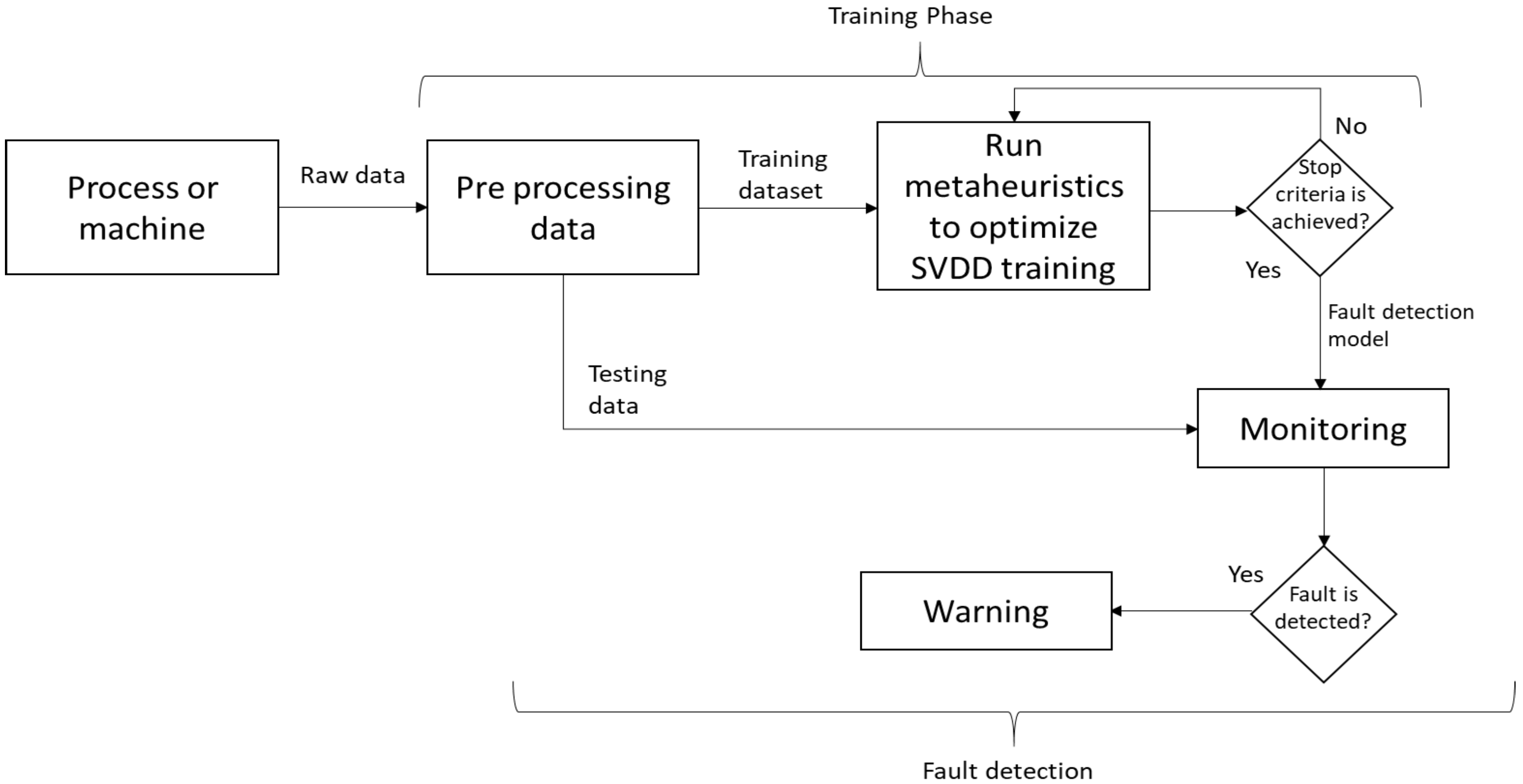
Figure 1. Fault detection system.
Applsci 10 09145 g001
Figure 2. F1 score box plot.
Applsci 10 09145 g002
Figure 3. Computational times box plot.
Applsci 10 09145 g003
Figure 4. F1 score Tukey test.
Applsci 10 09145 g004
Figure 5. Computational times Tukey test.
Applsci 10 09145 g005
Table 1. Variables description.
Description
x f 1 [ F ], Nozzle 1
x f 2 [ F ], Nozzle 2
x f 3 [Percent], Heating power zone 1
x f 4 [Percent], Heating power zone 2
x f 5 [Percent], Heating power zone 3
x f 6 [Percent], Heating power zone 4
x f 7 [Percent], Heating power zone 5
x f 8 [Percent], Heating power zone 6
x f 9 [in], Mold position value
x f 10 [in], Opening run
x f 11 [US ton], Closing force peak value
x f 12 [US ton], Closing force real value
x f 13 [s], Mold protection time
x f 14 [ F ], Oil temperature
x f 15 [ F ], Traverse
x f 16 [s], Cooling time
x f 17 [psi], Backpressure
x f 18 [ in 3 ], Volume end screw
holding pressure
x f 19 [psi], Holding pressure
x f 20 [ in 3 /s], Dosage power
x f 21 [psi], Pressure at Switchover
x f 22 [s], Cycle time
x f 23 [lbf-ft], Mean spin
x f 24 [lbf-ft], Peak value at spin
x f 25 [psi], Specific injection pressure
x f 26 [ in 3 ], Dosage volume
x f 27 [ in 3 ], Injection volume
x f 28 [s], Dosing time
x f 29 [s], Injection time
x f 30 [ F ], Cylinder zone 1
x f 31 [ F ], Cylinder zone 2
x f 32 [ F ], Cylinder zone 3
x f 33 [ F ], Cylinder zone 4
x f 34 [ft/s], Revolutions
x f 35 [Wh], Injection work
x f 36 [ in 3 ], Switching volume
Table 2. Parameters configuration for each algorithm.
SHOKHSSAPSO
Number of iterations200200200200
Population size50505050
v f = 0.02 , N f s = 3 w = 0.5
Other parameters D m a x = 0.005 , c 1 = c 2 = 2 ,
N m a x = 0.01
w n = 0.1 + 0.8 ( 1 i / 200 )
Table 3. F1 score—Times.
F1 ScoreTime
SHOKHSSAPSOSHOKHSSAPSO
10.96200.91890.96100.918976.6396112.7972139.2550207.6410
20.97440.91890.91890.918978.2157114.3666149.3458209.0972
30.95120.91890.97500.918977.4362113.8831129.8195208.6143
40.97440.91890.91890.918977.4033113.4381149.1254208.5458
50.97440.91890.91890.918977.6753114.3179147.2649207.9583
60.97500.91890.91890.918976.9510113.6539155.0708209.6714
70.97440.91890.97440.918977.3957114.0773142.7828211.6702
80.97500.91890.97500.933379.0279113.6960128.8649212.5049
90.97500.91890.91890.918978.7634113.6895143.1924208.9668
100.97440.91890.92110.918983.3741113.5960142.3234209.6382
110.96300.91890.97500.918980.4753113.8772116.8845210.7641
120.97500.91890.91890.918982.3348114.1014151.0041209.1223
130.97500.91890.91890.918979.5617114.0026149.3981208.3499
140.97500.91890.91890.918978.9463114.1080146.5968208.5490
150.97500.91890.91890.918979.7457113.7620151.1163210.4518
160.97440.91890.93510.918988.0263113.7218135.8897209.4198
170.95120.91890.91890.918978.0516113.8042147.1367209.8243
180.96200.91890.91890.918977.6847113.7368147.1347213.8261
190.97440.97440.91890.918977.964898.1384145.6228208.7176
200.96200.97440.91890.918979.1865114.2702152.3700208.1235
210.97440.97440.91890.918979.1609114.2038146.7939209.6390
220.97500.97440.91890.918976.4243114.1394148.8082210.0689
230.96300.97440.91890.918976.2201113.5049147.7095207.0849
240.97500.97440.91890.918978.9390113.6086145.8267208.5851
250.97500.97440.91890.918975.2608113.7726149.5031225.5017
260.97440.97440.97440.918974.3404113.8676129.5610210.0427
270.97440.97440.91890.918974.6434114.3396148.6370207.7600
280.96200.97440.97500.918974.9797113.4536131.1206209.6813
290.96200.97500.91890.918974.609993.0891154.4285207.8903
300.97500.97500.91890.918976.3885114.4280157.7352213.1721
Mean0.97020.94110.93210.919478.1942112.6482144.3441210.0294
Std0.00740.02770.02320.00262.81704.69049.17773.3325
Table 4. F1 score Kruskal–Wallis test.
SourceSSdfMSChi-sqp-Value
Columns56,089.6318,696.557.32.2188 × 10 12
Error60,398.9116520.7
Total116,488.5119
Table 5. Computational times Kruskal–Wallis test.
SourceSSdfMSChi-sqp-Value
Columns135,000345,000111.575.0394 × 10 24
Error899011677.5
Total143,990119
Publisher’s Note: MDPI stays neutral with regard to jurisdictional claims in published maps and institutional affiliations.