Abstract
The efficient data investigation for fast and accurate remaining useful life prediction of aircraft engines can be considered as a very important task for maintenance operations. In this context, the key issue is how an appropriate investigation can be conducted for the extraction of important information from data-driven sequences in high dimensional space in order to guarantee a reliable conclusion. In this paper, a new data-driven learning scheme based on an online sequential extreme learning machine algorithm is proposed for remaining useful life prediction. Firstly, a new feature mapping technique based on stacked autoencoders is proposed to enhance features representations through an accurate reconstruction. In addition, to attempt into addressing dynamic programming based on environmental feedback, a new dynamic forgetting function based on the temporal difference of recursive learning is introduced to enhance dynamic tracking ability of newly coming data. Moreover, a new updated selection strategy was developed in order to discard the unwanted data sequences and to ensure the convergence of the training model parameters to their appropriate values. The proposed approach is validated on the C-MAPSS dataset where experimental results confirm that it yields satisfactory accuracy and efficiency of the prediction model compared to other existing methods.
1. Introduction
Health state prediction in complex equipment or subsystems based on conventional methods such as physical modeling approaches became a very difficult task. Due to the need for deep knowledge of system components and their inner interactions, the modeling process complexity increased and became almost impossible. Even if the final model can be prepared under limited conditions, results might be misleading the prediction or not accurate enough due to poor generalization.
Nowadays, machine learning applications for Remaining Useful Life (RUL) estimation has received growing importance due to the availability of heterogeneous data, which in turn motivated researchers to boost the conventional RUL prediction paradigm with a variety of prediction approaches.
Continuous improvements of machine learning models make its use in Prognostic Health Management (PHM) more relevant [1]. It allows modeling systems behavior by only extracting important patterns from their retrieved data even without a prior knowledge of their internal characteristics. Unlike conventional paradigms, machine learning techniques aims to reduce modeling complexity with less human intervention and less computational costs.
For instance, Xiong Li et al. [2] used a Hidden Semi Markov Model (HSMM) to train SVM for RUL prediction. García et al. [3] designed a hybrid SVM-based swarm intelligence technique searching for the best training coefficients during RUL prediction of aircraft engines. Saidi et al. [4] combined Spectral Kurtosis (SK) to SVM to be able to construct an RUL predictor with a more meaningful feature mapping for wind turbine high-speed shaft bearings health prognosis. Zheng et al. [5] based on a hybrid model constructed a training formwork of the ELM model. They adopted a time window features scaling as a preprocessing and appropriate features selection step to guarantee an accurate prediction of RUL. Ordóñez et al. [6] proposed a hybrid autoregressive model combined with an improved SVM using genetic algorithm to build several estimation algorithms for early RUL prediction. Chen et al. [7] used a SVM-based similarity approach for RUL prediction with the same C-MAPPS dataset. It should be mentioned that all cited works could be classified as a hybrid model that aims to accurately predict the RUL by an unsupervised training or preprocessing of training data before a “single-batch” supervised training. However, time-varying data and parameter update is not considered in these cases, which is incompatible with data-driven prediction models able to address dynamic health deterioration of equipment according to internal or environmental conditions.
Neural networks with mini batch training are able to interact with flowing sequences of data and update the prediction model to satisfy changes in newly arrived ones. In [8], a new data-driven approach is introduced by Ben Ali et al. by training a Simplified Fuzzy Adaptive Resonance Theory Map (SFAM) neural network with Weibull Distribution (WD) to avoid time domain fluctuation during RUL prediction. Al-Dulaimi et al. [9] developed a mini batch hybrid deep NN that takes two paths for RUL estimation; the multidimensional feature extraction based on Long Short Term Memory (LSTM) and convolutional NN and the prediction path via a fusion algorithm. Wen et al. [10] constructed feature mapping and training schemes based on ensemble residual CNN and validated their training model with the K-fold cross-validation method after constructing several learners to predict RUL accurately. Xiang et al. [11] simplified the RUL prediction process of aircraft engines by the direct use of raw sensors measurements without a prior expertise in signal processing using a novel deep convolutional NN combined with a time window feature extractor. The prediction approaches used in these works are based on mini batch training interacting with data-driven sequences. Many training models were developed with different paradigms such as hybrid, ensemble, and deep learning attempting to access more meaningful data representations through an accurate prediction. However, the effect of dynamic changes at the level of the training mini batches of data on the training models is not discussed in this case, which may allow the weights and biases to diverge in some mini batches to under-fit gradually the NN. In other cases, the use of old mini batch training algorithms for NN such as the Backpropagation (BP) algorithm can increase computational costs and time consumption.
Through this analysis, the main challenges for RUL predictions task are:
- Update the training model based on data variation during time (adaptive learning).
- Decide whether the newly arrived data is important (new) for the training model or not.
- Make the training model in line with the actual health state of the equipment by giving more attention to newly acquired data and discarding gradually the old ones.
- Reduce time consumption during training.
In the recent decade, ELM has been widely used for prediction purposes due to the fast training and fewer parameters tuning based on the best fit of a linear function approximation [12]. Zhou et al. [13] proposed a Stacked ELM (S-ELM) where a stack of small ELMs is specially designed for solving large and complex data problems. Ben Ali et al. [14] presents a new unsupervised learning classification tool of extracted data based on the Adaptive Resonance Theory 2 (ART2) for high-speed shaft bearing prognosis. Li et al. [15] proposed an improved OS-ELM which is one of the ELM variants with an adaptive forgetting factor and an update selection strategy to predict gas utilization ratio using time-varying data. Yang et al. [16] developed a new approach of regularization of the recursive learning of the OS-ELM to reduce over-fitting and both empirical and structural risks of the prediction model. Lu et al. [17] enhanced the recursive learning of the OS-ELM by introducing ensemble Kalman filter propagation for output weights tuning of NN under RUL prediction of aircraft engines. Yin et al. [18] proposed a (TD-RLS(λ)) with a forgetting factor to enhance the RLS adaptation to linear function approximation by updating its parameters based on environmental feedback.
OS-ELM can address online learning in real time such as our RUL prediction problem without iterative tuning, which strongly contribute to computational costs reduction. Training rules of OS-ELM allows recursive learning with any driven chunks of data easily even with different or fixed sizes. In general, one of the limitations of OS-ELM or ELM algorithms is the interpolation caused by the pseudo inverse of the matrix [19], which makes ELM variants suffering from structural risks.
In this paper, an improved data-driven approach based on OS-ELM is proposed for RUL estimation to enhance the novelty of the prediction algorithm and its adaptability to time-varying data. In fact, the main contributions of this work attempting to solve adaptive learning and ill-posed problems are:
- SAEs based OS-ELM is modified for best features extraction and selection via unsupervised learning.
- An OS-ELM is introduced.
Tikhonov regularization is involved to reduce structural risk and over-fitting by minimizing the norm of the training weights.
Dynamic forgetting of old data, USS and TD error objective functions are all integrated into both SAEs and OS-ELM to achieve better accuracy and adaptability to newly arrived data.
The proposed approach is applied to the public dataset of the turbofan engine [20], where obtained results compared to other recent used approaches in the literature show higher performance.
The remainder of this work is organized as follows: In Section 2, a general description of the turbofan engine dataset is presented. Section 3 elaborates on the proposed approach used in this paper. Section 4 illustrates and discusses the experimental results where the performances of the proposed learning scheme are showcased and compared to other data-driven methods. Finally, Section 5 concludes with a summary.
2. Dataset Description
The C-MAPSS dataset consists of four different subsets, where each dataset consists of multiple multivariate time series and describes different operating conditions and faults modes for different engines. Each dataset is divided into training and testing sets.
In our work, we have used the subset FD001 and only a single operating condition and one fault mode are considered. At the beginning of each time series, the engine is considered as normally functioning according to initial conditions and at a certain level, it starts deteriorating gradually by losing its performances until the failure.
Each dataset contains 26 columns which are considered as the input features of the prediction model, each column contains information about engine number, time cycles, sensors measurements, and operational conditions of the operating engine [21].
The dataset describes life cycles of 100 different engines with a big amount of training samples where their characteristics changes in time. The reason behind studying this type of data is to address dynamic programming and adaptive learning to solve higher dimensional space problems.
Figure 1 illustrates an example of sensors measurement variation and its corresponding RUL degradation function of the first engine from the chosen dataset, where the different colors represent different sensors.
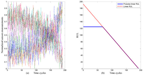
Figure 1.
(a) Normalized sensors measurement. (b) Corresponding RUL to sensors measurement.
3. The Proposed Approach
Figure 2 indicates the methodology adopted for RUL prediction in this work. Essentially there are two distinctive parts: Dataset preparation and prediction model training.
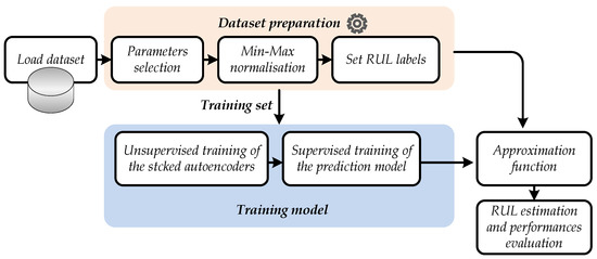
Figure 2.
Flowchart of the proposed RUL prediction approach.
3.1. Dataset Preparing
The preparation of the dataset is firstly initialized with an appropriate feature selection where only the most significant and sensitive features will be chosen. Each one must describe a certain attitude of degradation level or gradual time-varying behavior in each time cycle. Measurements that do not represent any variation during operating cycles will not contribute to the learning process. In fact, their noncorrelation with the desired RUL can disturb the training model and makes it more sensitive to over-fitting and other ill-posed problems. In our experiments, we chose only 10 parameters for RUL prediction whose indices are: {7, 8, 9, 12, 14, 16, 17, 20, 25, 26}. After that these features are scaled in the interval [0–1] using a min-max normalization procedure before training or testing. Finally, each time series will be labeled according to the piecewise linear RUL function as proposed in [1,22] and shown previously in Figure 1.
3.2. Prediction Model Training
The training of the RUL prediction model passes by two different steps: Training of the SAEs and OS-ELM. In this paper, both unsupervised and supervised learning are performed based on the proposed algorithm. Therefore, before going any further, first, we will explain the fundamentals of basic OS-ELM. Then, the proposed OS-ELM will be explained in detail for both unsupervised and supervised learning strategies.
3.2.1. Basic OS-ELM
Since ELM learns a big amount of data at once, the output weights β of the hidden layer are also tuned for once and cannot be updated. Therefore, a new problem of weights updating appears when data change with time. Consequently, ELM releases the OS-ELM as one of its variants that depend on an online learning attitude with chunks in varied or fixed size, as it also could learn data that come consecutively in one by one instance [23].
OS-ELM experimentally has given the training rules as explained in the following steps:
For a given small dataset , initialization of the network parameters:
- Generate randomly all the input weights and hidden layer biases . The parameters of hidden nodes (weights and biases) must be normalized between {-1,1} [24].
- Calculate the initial hidden layer output Hk (k = 0) as the same basic ELM theories as presented in Equation (1), where G can be generated independently from the training data according to any continuous bounded piecewise activation function.
- Calculate the first output weight matrix βk (k = 0) as shown in Equation (2).
- Set k = 0.
- Recursive updating of β for new coming mini batches.
- Calculate the new hidden layer Hk+1; Equation (1).
- Update the output weight matrix βk+1; Equation (4).
- Then, set k = k + 1.
3.2.2. Proposed OS-ELM
In the proposed algorithm we have added a regularization parameter C to reduce empirical and structural risks [16] during the initialization phase. Therefore, Equation (3) will be changed into Equation (8) given below [25], where .
After the training model is initialized, the USS-based TD objective function is proposed to adopt the RLS weights to the new data variations [18]. Furthermore, we proposed, based on [8,18,26], a new DFF formula that is proposed as illustrated in Equation (10), so Equations (4) and (5) will be changed, respectively, into (9) and (10).
The dynamic forgetting factor changes according to the proposed formula in Equation (13) where and .
3.2.3. Training of the Proposed Network
SAEs are serially trained autoencoders. The encoded features of an autoencoder are considered as the inputs of the next one as shown in Figure 3.
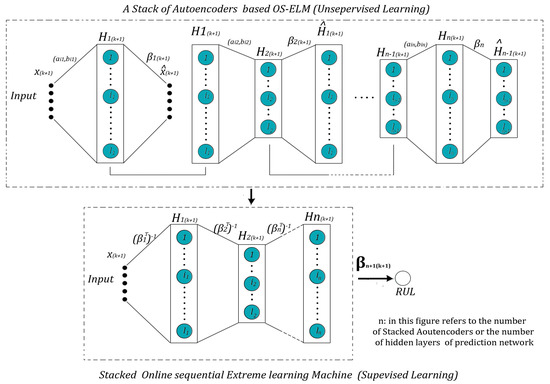
Figure 3.
Proposed NN (Neural Networks) for RUL prediction.
Both of the unsupervised and supervised training in our proposed approach carried with fixed sizes of mini batches to verify the objective function of TD error in Equation (10) and to avoid a mismatch dimensions error for programming reasons. The results of the mapping of the SAEs are directly used for fine-tuning the RUL prediction network, the update of supervised and unsupervised training models is simultaneously achieved.
During the training of the SAEs, we have to change the targets in the above-proposed equations to be the same as the input [13]. Therefore, Equations (1), (2), and (10) must be changed to fit the training process of the SAEs.
Our main contribution to modify the autoencoder in this work is that the basic ELM theories for training the autoencoder show that: “After training the Autoencoder, we can encode features using the transpose of output weights matrix [13], Equation (14)”. However, mathematically it is proven that the best encoding can be obtained by using the inverse matrix of the transpose of output weights as shown in Equation (15). The proposed formula is tested experimentally and proved its accuracy [27].
An important note that we should take into consideration during the training of the SAEs is that after the initialization phase, we are no longer in need of the randomly generated input weights and we will use the formula in Equation (16) instead of the one in Equation (1).
where Xk+1 are the kth+1 mini batch of inputs of the training set.
4. Experiments, Results, and Discussion
The training parameters of the proposed algorithm are tuned after repeating the experiment in reason to attempt the best score value in Equation (17) and the minimum RMSE using Equation (18) for the test set in both Equations (17) and (18).
According to the PHM 2008 challenge [22], the scoring function penalizes the latent prediction more than early ones for maintenance reasons. Too late prediction might delay maintenance operations, and too early prediction might not be harmful but consumes more maintenance resources. Figure 4 explains that the sparseness of the RMSE and score function towards higher values is less than the others towards zero, which confirms the credibility of the results.
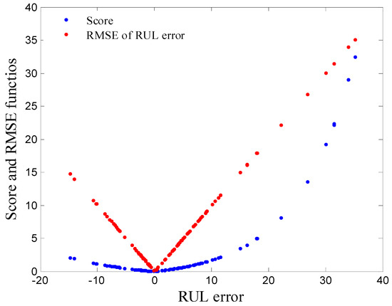
Figure 4.
Scoring functions for the testing set results.
Experimental results lead to the parameters shown in Table 1.

Table 1.
Training parameters of the proposed algorithm.
A set of training mini batches was ignored during training of the RUL prediction models with the contribution of the USS strategy. This can contribute to training time reduction and avoiding divergence of training weights.
Figure 5 illustrates the reaction of USS strategy towards the useless mini batches by showing the indexes of ignored and selected mini batches. It is obvious that USS conditions shown previously in Equation (9) are confirmed in Figure 5. The RMSE error of each selected chunk of data is bigger than the one before it.
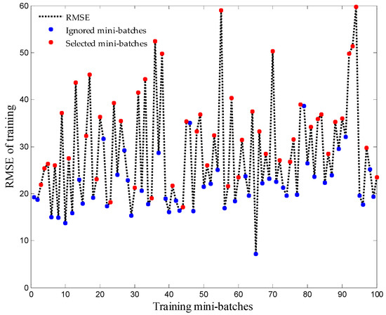
Figure 5.
The behavior of USS (Updated Selection Strategy) strategy towards the unused training mini batches.
During training, the DFF by the intervention of TD error minimization function-based RLS can contribute to the prediction algorithm adaptation towards variations in the newly arrived data. By adapting weights gradually to enhance the approximation function, the accuracy of the prediction will remain stable and always converges to the desired value. Figure 6 shows the variation of DFF during training. If the TD changes too much, it means that the new coming training data has also different characteristics from the first ones, which consequently forces the training weights β to adapt towards these new changes. The adaptation of β is a result of updating the forgetting factor λ, and the amount of changes is controlled by the user hyper-parameters expressed in Table 1.
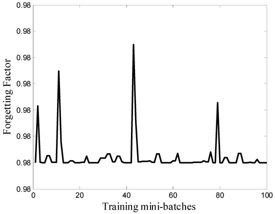
Figure 6.
Dynamic forgetting function behavior during training.
The training model was tested using new data (unknown to the model) from a test set of FD001. Additionally, the example of curve fitting of the RUL target function in Figure 7 proves that the proposed approach has an acceptable performance. The response of the designed network in Figure 7 is plotted using a set of different life cycles of different engines from the test set.
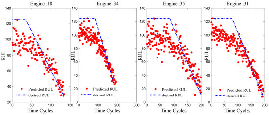
Figure 7.
RUL prediction function compared to desired function.
The proposed approach performances are compared with a set of other recent approaches in the literature. The results from Table 2 indicate that the proposed algorithm has the ability to achieve a low score value depending on less training samples and less training time.
Table 2.
Performance results compared to other recent RUL prediction approaches.
5. Conclusions
A new online sequential training scheme is presented in this work for the RUL prediction of aircrafts engines. The proposed training model explained that by accepting any training mini batch of time-varying data in every update without taking into consideration the divergence of the weights at a certain level, the training model will no longer behave positively to attain the needed approximation and generalization for newly arrived data.
So far, the proposed USS strategy is involved in over-fitting reduction and accurate feature selection. The DFF-based TD error estimation plays a key role in weights adaptation between the current and the next training mini batches. The accurate features mapping based on robust unsupervised learning can solve the higher dimensional data problems. The experimental results prove that the new learning scheme for higher dimensional dynamic data is fast and accurate making it a competitive candidate for time-varying data prediction problems.
In the literature, C-MAPPS dataset is studied and investigated with different machine learning models. One of the important issues that has not yet been discussed is that sensors measurements are contaminated with noise of unknown sources and behavior. Therefore, future investigations will be focused on enhancing the proposed approach accuracy considering noisy measurements.
Author Contributions
Conceptualization, T.B. and L.-H.M.; Methodology, T.B. and L.-H.M.; Software, T.B.; Validation, T.B., L.-H.M., O.K., L.S., and M.B.; Formal Analysis, T.B., L.-H.M., O.K., L.S., and M.B.; Investigation, T.B.; Writing—Original Draft Preparation, T.B.; Writing—Review & Editing, T.B., L.-H.M., O.K., L.S., and M.B.; Supervision, L.-H.M. All authors have read and agreed to the published version of the manuscript.
Funding
This research received no external funding.
Conflicts of Interest
The authors declare no conflict of interest.
Abbreviations
| C-MAPSS | Commercial Modular Aero Propulsion System Simulation |
| DFF | Dynamic Forgetting Factor |
| ELM | Extreme Learning Machine |
| NN | Neural Networks |
| OS-ELM | Online Sequential ELM |
| RLS | Recursive Least Squares |
| RMSE | Root Mean Squared Error |
| RUL | Remaining Useful Life |
| SAEs | Stacked Autoencoders |
| SVM | Support Vector Machine |
| TD | Temporal Difference |
| USS | Updated Selection Strategy |
| A | Input weight matrix |
| BI | Vector of biases |
| C | Regularization parameter |
| d | Prediction difference |
| e | Prediction error (matrix) |
| G | Activation function |
| H | Hidden layer |
| k | Index of recursive learning |
| K | Gain matrix of RLS |
| l | Hidden nodes number |
| n | Size of mini batch |
| N | Size of training data |
| S | Score function |
| T | Target samples |
| Z | Testing samples number |
| (T) | Transpose matrix |
| β | Output weights |
| λ | Forgetting factor |
| γ | Discounting factor of TD error |
| δ | Temporal difference |
| μ | Sensitivity factor |
| (−1) | Pseudo inverse of the matrix |
References
- Babu, G.S. Deep Convolutional Neural Network Based Regression Approach for Estimation of Remaining Useful Life. Lect. Notes Comput. Sci. 2016, 9642, 214–228. [Google Scholar]
- Xiong, X.; Li, Q.; Cheng, N. Remaining useful life prognostics of aircraft engine based on fusion algorithm. In Proceedings of the 2016 IEEE Chinese Guidance, Navigation and Control Conference (CGNCC), Nanjing, China, 12–14 August 2017; pp. 628–633. [Google Scholar]
- Nieto, P.J.G.; García-Gonzalo, E.; Lasheras, F.S.; Juez, F.J.D. Hybrid PSO-SVM-based method for forecasting of the remaining useful life for aircraft engines and evaluation of its reliability. Reliab. Eng. Syst. Saf. 2015, 138, 219–231. [Google Scholar] [CrossRef]
- Saidi, L.; Ali, J.B.; Bechhoefer, E.; Benbouzid, M. Wind turbine high-speed shaft bearings health prognosis through a spectral Kurtosis-derived indices and SVR. Appl. Acoust. 2017, 120, 1–8. [Google Scholar] [CrossRef]
- Zheng, C.; Liu, W.; Chen, B.; Gao, D.; Cheng, Y.; Yang, Y.; Peng, J. A Data-driven Approach for Remaining Useful Life Prediction of Aircraft Engines. In Proceedings of the 2018 21st International Conference on Intelligent Transportation Systems (ITSC), Maui, HI, USA, 4–7 November 2018; pp. 184–189. [Google Scholar]
- Ordóñez, C.; Lasheras, F.S.; Roca-Pardiñas, J.; Juez, F.J.d. A hybrid ARIMA–SVM model for the study of the remaining useful life of aircraft engines. J. Comput. Appl. Math. 2019, 346, 184–191. [Google Scholar] [CrossRef]
- Chen, Z.; Cao, S.; Mao, Z. Remaining useful life estimation of aircraft engines using a modified similarity and supporting vector machine (SVM) approach. Energies 2018, 11, 28. [Google Scholar] [CrossRef]
- Ali, J.B.; Chebel-Morello, B.; Saidi, L.; Malinowski, S. Accurate bearing remaining useful life prediction based on Weibull distribution and artificial neural network. Mech. Syst. Signal Process. 2014, 1–23. [Google Scholar]
- Al-Dulaimi, A.; Zabihi, S.; Asif, A.; Mohammadi, A. A multimodal and hybrid deep neural network model for Remaining Useful Life estimation. Comput. Ind. 2019, 108, 186–196. [Google Scholar] [CrossRef]
- Wen, L.; Dong, Y.; Gao, L. A new ensemble residual convolutional neural network for remaining useful life estimation. Math. Biosci. Eng. 2019, 16, 862–880. [Google Scholar] [CrossRef] [PubMed]
- Li, X.; Ding, Q.; Sun, J.Q. Remaining useful life estimation in prognostics using deep convolution neural networks. Reliab. Eng. Syst. Saf. 2018, 172, 1–11. [Google Scholar] [CrossRef]
- Huang, G.B. An Insight into Extreme Learning Machines: Random Neurons, Random Features and Kernels. Cognit. Comput. 2014, 6, 376–390. [Google Scholar] [CrossRef]
- Zhou, H.; Huang, G.-B.; Lin, Z.; Wang, H.; Soh, Y.C. Stacked Extreme Learning Machines. IEEE Trans. Cybern. 2014, 99, 1. [Google Scholar]
- Ben, J.; Harrath, S.; Bechhoefer, E.; Benbouzid, M. Online automatic diagnosis of wind turbine bearings progressive degradations under real experimental conditions based on unsupervised machine learning Online automatic diagnosis of wind turbine bearings progressive degradations under real experimental con. Appl. Acoust. 2018, 132, 167–181. [Google Scholar] [CrossRef]
- Li, Y.; Zhang, S.; Yin, Y.; Xiao, W.; Zhang, J. A novel online sequential extreme learning machine for gas utilization ratio prediction in blast furnaces. Sensors 2017, 17, 8. [Google Scholar] [CrossRef] [PubMed]
- Yang, L.; Yang, S.; Li, S.; Liu, Z.; Jiao, L. Incremental laplacian regularization extreme learning machine for online learning. Appl. Soft Comput. J. 2017, 59, 546–555. [Google Scholar] [CrossRef]
- Lu, F.; Wu, J.; Huang, J.; Qiu, X. Aircraft engine degradation prognostics based on logistic regression and novel OS-ELM algorithm. Aerosp. Sci. Technol. 2019, 84, 661–671. [Google Scholar] [CrossRef]
- Yin, B.; Dridi, M.; El Moudni, A. Recursive least-squares temporal difference learning for adaptive traffic signal control at intersection. Neural Comput. Appl. 2019, 31, 1013–1028. [Google Scholar] [CrossRef]
- Huang, G.; Member, S.; Zhou, H.; Ding, X.; Zhang, R. Extreme Learning Machine for Regression and Multiclass Classification. IEEE Trans. Syst. Man Cybern. Part B 2012, 42, 513–529. [Google Scholar] [CrossRef] [PubMed]
- Saxena, A.; Saad, A. Evolving an artificial neural network classifier for condition monitoring of rotating mechanical systems. Appl. Soft Comput. J. 2007, 7, 441–454. [Google Scholar] [CrossRef]
- Saxena, A.; Goebel, K.; Simon, D.; Eklund, N. Damage propagation modeling for aircraft engine run-to-failure simulation. In Proceedings of the 2008 IEEE ICPHM, Denver, CO, USA, 12–15 October 2008; pp. 1–9. [Google Scholar]
- Heimes, F.O. Recurrent neural networks for remaining useful life estimation. In Proceedings of the 2008 IEEE ICPHM, Denver, CO, USA, 12–15 October 2008; pp. 1–6. [Google Scholar]
- Huang, G.B.; Liang, N.Y.; Rong, H.N.; Saratchandran, P.; Sundararajan, N. On-line sequential extreme learning machine. In Proceedings of the 2005 IASTED ICCI, Calgary, AB, Canada, 4–6 July 2005; pp. 1–6. [Google Scholar]
- Lan, Y.; Soh, Y.C.; Huang, G.B. A Constructive Enhancement for Online Sequential Extreme Learning Machine. In Proceedings of the 2009 International Joint Conference on Neural Networks, Atlanta, GA, USA, 14–19 June 2009; pp. 1708–1713. [Google Scholar]
- Gu, Y.; Liu, J.; Chen, Y.; Jiang, X. Constraint Online Sequential Extreme Learning Machine for lifelong indoor localization system. In Proceedings of the 2014 International Joint Conference on Neural Networks, Beijing, China, 6–11 July 2014; pp. 732–738. [Google Scholar]
- Kiakojoori, S.; Khorasani, K. Dynamic neural networks for gas turbine engine degradation prediction, health monitoring and prognosis. Neural Comput. Appl. 2016, 27, 2157–2192. [Google Scholar] [CrossRef]
- Berghout, T. Autoencoders. 2019. Available online: https://www.mathworks.com/matlabcentral/fileexchange/66080-autoencoders (accessed on 21 October 2019).


© 2020 by the authors. Licensee MDPI, Basel, Switzerland. This article is an open access article distributed under the terms and conditions of the Creative Commons Attribution (CC BY) license (http://creativecommons.org/licenses/by/4.0/).