Abstract
Planing boat dynamics are a complex phenomenon and the maneuver forces acting on these kind of hulls are difficult to predict. In the current work, a mathematical model of a two-dimensional impact with three degrees of freedom (3DOF) is developed. The model was used to study wedge sections with knuckles, the vertical, horizontal, and rotational motion are considered. Pressure distribution, forces, and motion during the impact, considering both free fall and forced motion, are evaluated. The commercial CFD (Computational flow dynamics) software Star-CCM+ V9.06 was used to validate the formulation. Simulations with one, two, and three degrees of freedom were carried out, and the results were compared with CFD simulations, experimental data, and numerical solutions by others authors. The results show a good agreement with the authors. The model is extended to three dimensions applying slender body theory, and the forces in the hull are computed. The formulation allows evaluating the seakeeping with cross flow, dynamic stability, and manoeuvrability of planing boats with variable sections over the length.
1. Introduction
Planing boats are used in sports, tourism, and missions, such as patrol, rescue, and interdiction in rivers and seas. These boats can reach velocities near to 50 kn, and due to operational conditions, impact loads appear due to the waves, and vertical accelerations greater than 20 g can be attained [1]. Furthermore, there is instability of the boat, and the working conditions produce negative effects for the crew members, such as fractures in the legs and arms, and spinal injuries. Wagner [2] developed a mathematical model based on potential flow; the model evaluates the pressure distribution on the symmetric impact without flow separation. Toyama [3] extended the model developed by Wagner [2] for sections with asymmetrical entry and vertical velocity without flow separation.
Vorus [4] used potential flow and boundary elements theory to study the symmetrical impact with flow separation. Xu et al. [5] extended the model developed by Vorus [4] for sections with asymmetrical entry and vertical velocity with flow separation. Judge and Troesch [6] extended the model developed by Xu et al. [5] and the critical condition that causes the flow separation from the keel was found. Xu et al. [7] followed a procedure similar to Vorus [4], using potential flow and boundary elements theory to study the impact of asymmetric sections with vertical and horizontal velocity without flow separation. Semenov and Iafrati [8] simulated the asymmetry impact with horizontal velocity using the mapping method and complex potential flow; furthermore, a criteria to predict the critical condition for flow separation from the keel was developed.
Xu et al. [9], used boundary elements to model the impact of sections with three degrees of freedom and free fall without flow separation. Wei et al. [10] modelled the impact of asymmetric sections and three degrees of freedom and free fall with flow separation through potential flow theory and the surface interpolation method (Constrained Interpolation Profile, CIP). Bao et al. [11] modelled the free fall impact with three degrees of freedom using the boundary element method and potential flow. The dynamic responses of wedge sections were evaluated during the impact.
Seif et al. [12] simulated the two-dimensional impact of asymmetric sections with vertical velocity through CFD tools. Bilandi et al. [13] simulated the asymmetric impact with CFD tools using the finite volume method and volume of fluid, the pressure distribution and the free surface during the impact were evaluated. The results show a good agreement with Toyama [3] and Semenov and Iafrati [8]. Tascón et al. [14] simulated the impact of asymmetric sections with vertical and horizontal velocity, in order to evaluate the forces over the boat using the slender body theory.
Algarín [15] simulated the asymmetric impact for vertical and horizontal velocity with CFD. The 2D+t theory was used to evaluate the forces in a boat sailing under asymmetric and steady conditions. The critical conditions that caused the flow separation from the keel were found with CFD tools. Algarín and Tascón [16] extended the model developed by Wagner [2] for asymmetric sections with vertical velocity and flow separation. Bilandi et al. [17] applied the 2D+t theory to evaluate the resistance and dynamic trim in single-stepped hulls, and the results showed reasonably good agreement with experimental data for a Froude number up to 2.0. Tascón and Algarín [18] simulated the impact of asymmetric sections with vertical and rotational velocity. The 2D+t theory was used to model the forced oscillation test during roll for planing boats.
Tavakoli et al. [19] used the 2D+t theory to evaluate planing boats sailing with asymmetry and steady conditions. In virtual tests, the drift angle was varied and the equilibrium angles of trim and heel were found for different velocities. The results of equilibrium angles and resistance were close to the experimental data obtained in towing tank tests. The study of the flow separation from the knuckles allows for evaluation of the dynamic pressures in the wetted chine region in planing hulls. This region is import to analyse of the dynamics and dynamics stability of the planing boats.
Figure 1 shows the impact of a wedge section with a symmetry entry, where is the deadrise angle, is the half wetted beam, is the wedge immersion, b is the section beam, d is the vertical distance between keel and knuckle, and and are the horizontal and vertical axes. The energy equation for a potential flow is:
where is the potential function of the fluid, is the pressure, and is the density of the liquid. The potential function equation for the symmetry impact proposed by Wagner [2] is:
where is the variation with the time for the half wetted beam, for a wedge section this parameter is evaluated as:
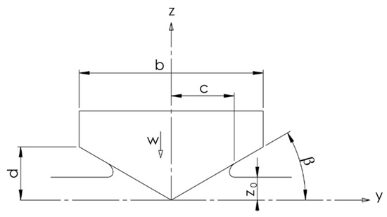
Figure 1.
Impact with symmetry entry.
Figure 2 shows the asymmetrical impact of a wedge section, Toyama [3] extended the model developed by Wagner [2] for the impact with asymmetrical entry and introduced the asymmetry parameter μ, ϕ is the heel angle, is the wetted half beam in the right side, is the wetted half beam in the left side, and are defined as:
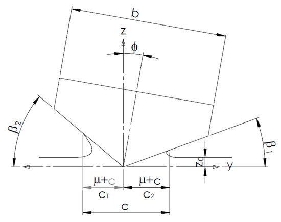
Figure 2.
Impact with asymmetry entry.
The equation for potential flow form Toyama [3] is:
The pressure in the asymmetry impact is computed as:
The parameters of the model are evaluated as:
where
The aim of this paper is to develop a mathematical model of a two-dimensional impact with three degrees of freedom (3DOF) and apply the results to study planing hulls. In the current work, the model by Toyama [3] is extended to the asymmetric impact with vertical velocity , horizontal velocity , and rotational velocity . Furthermore, the flow separation from the knuckles is considered. A formulation to extend the results to three dimensions is proposed, the model can be used to study the dynamics of planing hulls with six degrees of freedom. The six motions cannot be evaluated with the traditional seakeeping models by Zarnick [20], Garmé [21], and Olausson and Garmé [22].
2. Mathematical Formulation
Figure 3 shows the parameters of the impact with three degrees of freedom, due to the relative motion of the wedge with the water. The new components appearing for vertical and tangential velocity are calculated as:
where , , , and are the vertical velocity and tangential velocity in the right and left side of the wedge respectively, is the relative velocity in a point due to the rotation, and is the angle between the vector and the tangential vector to the section, as shown in Figure 4. The parameters are calculated as:
where and are the horizontal distance and vertical distance in a point on the hull to the CG (Gravity centre), is the total distance between the centre of rotation and a point in the wedge, and is the angle between the vector to the horizontal axis .
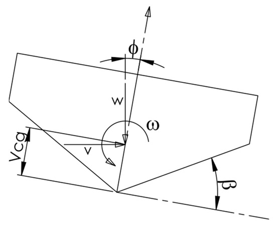
Figure 3.
Impact with three degrees of freedom.
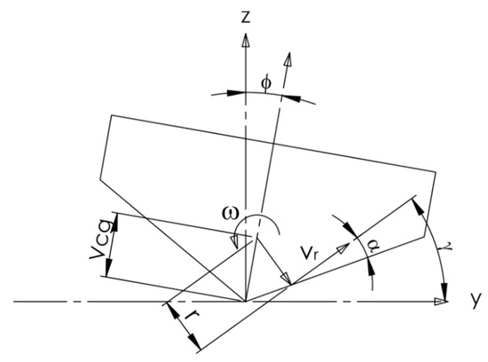
Figure 4.
Asymmetric impact with rotational motion.
The potential function that represents the flow during the impact with three degrees of freedom is:
The models by Wagner [2] and Toyama [3] over-predict the pressure, and two correction factors are proposed: a correction factor of the deadrise angle , and a correction factor for the jet energy , is a correction factor that depends on the deadrise angle of the wedge. By substitution in Equation (1) the pressure distribution can be computed as:
where is a correction factor due to jet energy, which is evaluated as:
In the two dry chines-phase, the values , , , and are calculated with Equations (14)–(17). In the one wet chines-phase, the boundary condition is:
where is the horizontal distance between the keel and knuckle in the right side, the one wet chine-phase starts when . In Equation (33), the effect of the acceleration is not considered. The half beam in the left side is evaluated according with Toyama [3]:
Solving Equations (33)–(36) the values for , ,, and are calculated for the flow separation in the right side. When the two dry chines-phase occurs the boundary conditions are the set presented in Equation (37). The equations are solved in a coupled form to find the values of , , , and .
where is the horizontal distance between the keel and knuckle in the left side, the two wet chine-phase starts when . The sectional forces can be computed as:
where is the vertical force, is the horizontal force, is the roll moment in the keel, is the roll moment in the CG of the section, and and are the horizontal wetted coordinate in the right side and left side respectively. In case of prescribed motions, these equations can be used to evaluate the pressure and forces in the section. The vertical force can be computed as:
where
where and are evaluated as:
The horizontal force can be evaluated as:
where
The roll moment of the section in the CG is calculated as:
where
The coefficients , , , , , , , , , , , and are computed as:
Figure 5 shows the forces diagram in the section, the balance of force can be written as:
where is the mass of the wedge, is the gravity, and is the inertia of the section. Furthermore:
where , , and are the vertical force, horizontal force, and roll moment due to hydrostatic pressure, coupling the equations:
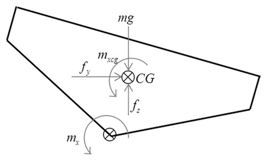
Figure 5.
Forces diagram in the wedge.
In case of two degrees of freedom, rotation, and vertical motion, the equations of motion are:
Solving Equations (82) and (83), the free fall impact for wedge sections with two and three degrees of freedom can be studied.
3. CFD Modelling
The CFD software Star-CCM+ V9.06 is used in order to simulate the two-dimensional impact of wedge sections on water. The volume of fluid (VOF) approach was used to simulate the water-air mix. Water and air were modelled as incompressible, inviscid fluids, and unsteady, while the wedge motion was modelled as a rigid body motion. Finally, the wedge motion was modelled with two approaches. In case of impact with prescribed motion, a rigid body with the rigid mesh approach was used. In the case of free fall impact, the motions were modelled with mesh morphing. The effect of gravity was taken into consideration. The VOF formulation used in the CFD includes the HRIC (High-Resolution Interface Capturing) method, the controls of this method are the lower currant number Cul that was set at 0.5, the upper currant number Cuu that was set at 1.0, and the angle factor Cθ that was set at 0.05. Figure 6 shows the computational domain at 10 b wide and 4.7 b high, and the boundary conditions as: wall in the base, verticals walls, wedge boundaries, and a pressure outlet in the top boundary.
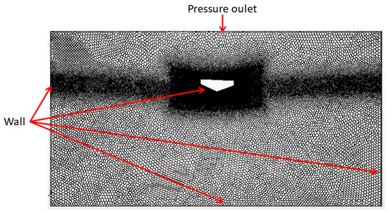
Figure 6.
Computational domain.
The mesh was developed with polyhedral elements and a mesh refinement was performed in the free surface area around the wedge and wedge walls. Figure 6 shows the mesh for the computational domain after the mesh independence analysis was carried out for a free fall test with 3DOF.
The converge analysis was carried out according to ITTC (International Towing Tank Conference) [23], the global convergence ratio Rg, the global accuracy order pg, the global correction factor Cg, and the global uncertainty Ug were computed using the norm L2. We considered 425 points of the solution, the accuracy order was calculated according to Roache [24], and the base size of the mesh and time step were changed. Figure 7a shows the time series for angular acceleration () when the impact with three degrees of freedom is considered. Four different mesh sizes were evaluated, and we noticed that the results for mesh sizes 4.3 × 10⁵ and 6.0 × 10⁵ cells are superposed. Figure 7b shows the time series for angular acceleration when three different time steps are considered. For time steps Δt = 1 × 10⁻⁴ s and 2 × 10⁻⁴ s the curves are superposed, and a time step of 2 × 10⁻⁴ s was selected. Table 1 shows the base size of the mesh, the number of elements, and the parameters of the study, 0 < Rg < 1. The solution is monotonic convergent, the accuracy order is 0.647, the global uncertainty is 28.1% of the maximum acceleration, the convergence ratios in the crest and hollow were computed, and they are convergent.
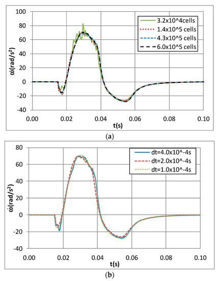
Figure 7.
Mesh independence analysis. (a) Angular acceleration vs. time, and size independence. (b) Angular acceleration vs. time, and time independence.

Table 1.
Mesh independence analysis.
Figure 8 shows the free surface during the impact in free fall of a wedge with two degrees of freedom. When the wedge touched the water is considered to be t = 0. At the beginning of the impact the flow is parallel to the section (Figure 8a–c), the flow separates from the both sides of the section after the jet reaches the chine (Figure 8d–f).
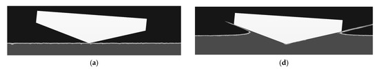
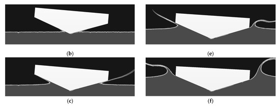
Figure 8.
Free surface during the free fall impact of a wedge with two degrees of freedom. (a) t = 0.0000 s. (b) t = 0.0044 s. (c) t = 0.0174 s. (d) t = 0.0234 s. (e) t = 0.0374 s. (f) t = 0.0654 s.
4. Results and Analysis
In order to validate the mathematical model, simulation results were compared to CFD computation, experiments, and results carried out by other authors. The following parameters are defined:
where is the pressure coefficient, is the horizontal force coefficient, is the vertical force coefficient, is the roll moment coefficient, and is the non-dimensional time.
4.1. Impact with One Degree of Freedom
The equation system is solved forcing , , and , in order to study the impact with one degree of freedom. Figure 9 shows the results for pressure distribution during the impact for a wedge section with symmetry entry and β = 20°. The results of the mathematical model are compared with Wagner [2] and CFD simulations. They show good agreement with CFD simulations, the error in the pressure peak respect to [15] is 2.99%, the correction factors suggested reduce the over prediction of the model by Wagner [2]. Figure 10 shows the force during the immersion of a wedge with β = 20°. The results attained from the mathematical model were compared with Tveitnes [25], it is noticed that the forces before and after the flow separation from the knuckle show a good agreement, the error in the vertical peak force is 2.04% respect to Tvenies [25] and 8.12% respect to [15].
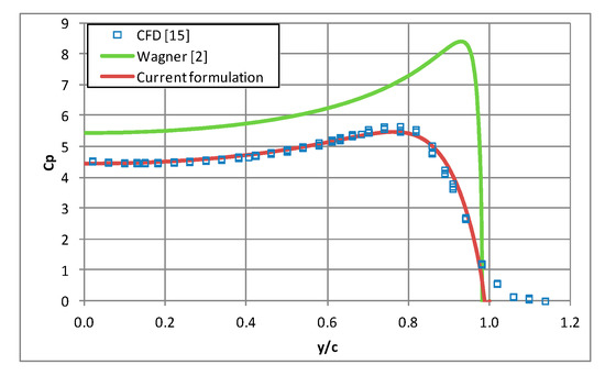
Figure 9.
Cp vs. y, β = 30°, impact with symmetry entry.
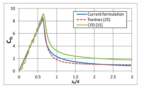
Figure 10.
Cfz vs. z0/d, β = 20°, impact with symmetry entry.
4.2. Impact with Two Degrees of Freedom
The equations system is solved forcing , in order to analyse the impact with two degrees of freedom, vertical motion, and horizontal motion. Figure 11 shows the pressure distribution before the flow separation from the knuckle for a wedge with β1 = 20°, β2 = 30°, and velocity ratio v/w = 0.5. The results are compared with CFD simulation performed by Algarín [15], presenting a good agreement, the error in the peak pressure is 7.27%, with respect to [15].
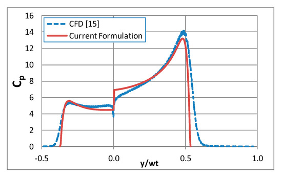
Figure 11.
The pressure distribution during impact with horizontal velocity β1 = 20°, β2 = 30°, and v/w = −0.50.
Figure 12 shows the results of vertical force for a wedge with β1 = 20°, β2 = 30°, and velocity ratio v/w = −1.0. The results before and after the flow separation from the knuckle are compared with the CFD results obtained by Algarín [15], presenting reasonably good agreement.
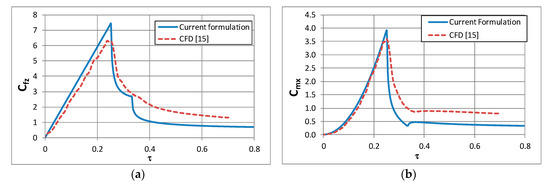
Figure 12.
Forces variation during impact with horizontal velocity, β1 = 20°, β2 = 30°, and v/w = −1.0. (a) Vertical force during the impact. (b) Roll moment during the impact.
The equations system is solved forcing in order to analyse the impact with two degrees of freedom, vertical motion, and rotation motion. Figure 13 shows the pressure distribution before the flow separation from the knuckle for a wedge with β = 45°, Vcg = 0.25 m, ω = −2.5 rad/s, w = 5 m/s, and initial heel angle ϕ0 = −10. The results are compared with Xu G. [9] and the CFD simulation, presenting good agreement.
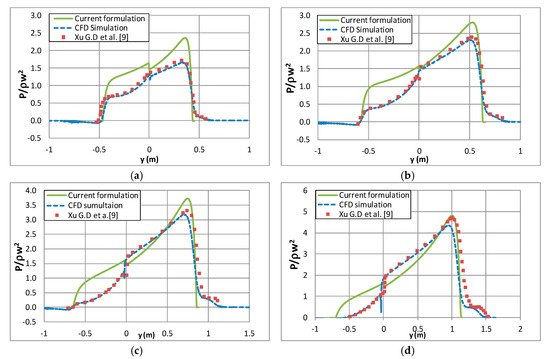
Figure 13.
Pressure distribution with rotational velocity, w = 5 m/s, ω = −2.5 rad/s, β = 45°, Vcg = 0.25 m and ϕ0 = −10°. (a) z0 = 0.3 m. (b) z0 = 0.4 m. (c) z0 = 0.5 m. (d) z0 = 0.6 m.
4.3. Impact with Three Degrees of Freedom
Figure 14 shows the pressure distribution during impact with three degrees of freedom and forced motion, the results are compared with CFD simulations with good agreement.
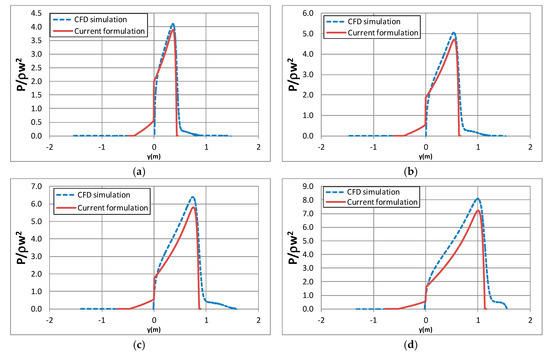
Figure 14.
Pressure distribution during the impact with three degrees of freedom, w = 5 m/s, v = 5 m/s, ω = −2.5 rad/s, β = 45°, Vcg = 0.25 m, and ϕ0 = −10°. (a) z0 = 0.3 m. (b) z0 = 0.4 m. (c) z0 = 0.5 m. (d) z0 = 0.6 m.
4.4. Free Fall Impact
Xu L. et al. [26] performed free fall experiments considering heave and roll. Figure 15 shows the results for the experimental condition β = 20°, B = 0.61 m, A = 2.44 m, M = 124 kg, Vcg = 0.216 m, h = 1.22 m, ϕ0 = 5°, and inertia of section Ixx = 8.85 kg.m2. The results of angular acceleration, vertical acceleration, vertical velocity, and heel angle are shown in Figure 15. The numerical results from the mathematical model have good agreement with CFD simulation and experiments reported by Xu L. et al. [26] in terms of the displacements, velocities, and accelerations.
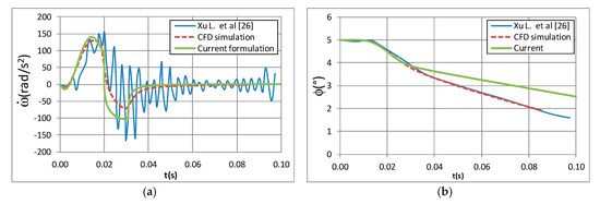
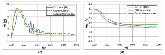
Figure 15.
Free fall impact with two degrees of freedom, m = 124kg, h = 0.61 m, β = 20°, ϕ0 = 5°, Vcg = 0.216 m, and Ixx = 8.85 kg.m2. (a) Angular acceleration during the impact. (b) Heel angle during the impact. (c) Vertical acceleration during the impact. (d) Vertical velocity during the impact.
Impact with three degrees of freedom (heave, sway, and roll) was simulated according to a wedge evaluated by Xu et al. [26]. The test conditions are: β = 20°, B = 0.61 m, A = 2.44 m, m = 124 kg, I = 8.85 kg.m2, Vcg = 0.216 m, h = 0.61 m, and ϕ0 = 5°. Figure 16 shows the results of accelerations and velocities for heave, sway, and roll motions. The results of the mathematical model were compared with CFD simulation and the numerical solution by Wei et al. [10], in terms of the accelerations and velocities. The results show good agreement with the values reported by Wei et al. [10].
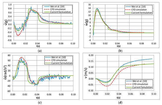
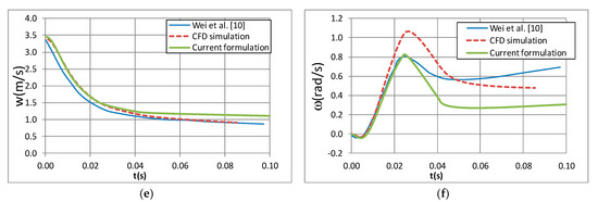
Figure 16.
Impact with three degrees of freedom, m = 293 kg, h = 0.61 m, β = 20°, ϕ0 = 5°, Vcg = 0.216 m, and Ixx = 10.95 kg.m2. (a) Horizontal acceleration during the impact. (b) Vertical acceleration during the impact. (c) Angular acceleration during the impact. (d) Horizontal velocity during the impact. (e) Vertical velocity during the impact. (f) Angular velocity during the impact.
Simulations of the free fall impact with three degrees were performed with a processor Intel I7-4510U CPU@2.00GHz and 6GB RAM memory, the computational time of the current model was 1.83 × 10² s while the CFD simulation with four parallel cores was 2.508 × 10⁵ s. The current model has a low computational cost when compared to CFD.
4.5. Application to Planing Boats
Figure 17 shows the coordinate system used in the study of planing hulls. The system has its origin at the interception of the keel and aft, and it is fixed to the earth. The axis is aligned with the forward velocity. The system is fixed with the boat (BFCS) and rotates with it. The axis is aligned with the keel, while the axis is perpendicular to the symmetry plane of the boat and has its origin at the interception of the keel and aft. The system is fixed to the boat and has its origin in the CG of the boat. The axis is parallel to the keel.
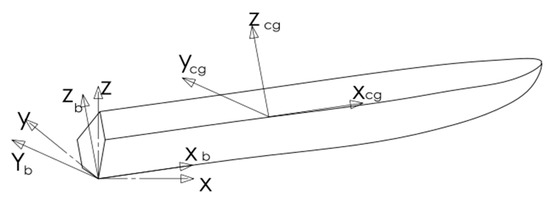
Figure 17.
Boat coordinate systems.
Figure 18 shows a planing boat sailing in steady condition, the boat has a total velocity , trim angle , heel angle and drift angle , and are longitudinal and vertical position respect to the system and is the length of the boat.
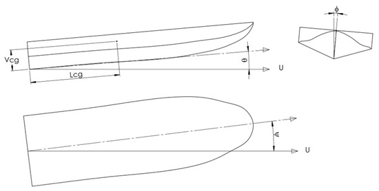
Figure 18.
Steady condition boat.
The results for two-dimensional impact can be used to study the dynamics of a planing boat through the application of slender body theory. The pressure in the hull is computed as:
where is the material derivative of the potential flow function from Equation (29). The velocity for each section of the hull is evaluated as:
where is the vertical velocity of the boat section, is the horizontal velocity of the boat section, is the surge velocity of the boat, is the trim angle, is the pitch velocity, is the yaw velocity, and is the horizontal position of cg from the interception of the keel and aft, including the roll velocity :
The forces over the boat are computed by the integration of the sectional forces along the length. Applying the correction due to aft suction according to Garmé [21]
where , , and are the seccional forces of the boat, and is the correction due to aft suction according to Garmé [21]:
where is the beam of the boat, is the velocity coefficient, and is the position of the section with reference to the interception of the aft and keel. The forces over the boat can be computed as:
where is the force due to viscous drag, is the normal force to the keel and parallel to the water plane, is the normal force to the keel over vertical plane, is the roll moment in the keel, is the trim moment, is the yaw moment evaluated at the interception between the keel and the aft, is the frictional coefficient according to ITTC 1957 [27], is the keel wetted length, and is the wetted area of the hull. The forces in the body fixed coordinate system can be computed as:
where , , , , , and are the forces in the in the body fixed coordinate system at the interception of the aft and keel. The non-dimensional force coefficients are defined as:
where , , and are the non-dimensional forces coefficients in x, y, and z in the body fixed coordinate system. , , , and are the non-dimensional moment coefficients in x, y, and z in the body fixed coordinate system. Brown and Klosinsky [28] carried out towing tank tests in prismatic hulls where the forces in the six degrees of freedom in steady condition were evaluated, during the tests, the forward velocity , trim angle , heel angle and drift angle were varied. Table 2 shows some experimental conditions by Brown and Klosinsky [28], is the wetted keel length. Figure 19 shows the results of roll moment, yaw moment, and drift force as a function of the drift angle which was varied in 0°, 5°, 10°, and 15°. The forces were evaluated for heel angles of 0 and −10°, the values show good agreement with the experimental results reported by Brown and Klosinsky [28].
Table 2.
Experimental conditions by Brown and Klosinsky [28].
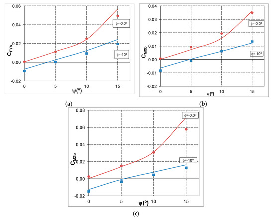
Figure 19.
Forces in planing hulls in steady conditions Cv = 3, β = 20°, and θ = 6°. (a) CFYb vs. Ψ. (b) CMXb vs. Ψ. (c) CMZb vs. Ψ. (―, ―) Current formulation, (•, ▪) Brown and Klosinsky [28].
5. Conclusions
A mathematical model of the impact with three degrees of freedom was developed. The models developed by Wagner [2] and Toyama [3] were extended to study wedge sections considering vertical motion, horizontal motion, and rotation, while the flow separation from the knuckles was evaluated. The pressure distribution and forces were computed during the impact. The model was compared with CFD simulations, experiments, and numerical solutions reported by other authors in the scientific literature, and the results show good agreement. Different impact conditions and degrees of freedom were evaluated, considering forced and free motions. The CFD simulations over predict the forces after the flow separation from the knuckle.
The solution has a low computational cost when compared to commercial CFD software. The model was extended to three dimensions by the application of slender body theory in order to study planing boats in steady conditions. According to the results obtained, and the comparison carried out with different authors and the different conditions considered, this model could be used to study the non-linear dynamics of a planing boat with six degrees of freedom and variable sections along the keel with a low computational cost in comparison with commercial CFD software. The formulation can be used in future works to analyze the seakeeping with cross flow, dynamic stability, maneuverability, pressures, and impact loads over the structure and the crew.
Author Contributions
Conceptualization, R.A. and A.B.; methodology, R.A.; software, A.B.; writing—original draft preparation, R.A. and A.B. All authors have read and agreed to the published version of the manuscript.
Funding
This research received no external funding.
Conflicts of Interest
The authors declare no conflict of interest.
Nomenclature
| deadrise angle of the wedge | |
| deadrise angle in the right side | |
| deadrise angle in the left side | |
| θ | trim angle |
| Ψ | drift angle |
| density of the fluid | |
| potential function of the fluid | |
| heel angle | |
| angular velocity | |
| angular acceleration | |
| μ | asymmetry parameter |
| μ0 | non-dimensional asymmetry parameter |
| asymmetry parameter variation with the time | |
| non-dimensional time | |
| correction factor of the deadrise angle | |
| wetted area of the hull | |
| b | beam section |
| horizontal distance between the keel and knuckle in the right side. | |
| horizontal distance between the keel and knuckle in the left side. | |
| B | beam boat |
| half wetted beam | |
| half wetted beam in the right side. | |
| half wetted beam in the left side | |
| half wetted beam variation in the time | |
| pressure coefficient | |
| frictional coefficient | |
| vertical force coefficient | |
| horizontal force coefficient | |
| roll moment coefficient | |
| velocity coefficient | |
| correction factor for the jet energy | |
| correction due to aft suction | |
| inertia of the wedge | |
| mass of the wedge | |
| horizontal position of cg | |
| keel wetted length | |
| asymmetry ratio | |
| horizontal axis | |
| vertical axis | |
| wedge immersion | |
| hydrostatic horizontal force | |
| hydrostatic vertical force | |
| horizontal force | |
| horizontal sectional force | |
| vertical force | |
| vertical sectional force | |
| roll moment in the keel | |
| hydrostatic roll moment | |
| roll moment in the cg | |
| roll sectional moment | |
| pressure of the fluid | |
| horizontal velocity | |
| horizontal acceleration | |
| tangential velocity in the right side | |
| tangential velocity in the left side | |
| horizontal velocity in the boat section | |
| vertical position of cg | |
| vertical velocity impact | |
| vertical acceleration | |
| vertical velocity in the right side | |
| vertical velocity in the left side | |
| vertical velocity in the boat section | |
| hull force in the x axis on BFCS | |
| hull force in the y axis on BFCS | |
| hull force in the z axis on BFCS | |
| hull moment in the x axis on BFCS | |
| hull moment in the y axis on BFCS | |
| hull moment in the z axis on BFCS | |
| hull force coefficient in the x axis on BFCS | |
| hull force coefficient in the y axis on BFCS | |
| hull force coefficient in the z axis on BFCS | |
| hull moment coefficient in the x axis on BFCS | |
| hull moment coefficient in the y axis on BFCS | |
| hull moment coefficient in the z axis on BFCS |
References
- Ullman Dynamics. Available online: https://ullmandynamics.com/ullman-dynamics-featured-in-ihs-janes-360-a-safe-seat (accessed on 19 December 2019).
- Wagner, H. Über stoss—Und Gleitvorgänge an der Oberfläshe von Flüssigkeiten. Z. Angew. Math. Mech. 1932, 12, 193–215. [Google Scholar] [CrossRef]
- Toyama, Y. Two-dimensional water impact of unsymmetrical bodies. J. Soc. Nav. Arch. Jpn. 1993, 173, 285–291. [Google Scholar] [CrossRef]
- Vorus, W.S. A flat cylinder theory for vessel impact and steady planing resistance. J. Ship Res. 1996, 40, 89–106. [Google Scholar]
- Xu, L.; Troesch, A.; Vorus, W. Asymmetric Vessel Impact and Planing Hydrodynamics. J. Ship Res. 1998, 42, 187–198. [Google Scholar]
- Judge, C.; Troesch, A. Asymmetry and horizontal velocity during water impact. In Proceedings of the International Workshop on Waters Waves and Floating Bodies, Tel Aviv, Israel, 27 February–1 March 2000. [Google Scholar]
- Xu, G.D. Numerical simulation of oblique water entry of an asymmetrical wedge. J. Ocean Eng. 2008, 35, 1597–1603. [Google Scholar] [CrossRef]
- Semenov, Y.A.; Iafrati, A. On the nonlinear water entry problem of asymmetric wedges. J. Fluid Mech. 2006, 547, 231–256. [Google Scholar] [CrossRef]
- Xu, G.D.; Duan, W.Y.; Wu, G.X. Simulation of water entry of a wedge through free fall in three degrees of freedom. Proc. R. Soc. A 2010, 466, 2219–2239. [Google Scholar] [CrossRef]
- Wei, Z.Y.; Xiao, H.Y.; Wang, Z.D.; Shi, X.H. Numerical Simulation of Water Entry of Wedges Based on the Cip Method. J. Mar. Sci. Technol. 2015, 23, 142–150. [Google Scholar]
- Bao, C.M.; Wu, G.X.; Xu, G. Simulation of free fall water entry of a finite wedge with flow detachment. Appl. Ocean Reach. 2017, 65, 62–278. [Google Scholar]
- Seif, M.; Mousaviraad, S.; Saddathosseini, S.; Bertram, V. Numerical Modeling of 2-D Water Impact in One degree of Freedom. Síntesis Tecnológica 2005, 2, 79–83. [Google Scholar] [CrossRef]
- Bilandi, R.; Jamei, S.; Roshan, F.; Azizi, M. Numerical simulation of vertical water impact of asymmetric wedges by using a finite volume method combined with a volume-of-fluid technique. Ocean Eng. 2018, 160, 119–131. [Google Scholar] [CrossRef]
- Tascón, O.; Troesch, A.W.; Maki, K.J. Numerical computation of the hydrodynamic forces acting on a manoeuvring planing hull slender body theory—SBT and 2-D impact theory. In Proceedings of the 10th International Conference on Fast Sea Transportation, Athens, Greece, 5–8 October 2009. [Google Scholar]
- Algarín, R. Modelamiento Del Impacto En Dos Dimensiones De Secciones Asimétricas Con Velocidad Horizontal Con Aplicaciones En El Diseño De Botes De PLANEO. Master’s Thesis, Universidad del Norte, Programa de Ingeniería Mecánica, Barranquilla, Colombia, 2010. [Google Scholar]
- Algarín, R.; Tascón, O. Hydrodynamic Modelling of Planing Boats with Asymmetry and Steady Condition. In Proceedings of the 11th International Symposium on High Speed Marine Vehicle, Naples, Italy, 25–27 May 2011. [Google Scholar]
- Bilandi, R.; Mancini, S.; Vitiello, L.; Miranda, S.; De Carlini, M. A Validation of Symmetric 2D + T Model Based on Single-Stepped Planing Hull Towing Tank Tests. J. Mar. Sci. Eng. 2018, 6, 136. [Google Scholar] [CrossRef]
- Tascón, O.; Algarín, R. Numerical computation of the added mass and damping coefficients of planing hulls in roll via slender body the 2D impact theory. In Proceedings of the 12th International Conference on Fast Sea Transportation, Amsterdam, The Netherland, 2–5 December 2013. [Google Scholar]
- Tavakoli, S.; Dashtimanesh, A.; Mancini, S. A theoretical method to explore influence of free roll motion on behavior of a high speed planing vessel through steady yawed motion. Trans. RINA Int. J. Small Craft Technol. 2018, 160, 25–26. [Google Scholar]
- Zarnick, E.E. A Nonlinear Mathematical Model of Motions of a Planing Boat in Regular Waves, SHIP Performance Department Research and Development Report DTNSRDC-78/032; David, W. Taylor Naval Ship Research and Development Center: Washington, DC, USA, 1978. [Google Scholar]
- Garmé, K. Improved time domain simulation of planing hulls in waves by correction of the near-transom lift. Int. Shipbuild. Prog. 2005, 52, 201–230. [Google Scholar]
- Olausson, K.; Garme, K. Simulation-based assessment of HSC crew exposure to vibration and shock. In Proceedings of the 12th International Conference on Fast Sea Transportation, Amsterdam, The Netherlands, 2–5 December 2013. [Google Scholar]
- ITTC. Recommended Procedures and Guidelines 7.5-03-01. In Uncertainty Analysis in CFD Verification and Validation Methodology and Procedures; 2017; Available online: https://www.ittc.info/media/8153/75-03-01-01.pdf (accessed on 21 November 2019).
- Roache, P.J. Quantification of uncertainty in computational fluid dynamics. Annu. Rev. Fluid Mech. 1997, 29, 123–160. [Google Scholar] [CrossRef]
- Tveitnes, T. Application of Added Mass Theory in Planning. Ph.D. Thesis, Department of Naval Architecture and Ocean Engineering, University of Glasgow, Glasgow, UK, 2001. [Google Scholar]
- Xu, L.; Troesch, A. A study on hydrodynamics of asymmetric planing surfaces. In Proceedings of the 5th International Conference on Fast Sea Transportation, Washington, DC, USA, 31 August–2 September 1999. [Google Scholar]
- ITTC. Concluding technical session. In Proceedings of the 8th International Towing Test Conference, Madrid, Spain, September 1957; Available online: https://ittc.info/media/3089/index.pdf (accessed on 21 November 2019).
- Brown, P.W.; Klosinski, W.E. Directional Stability Tests of Two Prismatic Planing Hulls, Technical Report USCG-D-11-9; Davidson Laboratory, Stevens Institute of Technology Hoboken: Hoboken, NJ, USA, 1994. [Google Scholar]


© 2020 by the authors. Licensee MDPI, Basel, Switzerland. This article is an open access article distributed under the terms and conditions of the Creative Commons Attribution (CC BY) license (http://creativecommons.org/licenses/by/4.0/).