A Density Clustering Algorithm for Simultaneous Modulation Format Identification and OSNR Estimation


Abstract
:1. Introduction
2. Proposed Algorithm: DBSCAN-Based MFI and OSNR Estimation
2.1. Model of MFI and OSNR Estimation Based on DBSCAN Algorithm
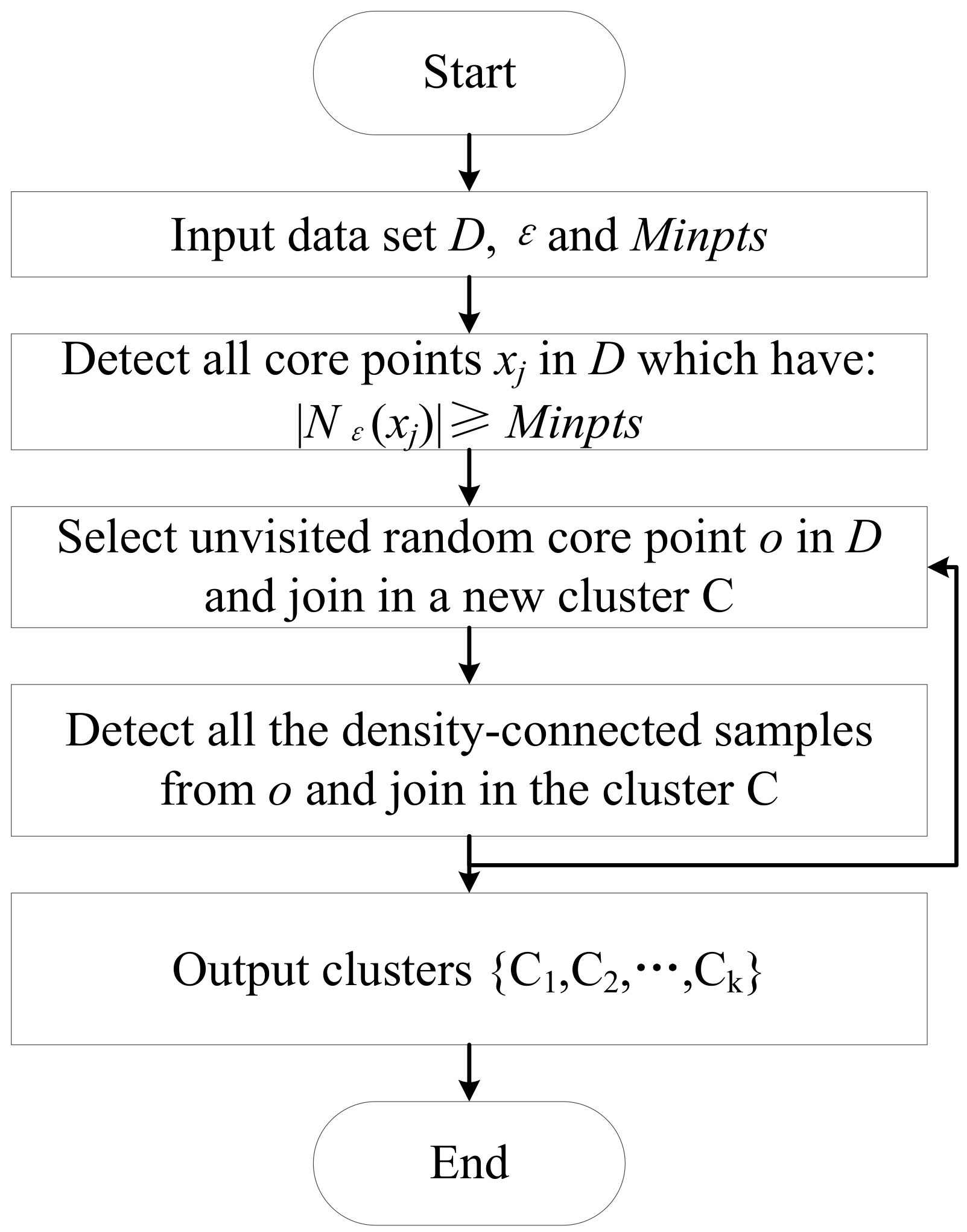
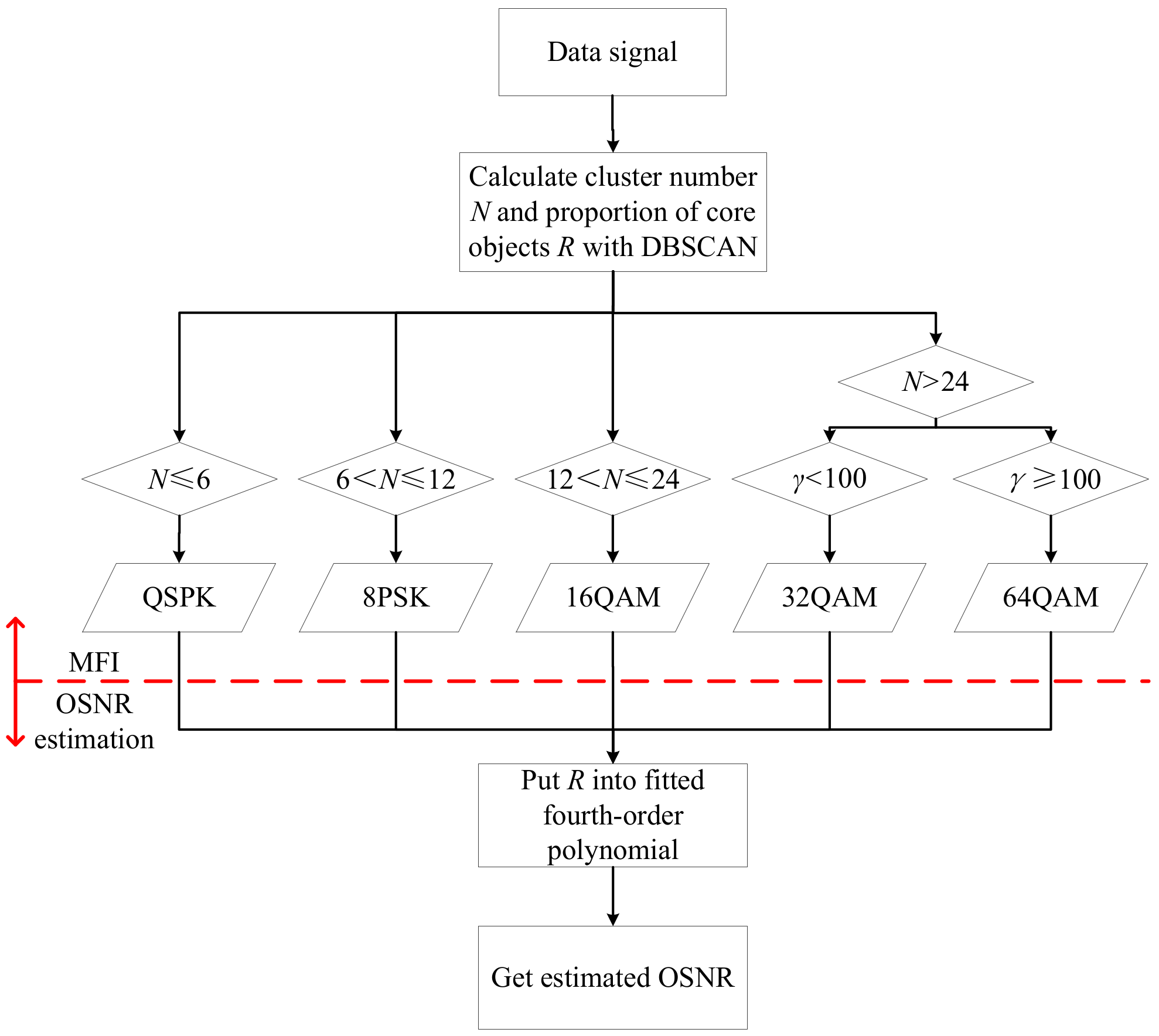
2.2. Flowchart of MFI and OSNR Estimation Based on DBSCAN Algorithm
3. Simulation and Experiment Results
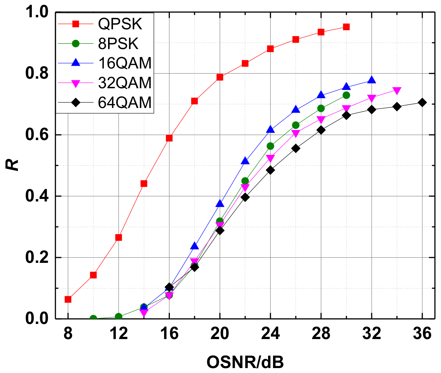
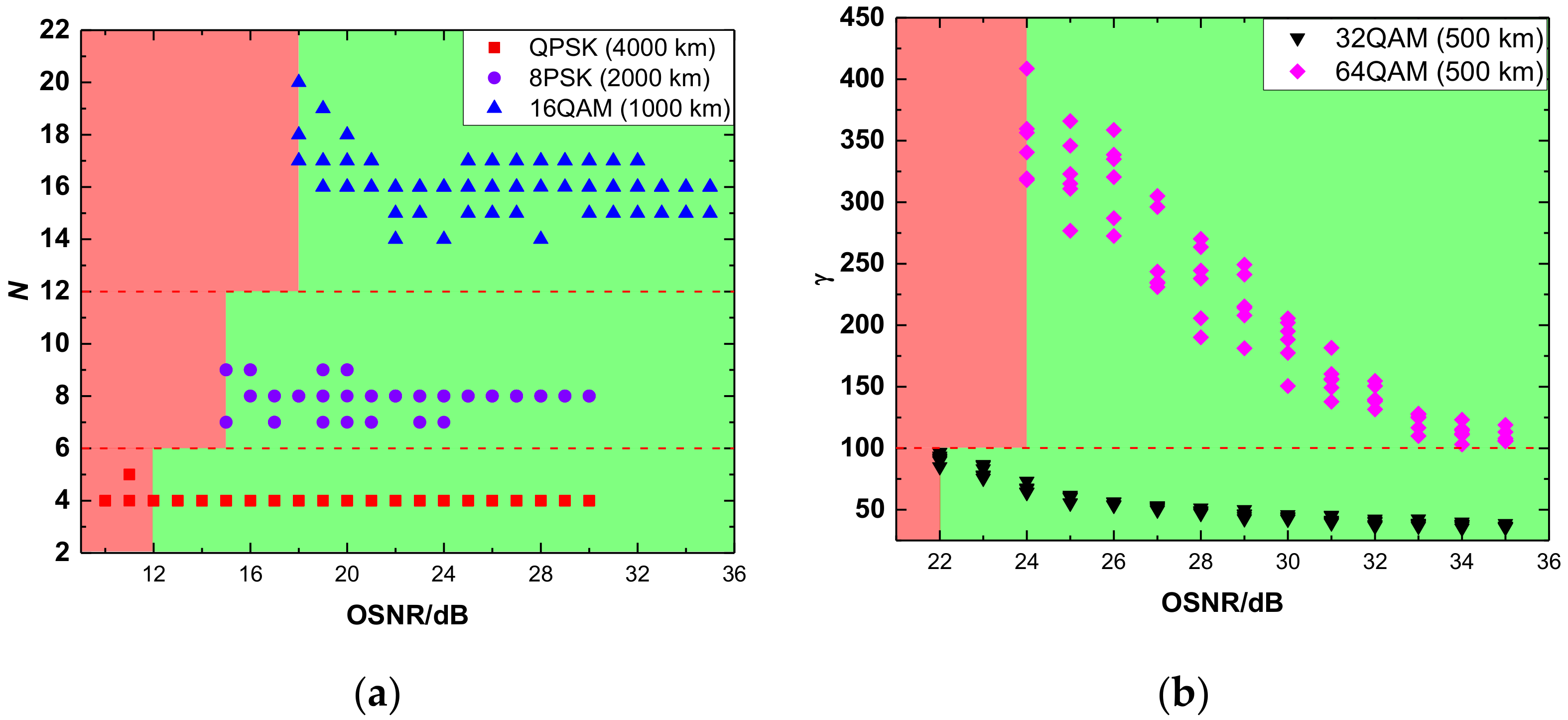
3.1. Simulation Results
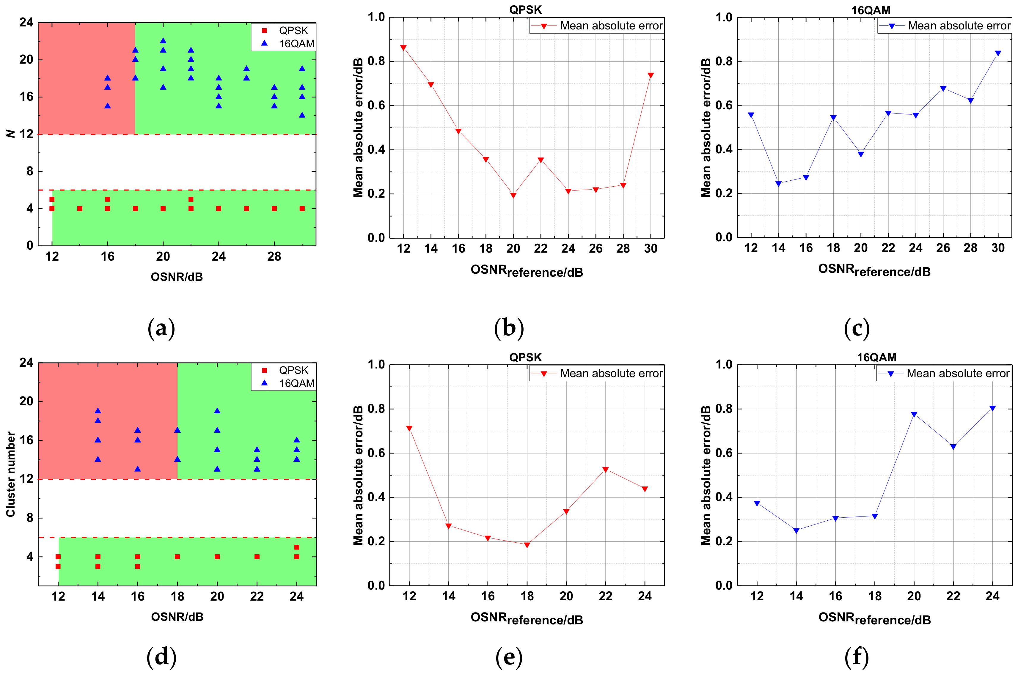
3.2. Results of Proof Experiments
4. Discussion and Conclusions
Author Contributions
Funding
Acknowledgments
Conflicts of Interest
Abbreviations
| ADC | analog-to-digital converter |
| ASE | amplified spontaneous emission |
| AWG | arbitrary waveform generator |
| BER | bit-error ratio |
| CD | chromatic dispersion |
| CMA | constant modulus algorithm |
| DBSCAN | density-based spatial clustering of applications with noise |
| DP | density peaks |
| DSP | digital signal processing |
| EDFA | erbium doped fiber amplifier |
| EON | elastic optical network |
| FEC | forward error correction |
| FO | frequency-offset |
| MF | modulation format |
| MFI | modulation format identification |
| OFDM | orthogonal frequency division multiplexing |
| OPTICS | ordering points to identify the clustering structure |
| OSNR | optical signal-to-noise ratio |
| PDM | polarization division multiplexing |
| PRBS | pseudo-random binary sequence |
| QAM | quadrature amplitude modulation |
| QPSK | quadrature phase shift keying |
| RF | radio frequency |
| SSMF | standard single-mode fiber |
| VOA | variable optical attenuator |
| WDM | wavelength division multiplexing |
Appendix A
- -neighborhood
- Core point
- Directly density-reachable
- Density-reachable
- Density-connected
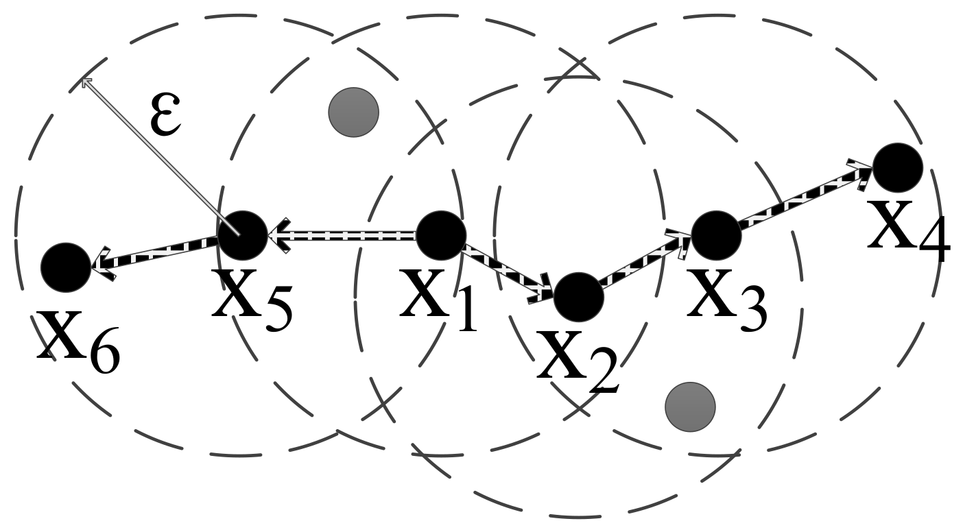
- connectivity: and are density-connected.
- maximality: , and are density-connected .

References
- Gerstel, O.; Jinno, M.; Lord, A.; Ben Yoo, S.J. Elastic Optical Networking: A New Dawn for the Optical Layer? IEEE Commun. Mag. 2012, 50, S12–S20. [Google Scholar]
- Zhao, Z.; Yang, A.Y.; Guo, P. A Modulation Format Identification Method Based on Information Entropy Analysis of Received Optical Communication Signal. IEEE Access 2019, 7, 41492–41497. [Google Scholar]
- Dong, Z.H.; Khan, F.N.; Sui, Q.; Zhong, K.P.; Lu, C.; Lau, A.P.T. Optical Performance Monitoring: A Review of Current and Future Technologies. J. Lightwave Technol. 2016, 34, 525–543. [Google Scholar]
- Khan, F.N.; Lu, C.; Lau, A.P. Optical performance monitoring for fiber-optic communication networks. In Enabling Technologies for High Spectral-Efficiency Coherent Optical Communication Networks; Wiley: Hoboken, NJ, USA, 2016. [Google Scholar]
- Savory, S.J. Digital Coherent Optical Receivers: Algorithms and Subsystems. IEEE J. Sel. Top. Quantum Electron. 2010, 16, 1164–1179. [Google Scholar]
- Willner, A.E.; Pan, Z.; Yu, C. Optical performance monitoring. In Optical Fiber Telecommunications VB; Academic Press: Cambridge, MA, USA, 2008; pp. 233–292. [Google Scholar]
- Swami, A.; Sadler, B.M. Hierarchical digital modulation classification using cumulants. IEEE Trans. Commun. 2000, 48, 416–429. [Google Scholar]
- Liu, J.; Dong, Z.H.; Zhong, K.P.; Lau, A.P.T.; Lu, C.; Lu, Y.Z. Modulation Format Identification Based on Received Signal Power Distributions for Digital Coherent Receivers. In Proceedings of the 2014 Optical Fiber Communications Conference and Exhibition (Ofc), San Francisco, CA, USA, 9–13 March 2014. [Google Scholar]
- Liu, G.C.; Proietti, R.; Zhang, K.Q.; Lu, H.B.; Ben Yoo, S.J. Blind modulation format identification using nonlinear power transformation. Opt. Express 2017, 25, 30895–30904. [Google Scholar]
- Bilal, S.M.; Bosco, G.; Dong, Z.H.; Lau, A.P.T.; Lu, C. Blind modulation format identification for digital coherent receivers. Opt. Express 2015, 23, 26769–26778. [Google Scholar]
- Bo, T.W.; Tang, J.; Chan, C.K. Modulation Format Recognition for Optical Signals Using Connected Component Analysis. IEEE Photonics Technol. Lett. 2017, 29, 11–14. [Google Scholar]
- Mai, X.F.; Liu, J.; Wu, X.; Zhang, Q.; Guo, C.J.; Yang, Y.F.; Li, Z.H. Stokes space modulation format classification based on non-iterative clustering algorithm for coherent optical receivers. Opt. Express 2017, 25, 2038–2050. [Google Scholar]
- Jiang, L.; Yan, L.S.; Yi, A.L.; Pan, Y.; Bo, T.W.; Hao, M.; Pan, W.; Luo, B. Blind Density-Peak-Based Modulation Format Identification for Elastic Optical Networks. J. Lightwave Technol. 2018, 36, 2850–2858. [Google Scholar]
- Chen, P.Y.; Liu, J.; Wu, X.; Zhong, K.P.; Mai, X.F. Subtraction-Clustering-Based Modulation Format Identification in Stokes Space. IEEE Photonics Technol. Lett. 2017, 29, 1439–1442. [Google Scholar]
- Boada, R.; Borkowski, R.; Monroy, I.T. Clustering algorithms for Stokes space modulation format recognition. Opt. Express 2015, 23, 15521–15531. [Google Scholar]
- Wang, D.S.; Zhang, M.; Fu, M.X.; Cai, Z.L.; Li, Z.; Han, H.H.; Cui, Y.; Luo, B. Nonlinearity Mitigation Using a Machine Learning Detector Based on k-Nearest Neighbors. IEEE Photonics Technol. Lett. 2016, 28, 2102–2105. [Google Scholar]
- Guesmi, L.; Ragheb, A.M.; Fathallah, H.; Menif, M. Experimental Demonstration of Simultaneous Modulation Format/Symbol Rate Identification and Optical Performance Monitoring for Coherent Optical Systems. J. Lightwave Technol. 2018, 36, 2230–2239. [Google Scholar]
- Zhang, S.T.; Peng, Y.Q.; Sui, Q.; Li, J.P.; Li, Z.H. Modulation format identification in heterogeneous fiber-optic networks using artificial neural networks and genetic algorithms. Photonic Netw. Commun. 2016, 32, 246–252. [Google Scholar]
- Khan, F.N.; Zhong, K.P.; Al-Arashi, W.H.; Yu, C.Y.; Lu, C.; Lau, A.P.T. Modulation Format Identification in Coherent Receivers Using Deep Machine Learning. IEEE Photonics Technol. Lett. 2016, 28, 1886–1889. [Google Scholar]
- Faruk, M.S.; Mori, Y.; Kikuchi, K. In-Band Estimation of Optical Signal-to-Noise Ratio from Equalized Signals in Digital Coherent Receivers. IEEE Photonics J. 2014, 6, 7800109. [Google Scholar]
- Schmogrow, R.; Nebendahl, B.; Winter, M.; Josten, A.; Hillerkuss, D.; Koenig, S.; Meyer, J.; Dreschmann, M.; Huebner, M.; Koos, C.; et al. Error Vector Magnitude as a Performance Measure for Advanced Modulation Formats. IEEE Photonics Technol. Lett. 2012, 24, 61–63. [Google Scholar]
- Chitgarha, M.R.; Khaleghi, S.; Daab, W.; Almaiman, A.; Ziyadi, M.; Mohajerin-Ariaei, A.; Rogawski, D.; Tur, M.; Touch, J.D.; Vusirikala, V.; et al. Demonstration of in-service wavelength division multiplexing optical-signal-to-noise ratio performance monitoring and operating guidelines for coherent data channels with different modulation formats and various baud rates. Opt. Lett. 2014, 39, 1605–1608. [Google Scholar]
- Ahsan, A.S.; Wang, M.S.; Chitgarha, M.R. Autonomous OSNR monitoring and cross-layer control in a mixed bit-rate and modulation format system using pilot tones. In Photonic Networks and Devices; Optical Society of America: Washington, DC, USA, 2014; p. NT4C. 3. [Google Scholar]
- Lundberg, L.; Sunnerud, H.; Johannisson, P. In-Band OSNR Monitoring of PM-QPSK Using the Stokes Parameters. In Proceedings of the 2015 Optical Fiber Communications Conference and Exhibition (Ofc), Los Angeles, CA, USA, 22–26 March 2015. [Google Scholar]
- Do, C.; Tran, A.V.; Zhu, C.; Hewitt, D.; Skafidas, E. Data-Aided OSNR Estimation for QPSK and 16-QAM Coherent Optical System. IEEE Photonics J. 2013, 5, 6601609. [Google Scholar]
- Oda, S.; Yang, J.Y.; Akasaka, Y. In-band OSNR monitor using an optical bandpass filter and optical power measurements for super channel signals. In Proceedings of the 39th European Conference and Exhibition on Optical Communication (ECOC 2013), London, UK, 22–26 September 2013. [Google Scholar]
- Shen, T.S.R.; Sui, Q.; Lau, A.P.T. OSNR Monitoring for PM-QPSK Systems With Large Inline Chromatic Dispersion Using Artificial Neural Network Technique. IEEE Photonics Technol. Lett. 2012, 24, 1564–1567. [Google Scholar]
- Dong, Z.H.; Lau, A.P.T.; Lu, C. OSNR monitoring for QPSK and 16-QAM systems in presence of fiber nonlinearities for digital coherent receivers. Opt. Express 2012, 20, 19520–19534. [Google Scholar]
- Khan, F.N.; Zhong, K.P.; Zhou, X.; Al-Arashi, W.H.; Yu, C.Y.; Lu, C.; Lau, A.P.T. Joint OSNR monitoring and modulation format identification in digital coherent receivers using deep neural networks. Opt. Express 2017, 25, 17767–17776. [Google Scholar]
- Wang, D.S.; Zhang, M.; Li, J.; Li, Z.; Li, J.Q.; Song, C.; Chen, X. Intelligent constellation diagram analyzer using convolutional neural network-based deep learning. Opt. Express 2017, 25, 17150–17166. [Google Scholar]
- Rodriguez, A.; Laio, A. Clustering by fast search and find of density peaks. Science 2014, 344, 1492–1496. [Google Scholar]
- Mehmood, R.; Zhang, G.Z.; Bie, R.F.; Dawood, H.; Ahmad, H. Clustering by fast search and find of density peaks via heat diffusion. Neurocomputing 2016, 208, 210–217. [Google Scholar]
- Wang, S.L.; Wang, D.K.; Li, C.Y.; Li, Y.; Ding, G.Y. Clustering by Fast Search and Find of Density Peaks with Data Field. Chin. J. Electron. 2016, 25, 397–402. [Google Scholar]
- Ankerst, M.; Breunig, M.M.; Kriegel, H.P.; Sander, J. OPTICS: Ordering points to identify the clustering structure. ACM Sigmod Rec. 1999, 28, 49–60. [Google Scholar]
- Jajoo, G.; Kumar, Y.; Yadav, S.K.; Adhikari, B.; Kumar, A. Blind signal modulation recognition through clustering analysis of constellation signature. Expert Syst. Appl. 2017, 90, 13–22. [Google Scholar]
- Agrawal, K.P.; Garg, S.; Sharma, S.; Patel, P. Development and validation of OPTICS based spatio-temporal clustering technique. Inf. Sci. 2016, 369, 388–401. [Google Scholar]
- Gungor, E.; Ozmen, A. Distance and density based clustering algorithm using Gaussian kernel. Expert Syst. Appl. 2017, 69, 10–20. [Google Scholar]
- Ester, M.; Kriegel, H.P.; Sander, J.; Xu, X.A. Density-based algorithm for discovering clusters in large spatial databases with noise. Kdd 1996, 96, 226–231. [Google Scholar]
- Schubert, E.; Sander, J.; Ester, M.; Kriegel, H.P.; Xu, X.W. DBSCAN Revisited, Revisited: Why and How You Should (Still) Use DBSCAN. ACM Trans. Database Syst. 2017, 42, 1–21. [Google Scholar]
- Kumar, K.M.; Reddy, A.R.M. A fast DBSCAN clustering algorithm by accelerating neighbor searching using Groups method. Pattern Recognit. 2016, 58, 39–48. [Google Scholar]
- Shen, J.; Hao, X.; Liang, Z.; Liu, Y.; Wang, W.; Shao, L. Real-time superpixel segmentation by DBSCAN clustering algorithm. IEEE Trans. Image Process. 2016, 25, 5933–5942. [Google Scholar]
- Czerniawski, T.; Sankaran, B.; Nahangi, M.; Haas, C.; Leite, F. 6D DBSCAN-based segmentation of building point clouds for planar object classification. Autom. Constr. 2018, 88, 44–58. [Google Scholar]
- Tan, Q.Z.; Yang, A.Y.; Guo, P. Blind Modulation Format Identification Using Differential Phase and Amplitude Ratio. IEEE Photonics J. 2019, 11, 7201312. [Google Scholar]
- Tan, Q.Z.; Yang, A.Y.; Guo, P. Blind Modulation Format Identification Using the DC Component. IEEE Photonics J. 2019, 11, 7902910. [Google Scholar]
- Wang, Z.Y.; Yang, A.Y.; Guo, P.; He, P.J. OSNR and nonlinear noise power estimation for optical fiber communication systems using LSTM based deep learning technique. Opt. Express 2018, 26, 21346–21357. [Google Scholar]


| Modulation Format | ||
|---|---|---|
| QPSK | 0.05 | 23 |
| 8PSK | 0.09 | 25 |
| 16QAM | 0.07 | 22 |
| 32QAM | 0.1 | 26 |
| 64QAM | 0.05 | 24 |
© 2020 by the authors. Licensee MDPI, Basel, Switzerland. This article is an open access article distributed under the terms and conditions of the Creative Commons Attribution (CC BY) license (http://creativecommons.org/licenses/by/4.0/).
Share and Cite
Zhao, Z.; Yang, A.; Guo, P.; Tan, Q. A Density Clustering Algorithm for Simultaneous Modulation Format Identification and OSNR Estimation. Appl. Sci. 2020, 10, 1095. https://doi.org/10.3390/app10031095
Zhao Z, Yang A, Guo P, Tan Q. A Density Clustering Algorithm for Simultaneous Modulation Format Identification and OSNR Estimation. Applied Sciences. 2020; 10(3):1095. https://doi.org/10.3390/app10031095
Chicago/Turabian StyleZhao, Zhao, Aiying Yang, Peng Guo, and Qingzhao Tan. 2020. "A Density Clustering Algorithm for Simultaneous Modulation Format Identification and OSNR Estimation" Applied Sciences 10, no. 3: 1095. https://doi.org/10.3390/app10031095