Abstract
The cyber processing layer of smart systems based on a cognitive dynamic system (CDS) can be a good solution for better decision making and situation understanding in non-Gaussian and nonlinear environments (NGNLE). The NGNLE situation understanding means deciding between certain known situations in NGNLE to understand the current state condition. Here, we report on a cognitive decision-making (CDM) system inspired by the human brain decision-making. The simple low-complexity algorithmic design of the proposed CDM system can make it suitable for real-time applications. A case study of the implementation of the CDS on a long-haul fiber-optic orthogonal frequency division multiplexing (OFDM) link was performed. An improvement in Q-factor of ~7 dB and an enhancement in data rate efficiency ~43% were achieved using the proposed algorithms. Furthermore, an extra 20% data rate enhancement was obtained by guaranteeing to keep the CDM error automatically under the system threshold. The proposed system can be extended as a general software-based platform for brain-inspired decision making in smart systems in the presence of nonlinearity and non-Gaussian characteristics. Therefore, it can easily upgrade the conventional systems to a smart one for autonomic CDM applications.
1. Introduction
The cognitive dynamic system (CDS) is inspired by the human brain neuroscience model that is built on the principles of cognition based on perception-action cycle (PAC), memory, attention, intelligence, and language [1,2,3]. The basic model of a CDS is provided in Figure 1. Also, Figure 1 shows three main subsystems of CDS: (i) perceptor for sensing the environment, (ii) the feedback channel for sending internal rewards, and (iii) the executive for performing actions on the environment. The CDS cycles through these subsystems which are known as the perception-action cycle. More details about CDS and PAC can be found in [2]. The CDS can be considered as enhanced artificial intelligence (AI). A CDS creates internal rewards and uses it to take some actions, while AI takes actions based on the rewards [2]. The CDS was proposed as an alternative to artificial intelligence in most AI applications [2,3].
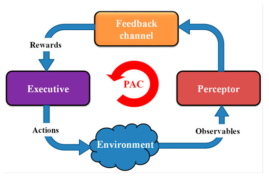
Figure 1.
Block diagram of cognitive dynamic system (CDS).
In [2,3], the CDS was used for cognitive radar applications to provide optimal target detection and intelligent signal processing. In [2,3,4], the CDS was applied for cognitive radio applications, such as dynamic spectrum management in wireless communication networks [4]. The CDS was discussed for theory and applications of cognitive control [3,5]. In [6], the general concept of CDS was introduced for risk control in physical systems. Specific applications of CDS for risk control were presented for vehicular radar transmit waveform selection [7], mitigating the cyber-attack in a smart grid [8], detecting the cyber-attack in smart grid [9], and to mitigate vehicle to vehicle (V2V) jamming [10]. Also, CDS was applied as the brain of complex network [11]. A prospective block diagram of a CDS for smart homes was presented in [12]. In [13], the application of CDS for cybersecurity applications was discussed.
To date, the algorithms of CDS proposed in literature are for linear and Gaussian environments (LGE) [2,3,4,5,6,7,8,9,10,11,12,13]. Here, LGE means that the outputs of the environment linearly depend on the inputs and they have a Gaussian distribution. Therefore, the typical CDS in [2,3,4,5,6,7,8,9,10,11,12,13] uses the Kalman filter. Usually, the Kalman filter, can be applied to linear environments only. The simplified version of Shannon theory is used in [2,3,4,5,6,7,8,9,10,11,12,13] for a Gaussian environment for calculating the entropic state at time n. A typical CDS can use the entropic state at time n as the internal reward. However, Shannon’s entropy equation cannot be simplified for non-Gaussian environment. Therefore, algorithms proposed in the literature for a typical CDS cannot be applied for non-Gaussian and nonlinear environments (NGNLE). Here, NGNLE means that the outputs of the environment are not linearly dependent on the input and do not have a Gaussian distribution.
We should mention here that many AI applications [14,15,16,17,18,19,20] are for NGNLEs. For example, most data obtained or measured from health conditions, education, and social sciences are often not normally distributed [14]. Some examples of non-Gaussian distribution for health conditions, education, and social sciences are prostate cancer modeling [15,16], psychometrics [17], and labor income [18], respectively. The same holds true for a long-haul fiber-optic link as a NGNLE [19,20].
The computational complexity of CDS algorithms in [2,3,4,5,6,7,8,9,10,11,12,13] is high in a complex environment. Also, in an NGNLE, the complexity of CDS algorithms in [2,3,4,5,6,7,8,9,10,11,12,13] is higher than those for a LGE. In this paper, we develop a CDS for NGNLE with simple, straightforward, and faster PAC algorithms.
In [20,21,22], the CDS was proposed for smart fiber optic communication systems as an example of smart systems using cognitive decision-making (CDM). Here, a CDS is used to control the quality of service in long-haul fiber-optic links. The proposed CDS can take some actions such as changing the data rate so that the bit error rate (BER) is under the predefined threshold. In [20], a CDS with a simple executive was presented. The simple executive cannot predict the outcome of the actions before applying actions on the environment. Besides, the simple executive cannot control the modeling configuration of the perceptor or predict the outcome of actions using a virtual environment. In [23], a CDS is presented for NGNLE applications using advanced executive that can predict the outcome of the actions. However, the perceptor in [20,23] can only extract the environment is model without memory. In [24], a CDS was presented for real-time health situation understanding for smart e-Health home applications. Reference [24] uses a perceptor that can extract the model using the adaptive decision-making tree. However, in [24], the executive cannot predict the outcome of actions using virtual actions before applying them on a NGNLE.
In this paper, a general-purpose algorithm for the CDS for a CDM system in a NGNLE with finite memory is presented. The proposed CDS uses an advanced executive that can predict the outcome of multiple actions before applying an action to the environment. In addition, the advanced executive can change the modeling configuration of the perceptor through internal commands. Also, the perceptor can extract the model of a NGNLE with finite memory. In addition, a case study of new CDS and an algorithm are presented for a long-haul fiber-optic link as example of NGNLE. It is demonstrated that this new design can provide ~43% data-rate efficiency enhancement and 7 dB Q-factor improvement. This CDS can replace the typical soft decision forward error correction (SD-FEC) in a fiber optic link and increase the data rate efficiency. To ensure that we have a reliable communications link, the SD-FEC uses 20% overhead (OH) in the optical communications system [25]. However, the typical function of the CDS is to keep the CDM error under the system threshold. A comparison between the proposed method and some related works [20,21,23] for our long-haul fiber optic communications case study is given in Table 1.

Table 1.
Comparison between proposed work and related work published in literature.
The paper is organized as follows. In Section 2, the NGNLE with finite memory is discussed. In Section 3, the architectural structure of CDS and the proposed algorithms CDM for a general NGNLE are presented. In Section 4, we discuss the simulation results for the case study of a long-haul fiber-optic orthogonal frequency division multiplexing (OFDM) link. Finally, in Section 5, we summarize the main contributions of our work.
2. Non-Gaussian and Nonlinear Environment (NGNLE) with Finite Memory
As mentioned before, a NGNLE means that most of the observables (outputs) from the measurement are not linear functions of unknown NGNLE inputs. Also, the observables do not have a Gaussian distribution. In most NGNLE applications, we can measure the observables as the output. However, since the current situation of NGNLE is unknown, we need to decide between M discrete known situations.
Suppose is a vector of variables as a function of discrete time n corresponding to S known discrete states or situations (See Figure 2). For example, in communication systems that uses QAM-4, there are four possible symbols, which vary as a function of time. The receiver may select out of four possible symbols as the symbol that was transmitted at time n. The relation between observables and a NGNLE situation can be defined as follows:
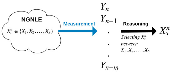
Figure 2.
Decision making between S known situations using m focus levels.
Here, is set of observables that is extracted from measured signals from the sensors (e.g., [26,27]) from discrete time to . Also, m is the current focus level that can be used for the reasoning with acceptable complexity. As mentioned before, corresponds to the current NGNLE condition or situation, which we want to estimate. In (1), is known by measurements or another information gathering technique, but, is unknown. Also, in (1), represents noise with an arbitrary probability density function (PDF), which could be non-Gaussian. The is a nonlinear mapping of and to . One example of such a system can be seen in a long-haul orthogonal frequency division multiplexing fiber optic link. In the next section, we briefly describe the OFDM fiber optic link.
2.1. OFDM-Based Fiber Optic System
OFDM has received significant attention from the researchers in optical communication systems [28,29,30] because high data rate fiber optic links are the backbone of modern communications such as the internet, TV, or medical data transmissions. Figure 3 shows the conventional OFDM-based fiber optic system. The binary data is mapped onto symbols using a symbol mapper that modulate the subcarriers using the inverse fast Fourier transform (IFFT). Usually, a cyclic prefix (CP) can be used in the guard intervals (GI) between OFDM frames to improve distortions due to chromatic dispersion (CD) [30].
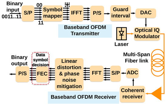
Figure 3.
The conventional orthogonal frequency division multiplexing (OFDM)-based fiber optic system. (ADC: Analog to Digital Converter, DAC: Digital to Analog Converter, FEC: Forward Error Correction, FFT: Fast Fourier Transform, IFFT: Inverse Fast Fourier Transform, P/S: Parallel to Serial, and S/P: Serial to Parallel).
The baseband OFDM data in the digital domain is converted into the optical domain using an optical IQ modulator. After propagating through a long-haul fiber optic link, the coherent receiver [31,32] converts the data into the digital domain. The fast Fourier transform (FFT) demultiplexes the data in orthogonal subcarriers, and then, the signal passes through a linear distortion and phase noise mitigation (LDPNM) block. The LDPNM can adequately compensate for CD and linear distortions. But nonlinear distortions in a fiber optic link cannot be efficiently removed by conventional nonlinear mitigation methods in practical applications. These nonlinear distortions can be deterministic such as self-phase modulation (SPM), cross-phase modulation (XPM), and four-wave mixing (FWM) between subcarriers or stochastic nonlinear impairments such as the interaction between amplified spontaneous emission (ASE) and Kerr effect leading to Gordon–Mollenauer phase noise [33].
2.2. Long-Haul Fiber Optic OFDM Link an Example of NGNLE
Typically, in the analysis of long-haul fiber optic systems, the fiber optic channel is assumed to be nonlinear and the noise is assumed to be Gaussian to simplify the problem [34]. Under the Gaussian noise assumption, it follows that the variance of nonlinear noise should be proportional to the total distance L. However, in [34], it was shown that the variance of nonlinear noise scales as where depending on the dispersion map. Therefore, the Gaussian noise assumption is not accurate for OFDM systems in the presence of nonlinearity. In this paper, we investigate the performance of a long-haul fiber optic OFDM link that is an example of a NGNLE. Figure 4 shows an OFDM system with a CDS. In Figure 4, we assumed that the CDS is placed in the receiver, but the CDS can also send commands to the transmitter, such as changing the data-rate or the transmitted signal power. In addition, the intelligent subsystem of the CDS can be considered as a subsystem of the data symbol decision part of the optical transceiver.
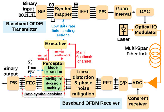
Figure 4.
The OFDM-based fiber optic system enhanced with the CDS.
We should mention here the conventional long-haul fiber optic system uses soft decision (SD) and hard-decision (HD) forward error correction (FEC). This leads to additional overhead to the data rate that reduces the system’s efficiency. Typically, the SD-FEC is used to guarantee the decision-making error before the HD-FEC is under the HD threshold. However, when the CDS is used for decision making as proposed in this paper, it can guarantee that the decision-making error is always under the HD-FEC threshold. Hence, the SD-FEC may no longer be needed when the CDS is used, and therefore, the additional overhead due to SD-FEC could be removed. Figure 3 shows the conventional OFDM-based fiber optic system [28] and Figure 4 shows the upgraded system with the proposed CDS.
3. Why A Cognitive Dynamic System?
In this section, we briefly discuss different machine learning methods. Then, we discuss why CDS is selected among popular machine learning schemes. In this paper, AI uses machine learning approaches to creates intelligent machines. AI created by machine learning is different from symbolic rule-based AI. Therefore, instead of programming predefined rules, AI using machine learning can learn from datasets, examples, and experiences. However, machine learning-based AI requires access to large and reliable datasets, examples, and experiences to provide reliable outcomes. This is an important weakness of machine learning based-AI approaches (including CDS) in comparison to the rule-based AI. Also, this means that the training time is generally longer than rule-based AI. In machine learning-based AI, a machine learning algorithm extracts the model from the dataset. Then, the model can be used for prediction. Also, the algorithm can learn to optimize models based on datasets and policies, for example, in a special task such as providing pre-FEC BER under 0.01 with acceptable modeling complexity.
3.1. Machine Learning Approaches
Machine learning is an interdisciplinary field in computer science, mathematics, and statistics. Generally, there are many machine learning approaches such as supervised learning, reinforcement learning, semi-supervised learning, unsupervised learning, and transfer learning. We will only focus on the first two main types supervised learning and reinforcement learning.
3.1.1. Supervised Learning
In machine learning, a very popular approach for practical applications such as predicting the length of stay in hospital, transmitted symbols in communication systems, radar target detection, or health condition is supervised learning (SL). SL can find patterns inside data. In general, the SL algorithm can learn how to create a classifier for predicting the output variable y for a given input variable x (see Figure 5a). The SL algorithm extracts a mapping function f where y = f(x). An algorithm with a set of data {x1, x2, …, xn} with the corresponding output label {y1, y2, …, yn} builds the classifier.
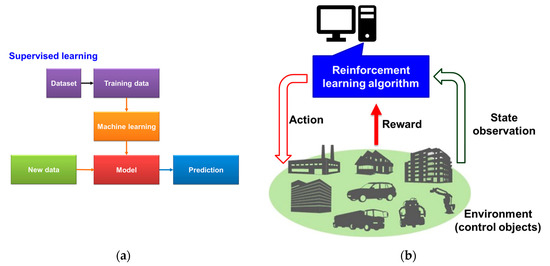
Figure 5.
Schematic of two popular machine learning approaches; (a) supervised learning (SL) and (b) reinforcement learning (RL).
Supervised learning can be divided into two main branches: (1) learning by type of prediction and (2) learning by type of modeling. The type of prediction problems can be divided into regression or classification. For predicting continuous output data, regression learning methods can be more suitable. For the prediction of output class, classification algorithms such as linear regression, naive Bayes, decision trees, or support vector machines (SVM) are better choices [35]. For example, a child’s height prediction is improved with linear regression. However, the decision tree or naive Bayes are better for binary diagnostic test predictions. This type of modeling can be the extraction of a discriminative model such as decision trees and SVM algorithms. These algorithms can extract the decision boundary within the data based on the learning goal. Also, machine learning methods such as naive Bayes or Bayesian approaches, can learn the probability distributions of the data.
In summary, SL trains an algorithm on a labeled database to predict the correct outputs for the unseen inputs. SL can be applied to problems with input/output. In addition, SL can be used for prediction and classification, such as image recognition and filtering spam emails. In this paper we have used the Bayesian approach in CDS perceptor, which is a type of modeling that can extract the posteriori of the data.
3.1.2. Reinforcement Learning
Figure 5b shows a schematic diagram of reinforcement learning (RL). RL maps a decision-making problem into the interaction of a computer agent with a dynamic environment by trial and error [36]. The computer agent attempts to reach the best reward based on feedback received from the dynamic environment when it searches the state and action spaces. For example, in fiber optic communication systems, the RL algorithm will try to improve the model parameters based on iteratively simulating the state (transmitting symbol). Then, after applying the action (e.g., increasing or decreasing data rate and modeling accuracy), the agent obtains the feedback reward from the environment (real transmitted data in transmitter). The RL algorithm can then converge to a model that may generate optimal actions [37].
In summary, RL learns through trial and error from interaction with a dynamic environment such as learning to play a game or a movie/video recommendation system. There are states and actions in RL. Typically, no database is required for RL and it can find that the action for optimizing the reward. But, RL requires that a model be extracted using examples and experiences. RL receives the reward/punishment from the dynamic environment. In this paper, the executive uses RL for applying cognitive actions on a NGNLE (more details provided in the Section 3.2).
3.2. Proposed Cognitive Dynamic System
Figure 6 shows the conceptual implementation of our proposed CDS for the NGNLE (see Figure 7 later). By combining SL and RL as two main approaches of machine learning, CDS can be considered as an enhanced AI. The perceptor of the CDS can extract the model using a SL algorithm. Using the extracted model, the perceptor can generate the internal reward and predict the dynamic environment outcome [3]. In this paper, the dynamic environment is the NGNLE with finite memory (e.g., a long haul OFDM fiber optic link). The perceptor sends the internal reward to the executive through the feedback channel. RL in the executive uses the internal reward in the current PAC to find an action that can decrease/increase the internal reward for the next PAC. But, the proposed CDS can predict the outcome of the actions using a virtual NGNLE to make sure that the action can optimize the internal reward within predefined policy requirements.
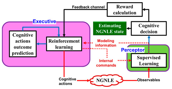
Figure 6.
Conceptual implementation of proposed CDS.
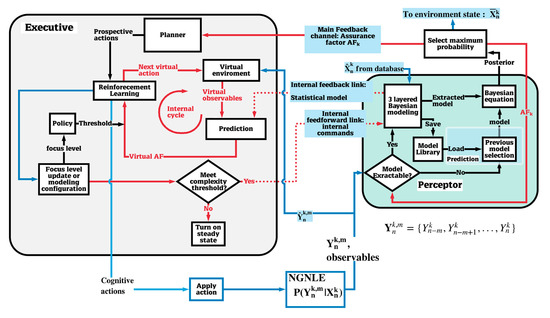
Figure 7.
Architecture of proposed CDS for cognitive decision-making (CDM) in non-Gaussian and nonlinear environments (NGNLE).
In summary, unlike the typical RL, the executive of the CDS can use the extracted model by the perceptor to apply a cognitive action on the dynamic environment. The internal reward gives the CDS self-awareness, self-consciousness, and independence from the dynamic environment. Briefly, the CDS has the “conscience” about the action. For extracting the internal reward, the SL algorithm should be applied in the perceptor. Also, the prediction of cognitive actions outcome is inspired from human brain imagination and risk assessment before doing any action in the real word. However, in a typical RL, the agent applies the actions blindly to receive feedback from the environment. Therefore, the CDS is a more appropriate choice rather than a typical RL in intelligent machine applications.
4. Design of CDS Architecture for Finite Memory NGLNE
The detailed CDS architecture for decision-making is shown in Figure 7. The CDS has two main subsystems: (i) the perceptor and (ii) the executive, with a feedback channel linking them. Through interacting with the environment and shunt cycles, a PAC is created to improve the decision-making accuracy or predictions. The use of local and global feedback loops makes CDS different from artificial intelligence [3]. In this section, we first describe the perceptor and executive using related algorithms when the executive takes actions on the environment, which is followed by changing the focus level when the CDS sends the command to the perceptor as post adaptive actions. The CDS can operate in four modes: (i) pre-adaptive actions mode; (ii) environmental actions mode; (iii) changing the focus level; and (iv) steady state mode. The executive functions will be different depending on the CDS mode, and we will describe them in the following sections. The steady-state mode means that all is well and no more actions are required. Pre-adaptive mode actions are related to finding the first actions to apply on the environment (a typical CDS makes the first action randomly). Mode (ii) is related to actions that can be done on the environment to improve the decision-making accuracy. Also, for improving decision-making accuracy, the CDS can increase the focus level of modeling in the perceptor and learning in the executive in mode (iii). In addition, the CDS can decrease the focus level for the new desired complexity threshold in the mode (iii).
Figure 7 shows that the CDS can use a default database. However, it can be replaced using other techniques in some applications, such as in a long-haul nonlinear fiber optic system (See Section 4 and Figure 4) in which the database is replaced with the estimated data after forward error correction. The perceptor is responsible for knowledge extraction. The knowledge is used to reason and predict the unknown situations for decision-making. The knowledge in the perceptor is represented as a set of concepts and the relationships with the environment situations as described in Section 2. The extracted knowledge can be refined if the CDS increases the focus level. In a specific situation or on user request, the CDS switches from steady state to the pre-adaptive mode. Also, the CDS can dynamically update knowledge in the perceptor and actions library in the executive. Next, the detailed algorithmic descriptions of environmental actions mode (ii) and changing the focus level mode (iii), are presented.
4.1. Perceptor
Conventionally, the perceptor of a CDS should have Bayesian filtering [3]. In this paper, we use the Bayesian equation and the decision-making tree approach for extracting the posterior in decision-making (i.e., ), which is more straightforward than the Bayesian filtering approach. In addition, the multilayer Bayesian generative model using the decision trees concept is a typical method in machine learning. Here, we define m focus levels as the depth of the decision-making tree and i is the arbitrary decision-making node level between zero to m depth levels. This is because we need to design low-complexity and real-time algorithms for NGNLE applications. Therefore, the main sub-blocks of the perceptor are: (i) Bayesian generative model, (ii) previous model selection, and (iii) Bayesian equation and decision-making. The multilayer Bayesian generative model for different focus levels implementation is now presented.
Bayesian Generative Model Extraction
Suppose that there exists no relevant model in a model library. The three-layered Bayesian modeling block extracts the statistical model of the system (see [20,23] for further details) using a decision-making tree. The three-layered Bayesian modeling consists of three layers for an arbitrary focus level of m, as explained in (a), (b), and (c) below:
(a) Layer I:
In a NGNLE, some observables could have any value, and hence, a large number of discretized cells are required for saving vacant spaces. For example, the output of the fiber optic link is a complex variable , where n is the discrete time, k is the PAC number, and m is the current focus level. Therefore, we define the probability box (PB) percentage. The data normalized in this way is sent to Layer II as the for further processing. For the 2D observables, this box can be determined as the and for the minimum and maximum of the probability box in the x-axis together with and for minimum and maximum of the box in the y-axis. The internal reward is used to select the borders of the probabilistic box adaptively as the internal commands by the executive. More details provided on the PB parameters can be found in references [20,21,22,23].
(b) Layer II:
In Layer II, the values related to observables are discretized with discretization steps and which can be two-dimensional if the observables are complex numbers (e.g., see [20,21,22,23]) and . For simplicity, we define a precision factor for each focus level as (assume ):
Here, and are the number of discretized cells in the x-axis and y-axis, respectively. Furthermore, corresponds to the number of decision-making tree branches (see Equations (3) and (5)). It should be noted that the required storage memory increases exponentially with increasing focus levels (see Equation (8)). In addition, the perceptor requires a larger database to extract a reliable model. Therefore, the complexity threshold is predefined based on the available storage memory for saving the model on hard disk or loading the model into RAM. For the desired complexity threshold, the CDS can update the current focus level m, and probability box using Equation (8). Then, Layer II will send the discretized observables and to Layer III (see Equations (2) and (8)).
(c) Layer III:
In this layer, the system estimates the probability of measured observables for a given (usually, this is known from the database), i.e., by approximating it as the probability of (see Equation (9)) for a given , using the Monte–Carlo method. The extracted model in this layer can be called the Bayesian model. This model is saved in the model library for future use. The executive will use the extracted statistical model for prediction by receiving them from the internal feedback to evaluate the actions virtually before applying them on the environment.
4.2. Bayesian Equation and Maximum Posteriori Selection
The posterior can be calculated using the Bayesian equation as follows:
Here, k denotes the PAC number and n means the CDM at time n. The estimated Bayesian generative model and the evidence are extracted in Layer III. The probability can be estimated using the database.
4.2.1. Maximum Posteriori Selection and Assurance Factor
The CDS can save the estimated posterior in the perceptor library after a one-time calculation. We can use the posterior to select that has the maximum probability in each discretized cell as:
where, and is the total number of decision-making situations (see Section 2 and Equation (1)).
4.2.2. Feedback Channel, Assurance Factor, and Internal Rewards
Typically, the CDS uses the Kalman filter and Shannon theory [3] to calculate the entropic state at time n. The technique based on Kalman filter and Shannon theory is applied to a linear and Gaussian environment. However, in a NGNLE, the complexity of using this algorithm is higher than in the LGE. For our application, the algorithm should be simple, straightforward, and fast. Thus, we would like to avoid using extra logarithms, complicated functions, and integrals required in the entropic state calculation associated with Kalman filter. Therefore, here, the internal reward is inspired by the human decision-making approach with lower computational cost. Most of the time, we make the wrong decision when we assure about something whose occurrence is less than 100% (e.g., gambling). Similarly, the CDS makes a decision using Equation (12), and selects the maximum probability using the maximum a posteriori probability (MAP) rule. Therefore, the CDM error is proportional to the assurance of the decision. Consequently, we define the average assurance factor (AF) as:
Here, is an arbitrary time discrete interval to calculate the assurance factor. Also, we calculate the incremental of the assurance factor in the kth PAC using:
where the and are the assurance factors that can be calculated at the (k−1) and kth PAC, respectively. The internal reward, denoted as the , can be defined as the arbitrary function of and and from the function:
where the is an arbitrary function. The can be defined based on the environment type (e.g., the human body or a fiber optic channel) or the perceptor configurations such as desired computational cost or accuracy. The perceptor sends to the executive by the global feedback channel. In addition, the perceptor sends the estimated Bayesian model and evidence through the internal feedback channel (see Figure 7). Also, the perceptor receives the modeling configurations such as (see Equation (4)) through internal feedforward channel that are internal commands from the executive. Here, is the precision factor at the kth PAC and focus level m. Therefore, the executive uses this information and it can find the proper action for applying on NGNLE. Also, for easy reference, we provide a list of the important notations and their meanings in Table 2.
Table 2.
The important notation list used in this paper.
Now, we provide Algorithm 1 to compute environment actions through the global feedback. In this Algorithm, we include several heading comments, so that it is easy to follow.
| Algorithm 1. Environmental actions through the global feedback |
| Input: The observables , focus level m |
| Output: The as the final action in environmental actions mode |
| Initialization: |
| Pre-adaptive actions: |
| Turn steady state mode off, environmental actions on |
| Apply to the environment (such as fiber optic channel) |
| Threshold(M), |
| 1: for k = 1 to K then |
| 2: Take the observable |
| 3: if the model is not available then |
| 4: if k>1 then |
| 5: Predict using |
| 6: Estimate by MAP rule |
| 7: End if |
| 8: Extract the |
| 9: Calculate the posterior |
| 10: Estimate by decision making |
| 11: Else if model is available then |
| 12: Load model, evidence and posterior from perceptor library |
| 13: Estimate by MAP rule |
| 14: End if |
| 15: Send , to the Executive |
| Internal reward |
| 16: Calculate and send it to executive |
| Planning |
| 17: |
| 18: Localize the set of all close actions to ck |
| Learning |
| 19: If actions belong to environmental set then |
| 20: for t = 1 to T then |
| 21: Apply virtually () |
| 22: Calculate |
| 23: Estimate |
| 24: Calculate |
| 25: if and then |
| 26: |
| 27: |
| 28: break for |
| 29: End if |
| 30: End for |
| 31: if then |
| 32: apply to the environment |
| 33: else |
| Policy updating |
| 34: Update |
| Planning update |
| 35: Switch actions type to internal commands |
| 36: Update |
| 37: if then |
| 38: |
| 39: Switch actions type to environmental actions |
| 40: else |
| 41: Turn on steady-state mode |
| 42: End if |
| 43: End if |
| 44: End for |
4.3. Executive
The executive is an essential part of any CDS. It is responsible for improving the decision-making accuracy. This can be done by applying action on the NGNLE. For example, the executive can activate the actuators in the smart home [38,39] or sends the internal commands to the perceptor for changing the modeling configurations such as . The executive provides non-monotonic reasoning to the CDS by using the internal reward and changing its focus level. The executive designed here has three parts (see Figure 7): Planner (it consists of the actions library also), policy, and learning using prediction of the outcome of the virtual action [21,23]. Next, we describe the planner and policy followed by learning using prediction.
4.3.1. Planner and Policy
The planner extracts the set of prospective actions that are already saved in CDS actions library. Also, the planner selects the first action in the first PAC using pre-adaptive actions. In addition, the planner updates the actions type and sends internal commands to update (see Equation (4)) through the internal feedback and feedforward channels (i.e., the shunt cycle).
In this paper, the policy determines the desired goals that the CDS should achieve using the PAC. For example, the goal can be the trade-off between the desired CDM accuracy and the computational cost. Here, for simplicity, we define the CDS goal as the which means the CDS decision making accuracy goal in focus level m for the desired complexity threshold. For example, the can be 10 percent acceptable decision-making error. The can also be five percent acceptable decision-making error, but the cost is increased modeling complexity.
4.3.2. Learning Using Prediction
(a) Executive actions
The actions space in the executive can be classified as the environmental actions and internal CDS commands. Therefore, we define the actions space as follows:
where ck is the action in the current PAC number k and C is set of all possible actions in the actions space.
The posteriori due to the virtual environmental action of (see Table 1) can be predicted virtually using:
Here, and T is a total number of desired virtual actions that the kth model is still valid for predicting the Tth virtual action. Also, in Equation (19), and (see Equations (10) and (11)) are received through the internal feedback from the perceptor. Therefore, the predicted assurance factor can be calculated as:
and
Then, the predicted internal rewards for the desired virtual action can be calculated using Equation (15) as follows:
Therefore, we can find the action that brings the minimum internal reward as:
As a result, the actions to be applied on the environment can be selected as:
Therefore, is the best action to be applied on the environment to improve the decision-making performance. Algorithm 1 shows the outline of the main processes for the global PAC of our CDS. In some applications, the policy may update the for more accuracy (or even higher complexity with acceptable accuracy).
(b) Internal Commands
As mentioned before, some actions apply on the environment and the CDS receives the internal reward through the global PAC using the main feedback channel. However, the actions can be the internal commands such as the increase or decrease the focus level, which is a trade-off between the computational cost and CDM accuracy (see Equations (4), (8), and (16)).
5. CDS Implementation Case Study: OFDM Long-Haul Fiber Optic Communications
Figure 8 shows the CDS architecture block diagram for an OFDM long-haul fiber optic link. As mentioned before, we select the fiber optic link as an example of a NGNLE. In general, can be supplied by a database during a training period. However, the estimated after FEC can be used instead of the database shown in Figure 7 in fiber optic link for model extraction. The bit error rate after forward error correction (FEC) is between 10−15 and 10−12 [34] when the BER before FEC is less than the FEC-threshold. In addition, the decision-making error can be calculated as the BER. Therefore, the BER can be estimated in two ways. First, if the BER is less than the FEC threshold, then the BER after the FEC can be measured and the BER before FEC can be found using extrinsic information transfer (EXIT) chart [25]. If the BER is more than the FEC threshold, we can estimate the BER using 16 or 32 training frames that are used for linear distortion mitigation. The channel estimation and compensation of linear impairments is done using the linear adaptive channel equalizer that uses 16 training frames to mitigate linear distortion [40]. Therefore, the prospective internal reward can be calculated as follows (see Equation (22) and [20,21,22,23]):
where d is 4 Gb/s discretization step for data rate and is an available reference data rate that is set equal to . Also, the implementation of Equations (17)–(19) for a fiber optic communication system is presented in [21,23].
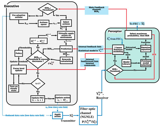
Figure 8.
CDS architecture for long-haul NGNLE OFDM-based fiber optic link.
The actions space for this specific case study is (see Equation (16)):
5.1. Simulations Parameters
We illustrate the modeling process by performing a numerical simulation of an OFDM system (see Figure 8). Signal propagation in an optical fiber is described by the nonlinear Schrödinger equation (NLSE), which is solved using the standard split-step Fourier scheme [34]. The output of the linear equalizer is passed to the perceptor (see Figure 4 and Figure 8). represents the transmitted symbols which takes on the values from the following set with equal probability and represents the corresponding received symbols after linear equalization.
The simulation parameters of the fiber optic system are presented in Table 3. The CDS parameters are as follows: , and 96% probability box. Also, the which is the FEC threshold in focus level zero is 1.03 × 10⁻² (with 14.3% OH for the HD) [41]. Typically, to guarantee reliable communication over a fiber optic link, ~20% SD-FEC overhead is used [25]. However, the CDS can replace the SD-FEC, and with this replacement, the data rate can be enhanced by ~20%. This is because, the CDS (as presented in Algorithm 1) can keep the BER under FEC threshold before HD.
Table 3.
Numerical simulation parameters of the OFDM fiber optic communications system and CDS.
5.2. Simulation Results and Discussions
5.2.1. Pre-Adaptive Actions
The BER of a conventional fiber optic communications system (i.e., without CDS, see Figure 3) is shown in Figure 9. We consider 1.03 × 10⁻² (with 14.3% OH) as the FEC threshold or Threshold (m = 0) for HD [25] (see Table 3). Thus, we can see from Figure 9 that the maximum achievable data rate is 208 Gb/s. The CDS uses 208 Gb/s for j = 1 (i.e., first data rate, = 208 Gb/s). Also, we assume data rate variation by discretization step d = 4 Gb/sand a step of 1 dB for the launch power. Therefore, the data rate for PAC k = 0 is Rref = 204 Gb/s (see Equation (26)). The optimum launch power can be also found using the pre-adaptive method this is already used in the conventional system.
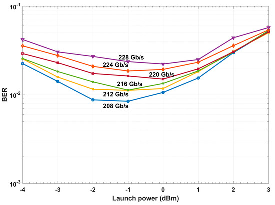
Figure 9.
Bit error rate (BER) for a conventional system with a linear equalizer.
5.2.2. Results for the System with the CDS Focus Level One
The global PAC procedure can be summarized using the results shown in Figure 8, Figure 9, Figure 10, Figure 11, Figure 12, Figure 13 and Figure 14 as follows:
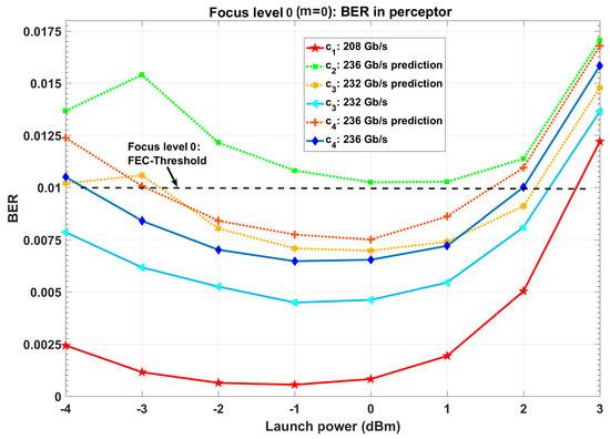
Figure 10.
BER in perceptor after environmental actions (PF = 2, d = 4 Gb/s, focus level zero).
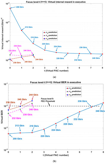
Figure 11.
BER using CDS in executive prediction for virtual actions (PF = 2, d = 4 Gb/s, focus level zero); (a) learning curve for virtual internal reward and (b) virtual BER versus executive internal cycle).
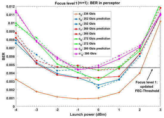
Figure 12.
BER in perceptor after environmental actions (PF = 2, d = 4 Gb/s, focus level one). Dash lines: BER prediction in perceptor and continuous lines: BER using exact model.
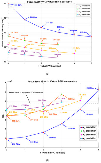
Figure 13.
BER using CDS in executive prediction for virtual actions (PF = 2, d = 4 Gb/s, focus level one); (a) learning curve for virtual internal reward and (b) virtual BER versus executive internal cycle).
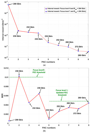
Figure 14.
Results for the CDS versus perception-action cycle (PAC) numbers; (a) CDS learning curve and (b) BER versus PAC numbers.
- First PAC (focus level zero): CDS reduces the date rate to find the first data rate for which the BER is under the FEC-threshold (see Figure 9 and Section 4.2.1). Therefore, 208 Gb/s is applied to the fiber optic link as the first action (c1). Because the BER is under the FEC threshold, the perceptor can extract the statistical model for 208 Gb/s. The perceptor can improve the BER using the extracted model (see Figure 9, c1:208 Gb/s). Note that the minimum BER for a conventional system at 208 Gb/s is (see Figure 9) whereas this is reduced to when the CDS is used (see Figure 10, c1:208 Gb/s). The perceptor sends the extracted model to the executive using the internal feedback link.
- Second PAC (focus level zero): The executive predicts the virtual internal rewards and BER for virtual action of c2 (see Figure 8 and Figure 11 as well as Algorithm 1). Then, the executive applies 236 Gb/s as the c2, because the virtual BER for 240 Gb/s at t = 8 is more than the FEC-threshold of (see Figure 11b, c2: prediction). Also, 236 Gb/s has the minimum virtual internal rewards (See Figure 11a, c2: prediction) and at this data rate, the BER is under FEC threshold (See Figure 11b, c2: prediction). After applying c2 by the CDS (i.e., transmitter sends the data at 236 Gb/s), the perceptor uses the 208 Gb/s model (see Figure 8 and Algorithm 1, previous model selection) to predict the BER for 236 Gb/s. However, the BER is more than FEC-threshold (see Figure 10, c2: 236 Gb/s prediction, topmost curve). Note that we used the previous model selection in this case study. By using previous model selection, the system does not need to transmit the training frames for model extraction.
- Third PAC (focus level zero): The BER is more than the FEC-threshold for c2. Therefore, the executive reduces the data rate by d = 4 Gb/s (see Figure 11). As a result, executive applies 232 Gb/s as c3 in third PAC number. Then, the perceptor uses 208 Gb/s model for BER estimation of 232 Gb/s (See Figure 10, c3: 232 Gb/s prediction) and it can bring the BER for 232 Gb/s under the FEC-threshold. Therefore, the perceptor can extract the model for 232 Gb/s. The extracted model results in further BER improvement for 232 Gb/s (see Figure 10, c3: 232 Gb/s).
- Fourth PAC (focus level zero): The executive applies the 236 Gb/s (See Figure 11, c4: prediction) as c4 to the environment (i.e., fiber optic link) because the predicted BER for 240 Gb/s is more than the FEC-threshold (see Figure 11b, c4: prediction) and virtual internal reward increases for 240 Gb/s (see Figure 11a, c4: prediction). Figure 10 (c4: 236 Gb/s prediction) shows that the perceptor provides the BER for 236 Gb/s under FEC-threshold using the model for 232 Gb/s (provided that the model for 208 Gb/s was used and BER was higher than FEC threshold in second PAC). Like the third PAC, the BER can improve further using the exact extracted model (see Figure 10, c4: 236 Gb/s).
- Fifth PAC (focus level zero and focus level one): The executive finds that the predicted BER for 240 Gb/s is just less than the FEC threshold (see Figure 11b, c5: prediction), but the virtual internal reward increases in comparison to 236 Gb/s (see Figure 11a, c5: prediction). Therefore, the executive updates policy and FEC threshold or . Then, the executive sends the new policy () and the internal command (increasing focus level) to the perceptor. Using, the model extracted in focus level one, the perceptor provides the BER under updated FEC threshold (see Figure 12, c5: 236 Gb/s and Figure 14b). Also, the internal rewards decreased correspondingly (see Figure 14a).
- Sixth PAC (focus level one): The executive predicts the virtual internal rewards and the BER for virtual action of c6 using extended model in focus level 1 (see Figure 12, Figure 13, and Algorithm 1). The executive applies 252 Gb/s as the c6, because the virtual BER for 256 Gb/s at t = 5 is more than the updated FEC-threshold (see Figure 13b, c6: prediction) and the 252 Gb/s has the minimum virtual internal rewards (See Figure 13a, c6: prediction) with virtual BER under updated FEC threshold (See Figure 13b, c6: prediction). After applying c6 by the CDS, the perceptor uses 236 Gb/s extracted model (see Figure 12, c6: 252 Gb/s prediction) to predict the BER for 252 Gb/s. Figure 12 shows that the perceptor provides the BER for 252 Gb/s under the updated FEC-threshold using the extracted model for 236 Gb/s. Similar to previous PAC, the BER can be improved further using the exact extracted model (see Figure 12, c6: 252 Gb/s).
- Seventh, eighth and ninth PAC (focus level one): Similar to sixth PAC, the CDS can provide 260 Gb/s, 272 Gb/s, and 280 Gb/s for the c7, c8, and c9, respectively.
- 10th PAC (focus level one): The executive finds that the predicted BER for 284 Gb/s is more than the updated FEC threshold (see Figure 13b). As a result, the executive turns on steady state for 280 Gb/s. The CDS does not increase the focus level, because the number of cells in the focus level two is more than the desired complexity threshold (see Table 3 for ).
From Figure 12 and Figure 14b, we see that the CDS provides the minimum BER of before HD-FEC, when the data rate is 280 Gb/s (see Figure 12 and Figure 14b). Based on [25], the required OH can be reduced to 6.25%. As a result, an extra ~24 Gb/s in 280 Gb/s data rate can be used for data transmission instead of assigning it for overhead.
5.2.3. CDS Learning Curve
The CDS learning curve is shown in Figure 14a and corresponding BER is shown in Figure 14b. In Figure 14, the PACs 1, 2, 3, and 4 correspond to focus level 0 actions which correspond to the data rate of 208, 236, 232, and 236 Gb/s, respectively (see Algorithm 1). The PACs 5, 6, 7, 8, and 9 are the CDS focus level 1 actions as data rates of 236, 252, 260, 272, and 280 Gb/s, respectively.
The results for the CDS at steady state are summarized in Table 4. The smart fiber optic link that used the focus level concept enhances the data rate efficiency by ~43% in comparison to conventional fiber optic link. This is the summation of ~35% data rate enhancement (i.e., enhancement of the data rate R1 = 208 Gb/s to R9 = 280 Gb/s) and 8% of HD overhead reduction (~24 Gb/s can be used for data carrying, instead of overhead redundancy) reduction, which is achieved by lowering the FEC threshold from to . The final Q-factor improvement is 7 dB, which is a significant improvement for the long-haul fiber optic link. The reason for such significant improvement is that the fiber optic channel using memory and the focus level concept can model the fiber optic channel more accurately in comparison to a memoryless fiber optic link channel. Under the same conditions, the performance improvement using the digital backpropagation (DBP) method is typically 1–2 dB [42] and the computational cost and complexity is significantly higher compared to our proposed system. In addition, the DBP method does not provide data rate enhancement.
Table 4.
The CDS parameters at steady state.
5.2.4. CDS Complexity for Proof-Concept Case Study on Long-Haul OFDM Fiber Optic Link
In order to calculate the computational cost, we distinguish two types of CDS modes: (i) Modeling extraction mode and (ii) Steady-state mode. The complexity of a CDS varies depending on the perceptor mode. When the CDS operates in the BER improvement mode, the BER converges after N OFDM frames (in simulation N = 28,000) and each frame has D data-carrying subcarriers (From Table 1, it is 126). To create the histogram (i.e., to calculate ) based on the discretized data, we need N × D simple additions (just counting the samples within the tiny surface). To calculate , we need S real multiplications where S is the order of QAM (in our example, S = 16), then, we save the maximum probability for the related QAM alphabet. For simplicity, we assume that the minimum and maximum of the probability box in all focus levels are and , respectively for this proof-of-concept example. As a result, the storage requirement depends on the precision factor. For example, with a of 2 in focus level zero, we need to store a matrix of dimension = 60 × 60 (see, Equations (6) and (7), ). Also, the storage requirement in focus level one with a of 2 and a of 5, we need to store the matrix which has a dimension of = 12 by 12 by 60 by 60 (see, Equations (6) and (7), ). These matrices can be stored in a hard disk and can be loaded into RAM when needed. Therefore, the complexity threshold (here, it is 106) is the predefined maximum available storage for saving in a hard disk or loading into RAM, when needed. When the CDS operates in the steady-state mode, there is no cost associated with model extraction (i.e., to calculate ). Therefore, no multiplication or addition is needed in steady state.
For validating, we need to process 28,000 frames (see Table 3) using digital back propagation (DBP), and this cannot be done using typical processors. Therefore, we assumed the DBP processing the 28,000 frames as ~55 blocks of 512 frames. The computational cost associated with DBP for processing 512 OFDM frames is as follows. In each propagation step, complex multiplications are required where J is the number of samples in time domain. If there are B propagation steps, the complex multiplication is [43,44]. For example, for a 20-span system, assuming 10 steps per span and with J = 16,384, we need 45,875,200 complex multiplications! Besides, this computation needs to be done continuously for each block of data. Three complex vectors of length J (the total size of 98,304) needs to be stored. In contrast, most of the computational complexity of the CDS is present only when there is a fluctuation in the fiber optic channel. Under steady-state, the computational cost is minimal.
It is useful to compare the complexity of the proposed method in this paper with the DBP method for Q-factor enhancement using the simulation parameters in Table 3 and processing 28,000 OFDM frames. We run both algorithms on a Microsoft Surface-Pro with Intel ® Core ™ i706650U CPU @ 2.20 GHz 2.21 GHz, 16 GB RAM, system type 64-bit Operating System x64-Based processor using MATLAB. For the DBP algorithm [42], the runtime is 2465.8 s, that is ~41 min and 6s. However, this runtime for 9 PACs with the proposed CDS is 792s (~13 min and 12s). In addition, the CDS running time is reduced to 100s for the CDM in steady-state mode. In contrast, the DBP run time will always remain similar for any continuous data stream. We should mention that the CDS can process all 28,000 frames as one block. However, processing 28,000 frames using DBP method is not feasible using Microsoft Surface-Pro with Intel ® Core ™ i706650U CPU @ 2.20GHz 2.21 GHz, 16 GB RAM. Therefore, we break the 28,000 frames into ~55 blocks, and the DBP run time of ~41 min was achieved in this way. However, we should mention that processing received 28,000 frames in less than 100s in the steady-state mode makes it a practical solution for almost real-time high-quality data transmission such as real-time high-quality video conferencing.
6. Conclusions
In recent years, some efforts were made to develop intelligent machines using cognitive dynamic system for artificial intelligence applications. However, currently, CDS high complexity algorithms available are only applied to LGE. These algorithms cannot be applied for a non-Gaussian and nonlinear environment with finite memory. Therefore, we proposed novel CDS algorithms that could be applied on a NGNLE with finite memory. We redesigned the CDS in detail to make it suitable for NGNLE cognitive decision making applications. Also, the system architecture and algorithms are presented. The proposed algorithm is applied on a long-haul nonlinear fiber-optic link as a case study. By upgrading the conventional link with the CDS, the applicable data-rate increased from 208 Gb/s to 280 Gb/s. Also, the CDS Q-factor improved by ~7 dB (the optimum BER = for 280 Gb/s with CDS). The data rate enhancement is ~35% without considering the HD overhead reduction. However, the CDS brings the BER under the new FEC threshold (=), we do not need 8% of the HD-FEC overhead. Hence, the net data rate enhancement is ~43%. Typically, SD-FEC with as overhead of ~20% is used to guarantee that the BER is under the HD-FEC threshold. An additional advantage of the CDS is that SD-FEC overhead is no longer needed since the CDS tries to keep the BER under the HD-FEC threshold automatically.
Finally, the presented algorithms in this paper are simple and fast because it used the Bayesian equation for calculating the posterior that has low complexity for the calculation. Therefore, the low complexity algorithms make the proposed CDS a perfect candidate for the NGNLE applications such as long-haul fiber optic links or in healthcare.
Author Contributions
All authors contribute equally for writing this paper. All authors have read and agreed to the published version of the manuscript.
Acknowledgments
We would thank Natural Sciences and Engineering Research Council (NSERC) and Canada Research Chair Program (CRCP) for supporting this research work.
Conflicts of Interest
The authors declare no conflict of interest.
References
- Fuster, J.M. Cortex and Mind: Unifying Cognition; Oxford University: Oxford, UK, 2003. [Google Scholar]
- Haykin, S. Cognitive Dynamic Systems: Perception-Action Cycle, Radar, and Radio; Cambridge University: Cambridge, UK, 2012. [Google Scholar]
- Haykin, S. Cognitive Dynamic Systems: Radar, Control, and Radio. Proc. IEEE 2012, 100, 2095–2103. [Google Scholar] [CrossRef]
- Khozeimeh, F.; Haykin, S. Brain-Inspired Dynamic Spectrum Management for Cognitive Radio Ad Hoc Networks. IEEE Trans. Wirel. Commun. 2012, 11, 3509–3517. [Google Scholar] [CrossRef]
- Fatemi, M.; Haykin, S. Cognitive Control: Theory and Application. IEEE Access 2014, 2, 698–710. [Google Scholar] [CrossRef]
- Haykin, S. The Cognitive Dynamic System for Risk Control. Proc. IEEE 2017, 105, 1470–1473. [Google Scholar] [CrossRef]
- Feng, S.; Haykin, S. Cognitive Risk Control for Transmit-Waveform Selection in Vehicular Radar Systems. IEEE Trans. Veh. Technol. 2018, 67, 9542–9556. [Google Scholar] [CrossRef]
- Oozeer, M.I.; Haykin, S. Cognitive Risk Control for Mitigating Cyber-Attack in Smart Grid. IEEE Access 2019, 7, 125806–125826. [Google Scholar] [CrossRef]
- Oozeer, M.I.; Haykin, S. Cognitive Dynamic System for Control and Cyber-Attack Detection in Smart Grid. IEEE Access 2019, 7, 78320–78335. [Google Scholar] [CrossRef]
- Feng, S.; Haykin, S. Cognitive Risk Control for Anti-Jamming V2V Communications in Autonomous Vehicle Networks. IEEE Trans. Veh. Technol. 2019, 68, 9920–9934. [Google Scholar] [CrossRef]
- Fatemi, M.; Setoodeh, P.; Haykin, S. Observability of stochastic complex networks under the supervision of cognitive dynamic systems. J. Complex Netw. 2017, 5, 433–460. [Google Scholar] [CrossRef]
- Feng, S.; Setoodeh, P.; Haykin, S. Smart Home: Cognitive Interactive People-Centric Internet of Things. IEEE Commun. Mag. 2017, 55, 34–39. [Google Scholar] [CrossRef]
- Haykin, S. Artificial Intelligence Communicates with Cognitive Dynamic System for Cybersecurity. IEEE Trans. Cogn. Commun. Netw. 2019, 5, 463–475. [Google Scholar] [CrossRef]
- Bono, R.; Blanca, M.J.; Arnau, J.; Gómez-Benito, J. Non-normal Distributions Commonly Used in Health, Education, and Social Sciences: A Systematic Review. Front. Psychol. 2017, 8, 1602. [Google Scholar] [CrossRef] [PubMed]
- Si, Y.; Liu, R.B. Diagnostic Performance of Monoexponential DWI Versus Diffusion Kurtosis Imaging in Prostate Cancer: A Systematic Review and Meta-Analysis. Am. J. Roentgenol. 2018, 211, 358–368. [Google Scholar] [CrossRef] [PubMed]
- Maurer, M.H.; Heverhagen, J.T. Diffusion weighted imaging of the prostate-principles, application, and advances. Transl. Androl. Urol. 2017, 6, 490–498. [Google Scholar] [CrossRef] [PubMed]
- Micceri, T. The unicorn, the normal curve, and other improbable creatures. Psychol. Bull. 1989, 105, 156–166. [Google Scholar] [CrossRef]
- Diaz-Serrano, L. Labor income uncertainty, skewness and homeownership: A panel data study for Germany and Spain. J. Urban Econ. 2005, 58, 156–176. [Google Scholar] [CrossRef]
- Shahi, S.N.; Kumar, S.; Liang, X. Analytical modeling of cross-phase modulation in coherent fiber-optic system. Opt. Express 2014, 22, 1426–1439. [Google Scholar] [CrossRef]
- Naghshvarianjahromi, M.; Kumar, S.; Deen, M.J. Brain Inspired Dynamic System for the Quality of Service Control Over the Long-Haul Nonlinear Fiber-Optic Link. Sensors 2019, 19, 2175. [Google Scholar] [CrossRef]
- Naghshvarianjahromi, M.; Kumar, S.; Deen, M.J. Cognitive decision making for the long-haul fiber optic communication systems. In Proceedings of the 2019 16th Canadian Workshop on Information Theory (CWIT), Hamilton, ON, Canada, 2–5 June 2019; pp. 1–5. [Google Scholar]
- Naghshvarianjahromi, M.; Kumar, S.; Deen, M.J. Smart long-haul fiber optic communication systems using brain-like intelligence. In Proceedings of the 2019 16th Canadian Workshop on Information Theory (CWIT), Hamilton, ON, Canada, 2–5 June 2019; pp. 1–6. [Google Scholar]
- Naghshvarianjahromi, M.; Kumar, S.; Deen, M.J. Brain-Inspired Cognitive Decision Making for Nonlinear and Non-Gaussian Environments. IEEE Access 2019, 7, 180910–180922. [Google Scholar] [CrossRef]
- Naghshvarianjahromi, M.; Kumar, S.; Deen, M.J. Brain-Inspired Intelligence for Real-Time Health Situation Understanding in Smart e-Health Home Applications. IEEE Access 2019, 7, 180106–180126. [Google Scholar] [CrossRef]
- Zhang, L.M.; Kschischang, F.R. Staircase Codes With 6% to 33% Overhead. J. Lightwave Technol. 2014, 32, 1999–2002. [Google Scholar] [CrossRef]
- Majumder, S.; Mondal, T.; Deen, M.J. Wearable sensors for remote health monitoring. Sensors 2017, 17, 130. [Google Scholar] [CrossRef] [PubMed]
- Majumder, S.; Mondal, T.; Deen, M.J. Smartphone sensors for health monitoring and diagnosis. Sensors 2019, 19, 2164. [Google Scholar] [CrossRef] [PubMed]
- Jansen, S.L.; Morita, I.; Takeda, N.; Tanaka, H. 20 Gb/s OFDM transmission over 4160-km SSMF enabled by RF-pilot tone phase noise compensation. In Proceedings of the PDP15, NFOEC, Anaheim, CA, USA, 25–29 March 2007. [Google Scholar]
- Du, A.; Schmidt, B.; Lowery, A. Efficient digital backpropagation for PDM-CO-OFDM optical transmission systems. In Proceedings of the OFC/NFOEC, OTuE2, San Diego, CA, USA, 21–25 March 2010. [Google Scholar]
- Peng, W.; Takahashi, H.; Morita, I.; Tsuritani, T. Per-symbol-based DBP approach for PDM-CO-OFDM transmission systems. Opt. Express 2013, 21, 1547–1554. [Google Scholar] [CrossRef] [PubMed]
- Bandyopadhyay, A.; Deen, M.J.; Tarof, L.E.; Clark, W. A simplified approach to time-domain modeling of avalanche photodiodes. IEEE J. Quantum Electron. 1998, 34, 691–699. [Google Scholar] [CrossRef]
- Deen, M.J.; Basu, P.K. Silicon Photonics: Fundamentals and Devices; John Wiley & Sons: New York, NY, USA, 2010. [Google Scholar]
- Gordon, J.P.; Mollenauer, L.F. Phase noise in photonic communications systems using linear amplifiers. Opt. Lett. 1990, 15, 1351–1353. [Google Scholar] [CrossRef]
- Skidin, A.S.; Sidelnikov, O.S.; Fedoruk, M.P.; Turitsyn, S.K. Mitigation of nonlinear transmission effects for OFDM 16-QAM optical signal using adaptive modulation. Opt. Express 2016, 24, 30296–30308. [Google Scholar] [CrossRef]
- Cortes, C.; Vapnik, V. Support-vector networks. Mach. Learn. 1995, 20, 273–297. [Google Scholar] [CrossRef]
- Silver, D.; Huang, A.; Maddison, C.J.; Guez, A.; Sifre, L.; Van Den Driessche, G.; Schrittwieser, J.; Antonoglou, I.; Panneershelvam, V.; Lanctot, M.; et al. Mastering the game of go with deep neural networks and tree search. Nature 2016, 529, 484–489. [Google Scholar] [CrossRef]
- Raghu, A.; Komorowski, M.; Celi, L.A.; Szolovits, P.; Ghassemi, M. Continuous state-space models for optimal sepsis treatment-a deep reinforcement learning approach. In Proceedings of the Machine Learning for Healthcare (MLHC) 2017, Boston, MA, USA, 18–9 August 2017; pp. 1–17. [Google Scholar]
- Majumder, S.; Aghayi, E.; Noferesti, M.; Memarzadeh-Tehran, H.; Mondal, T.; Pang, Z.; Deen, M.J. Smart homes for elderly healthcare—Recent advances and research challenges. Sensors 2017, 17, 2496. [Google Scholar] [CrossRef]
- Deen, M.J. Information and communications technologies for elderly ubiquitous healthcare in a smart home. Pers. Ubiquitous Comput. 2015, 19, 573–599. [Google Scholar] [CrossRef]
- Kumar, S.; Deen, M.J. Fiber Optic Communications: Fundamentals and Applications; John Wiley & Sons: Hoboken, NJ, USA, 2014. [Google Scholar]
- Mizuochi, T.; Miyata, Y.; Kubo, K.; Sugihara, T.; Onohara, K.; Yoshida, H. Progress in soft-decision FEC. In Proceedings of the 2011 Optical Fiber Communication Conference and Exposition and the National Fiber Optic Engineers Conference, Los Angeles, CA, USA, 6–10 March 2011; pp. 1–3. [Google Scholar]
- Liang, X.; Kumar, S. Correlated digital backpropagation based on perturbation theory. Opt. Express 2015, 23, 14655–14665. [Google Scholar] [CrossRef] [PubMed]
- Ip, E.; Kahn, J.M. Compensation of dispersion and nonlinear impairments using digital backpropagation. J. Lightwave Technol. 2008, 26, 3416–3425. [Google Scholar] [CrossRef]
- Mateo, E.; Zhu, L.; Li, G. Impact of XPM and FWM on the digital implementation of impairment compensation for WDM transmission using backward propagation. Opt. Express 2008, 16, 16124–16137. [Google Scholar] [CrossRef] [PubMed]


© 2020 by the authors. Licensee MDPI, Basel, Switzerland. This article is an open access article distributed under the terms and conditions of the Creative Commons Attribution (CC BY) license (http://creativecommons.org/licenses/by/4.0/).