Image Dehazing Based on (CMTnet) Cascaded Multi-scale Convolutional Neural Networks and Efficient Light Estimation Algorithm


Abstract
1. Introduction
2. Background
2.1. Atmospheric Scattering Formation Model
2.2. Convolutional Neural Network CNN (ConvNet)
2.3. Image Dehazing Using CNN Architectures
- Most deep learning-based approaches for image dehazing ignore the accurate estimation of atmospheric light [20,26,28] and set its value empirically, which leads to inaccurate dehazing results because the simplified physical model requires the estimation of both atmospheric light and transmission map.
- The inefficiency presented in Song et al.’s method [29], as mentioned in their conclusion, is because of the redundant computations caused by the additional layer.
- The majority of deep learning-based dehazing models lack the structural integrity of the original scene. This trouble produces impractical results far from clear ground truth images when compared to using a structural similarity metric.
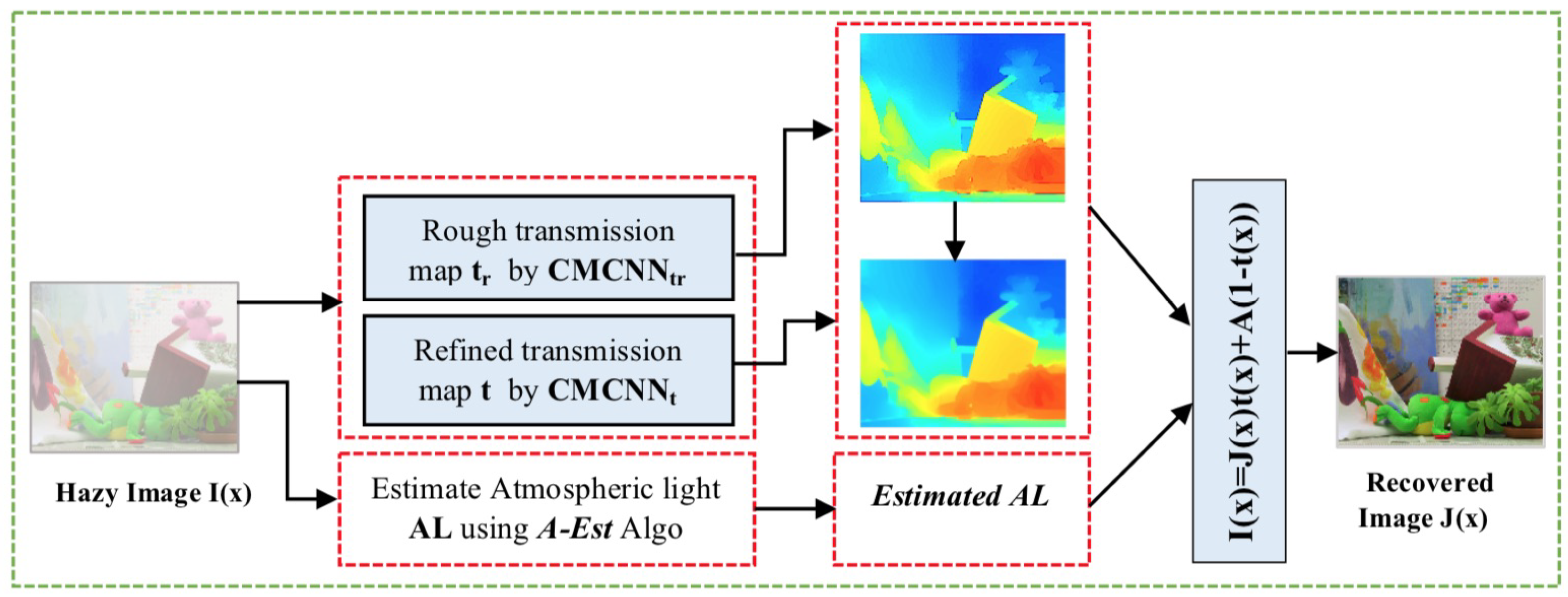
3. Proposed Dehazing Method
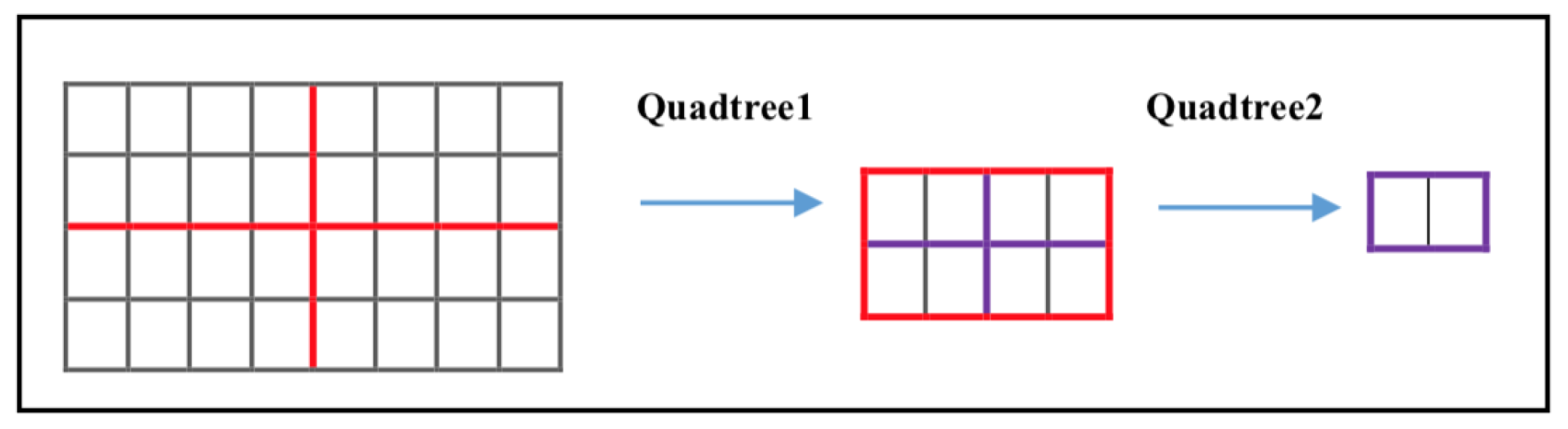
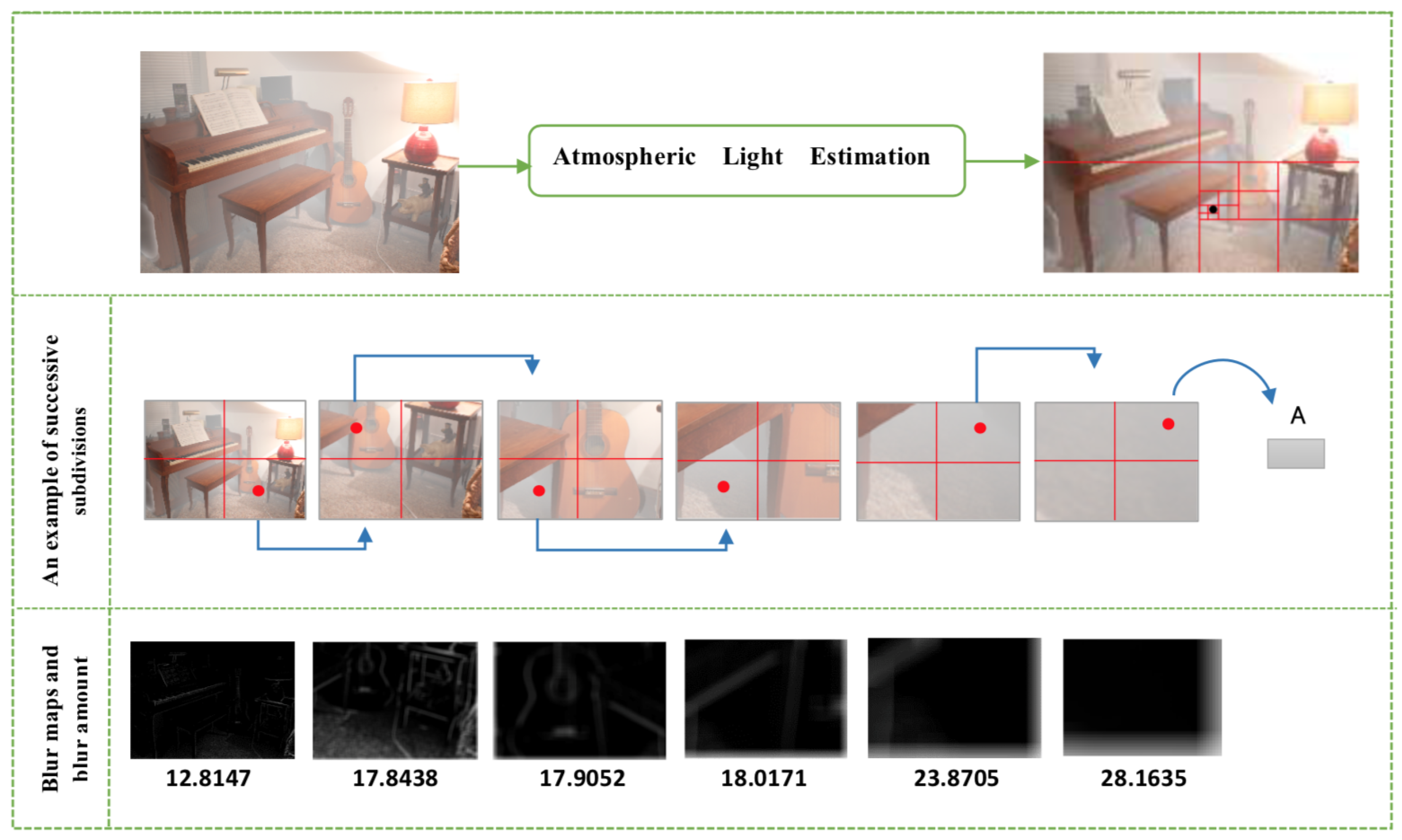
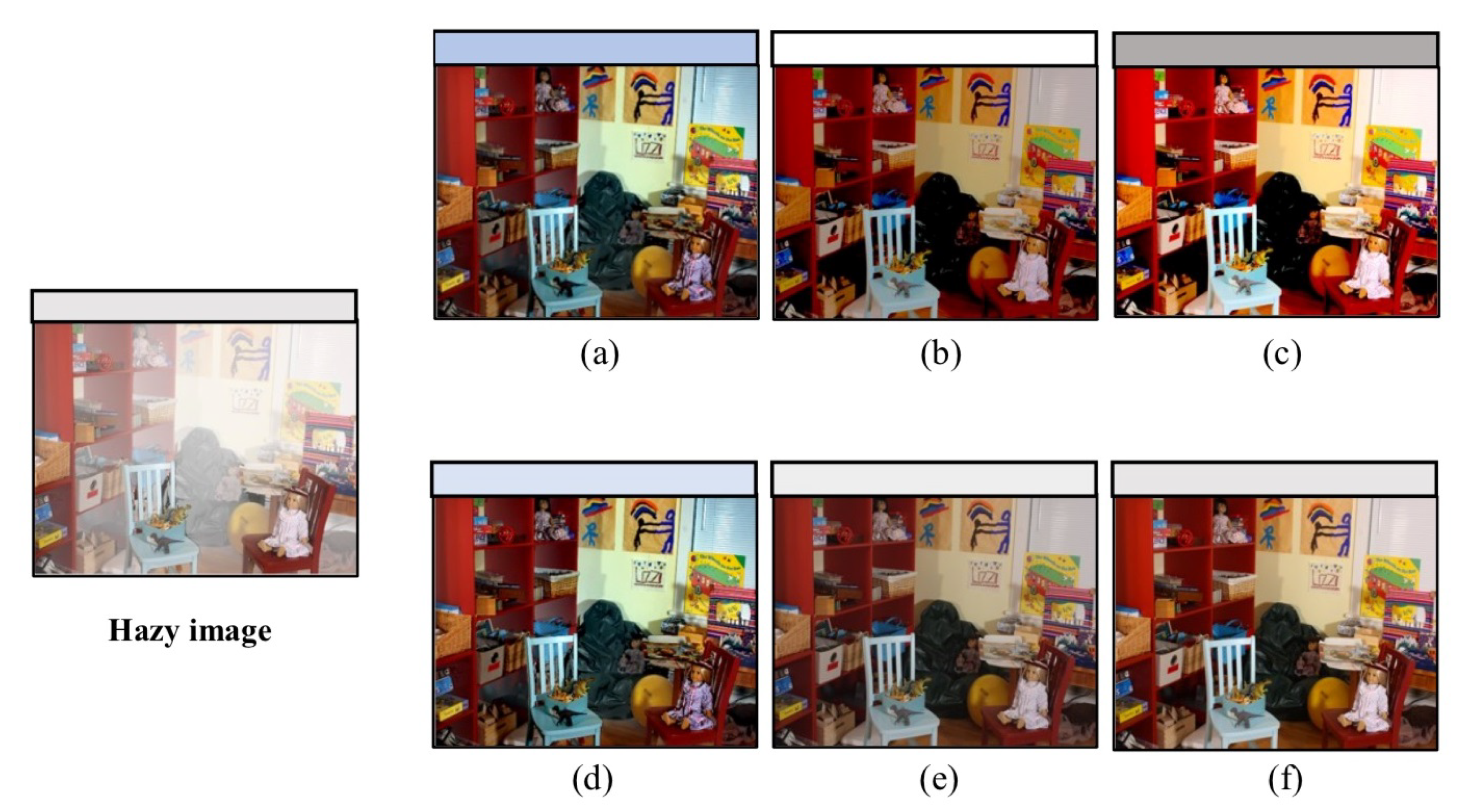
3.1. Atmospheric Light Estimation
| Algorithm 1 A-Est |
|
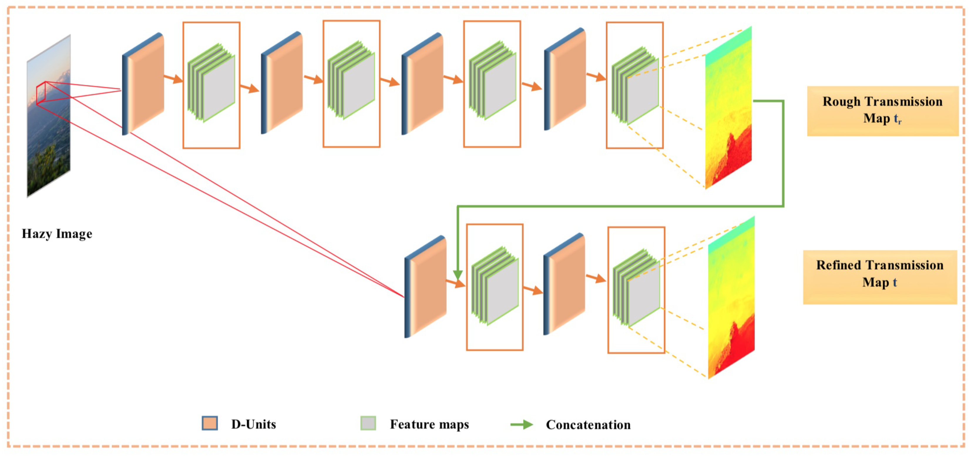
3.2. Transmission Medium Estimation Based on Cascaded Multi-scale CNN
3.2.1. Rough Transmission Map Subnetwork CMCNN
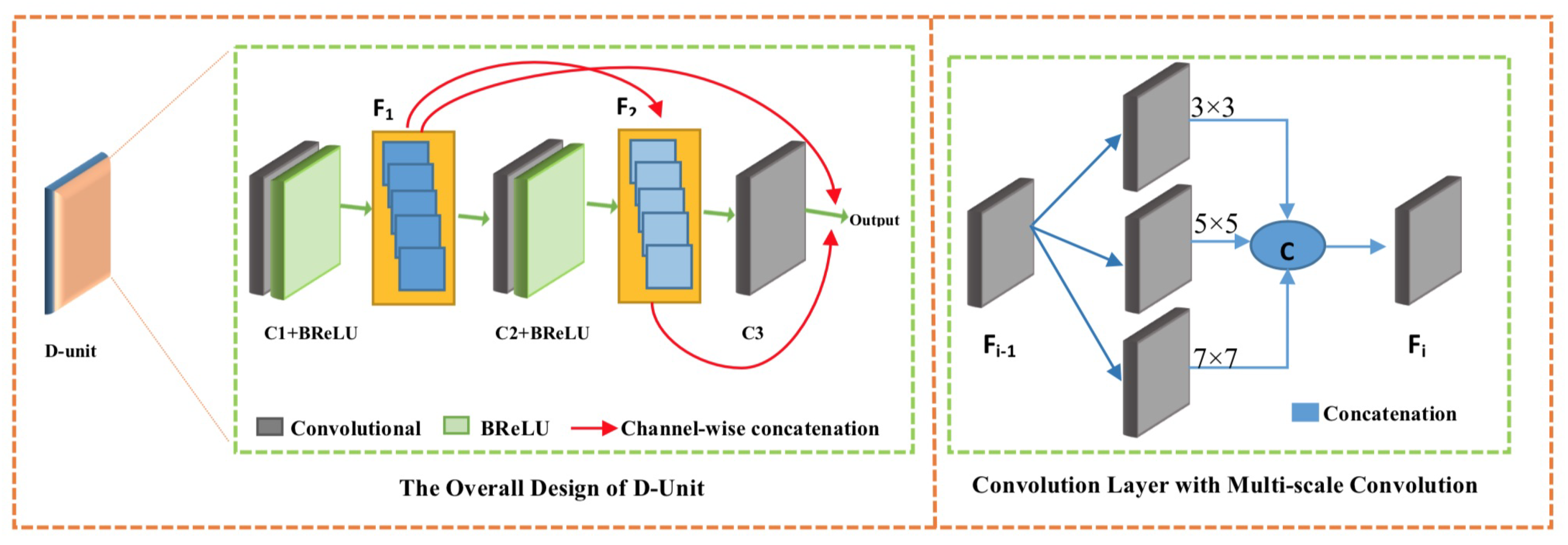
- D-Unit Structure: The overall design of a D-unit is shown in Figure 8 (Left) and comprises three multi-scale convolutional layers pursued by a Bilateral Rectified Linear Unit (BReLU) [28], except for the last convolutional layer. Each convolutional layer represents a fusion of convolutions with a different kernel size (, , and ), thus it is called multi-scale convolution. Regarding the number of filters , for the first and second layers and , we use 16 filters, and for the last layer we use eight filters.The idea of these D-units is inspired by the DenseNet [39] architecture, where layers of each D-unit are densely connected. The output feature maps of each layer are concatenated with those of all succeeding layers; feature maps of the first layer are concatenated with that of the second and third layers and . Moreover, the same for feature maps of are concatenated with feature maps.The proposed D-units-based architecture has significant benefits, e.g. it can avoid the gradient vanishing problem that deep CNNs have with fewer required parameters. In addition, it can maximize the information flow with non-redundancy of feature maps.
- Multi-scale CNN: It is a general truth that human visual perception is a multi-scale neural system. In contrast, using CNN models to solve low-level computer vision tasks always requires the best choice of kernel size. The small size of the filter window can highlight only low-frequency features and neglect the high-frequency content or other important information. Likewise, big kernels can extract only high-frequency details and disregard low-frequency image information. Besides, employing CNNs with successive single filter sizes produces a deeper CNN architecture, which makes the computations complicated and thus hinders the speed of the training process. Therefore, the success of multi-scale CNN representation [26,28] motivates us to apply multi-scale CNN layers in our work to obtain both low- and high-frequency details. In this work, each convolutional layer can be defined as a concatenation of three convolutions with different filter sizes (, , and ), as shown in Figure 8 (right), and can be expressed as:where represents the i-th layer generated feature maps, n is the layer depth (n = 3), and are the output feature maps attained by the three convolutions (, , and ) in each multi-scale CNN layer.
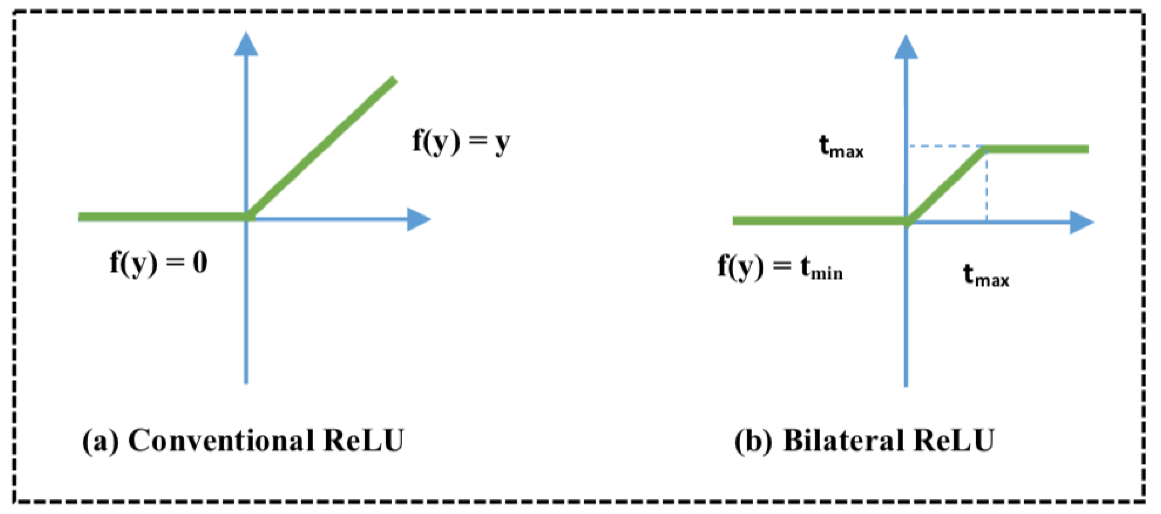
- BReLU: Recently, most of the deep learning methods [26,40] have employed the ReLU as a nonlinear transfer function to solve the problem of vanishing gradient instead of the previous weak sigmoid function [41] that makes the learning convergence very slow. However, the ReLU function [42] is especially designed for classification problems. In this work, we adopt the BReLU function: Cai [28] proposed a sparse representation, benefiting from local linearity of ReLU and preserving the bilateral control of Sigmoid function and considering the restoration problem. Figure 9 shows the difference between the conventional ReLU and Bilateral ReLU; note that =0 and .
- Concatenation: After generating the rough transmission map through CMCNN subnetwork, it is transferred to CMCNN subnetwork as support information, where it is merged with the feature maps extracted by the first unit to explore new features. Exploring new features by using concatenation augments the performance of the CMCNN to predict efficient refined transmission maps.
3.2.2. Refined Transmission Map via CMCNN Subnetwork
3.2.3. Training of CMT
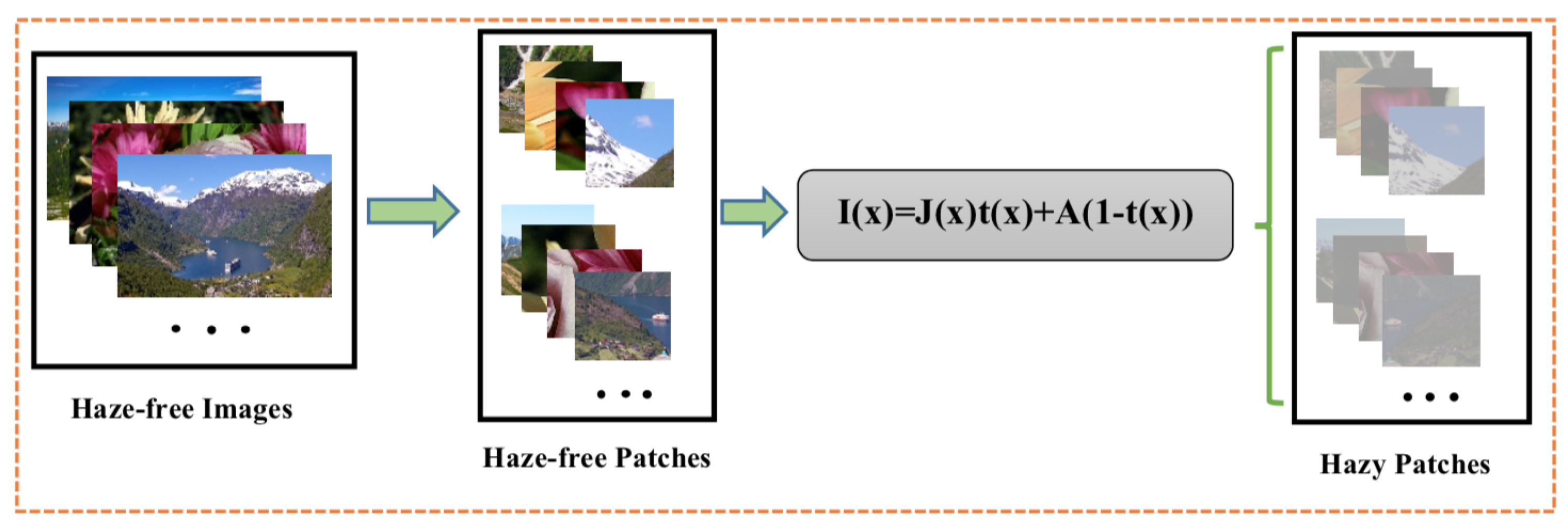
- Training Data: A well-performed network cannot be attained only by making a network with good structure and perfect implementation, but it is also based on the training process. Generally, deep learning networks are data-hungry models. However, it is not easy to provide massive data to train the network, especially for providing pairs of real-world hazy images and their truth transmission maps. Based on the assumption that indicates that the transmission map of an image is constant in small patches, and employing the hazy image formation model (Equation (1), by regarding A = 1), we synthesized a massive number of hazy/clear pairs of patches (as shown in Figure 10). First, we collected from the Internet more than 1000 natural clear images for different scenes (mountain, herb, water, clouds, and traffic). Then, we randomly picked 10 patches of from each image, thus totally we had 10,000 training patches.To reduce the overfitting and make the training process more robust, We added a GaussianNoise layer as the input layer. The amount of noise must be small. Given that the input values are within the range [0, 1], we added Gaussian noise with a mean of 0.0 and a standard deviation of 0.01, chosen arbitrarily.
- Training Strategy and Network Loss: The prediction of the transmission map requires the mapping link between the color image and its corresponding transmission medium through automatic supervised learning. The optimization of the model is realized by minimizing the loss function between I(x) and its truth transmission, with predicting optimal parameters (weights and biases). First, the network feeds on the training image patches I(x) and updates the parameters iteratively, until the loss function reaches the minimum value. The loss function in learning models is a crucial part because it measures the performance of the model to predict the desired result.The extensively used loss function in image dehazing is MSE (Mean Squared Error) that can be expressed as follows:where represents the predicted transmission medium, is the truth transmission medium, and M is the number of hazy image patches in the training data.As noticed, although the loss can maintain both edges and details well during the reconstruction process, it cannot preserve sufficiently the background texture. Therefore, we also consider the SSIM loss [43] in this work to assess the texture and structure similarity. The structural similarity (SSIM) value of each pixel x can be calculated as follows:Note that and are constants of regularization set as default 0.02 and 0.03. , , and represent the average and standard deviation of the predicted image patch x and ground truth image patch y, respectively. Eventually, the loss is calculated as:For the proposed network CMT, the final loss is defined as the aggregation of and as follows:
4. Experimental Results
4.1. Network Implementation
4.2. Network Parameters
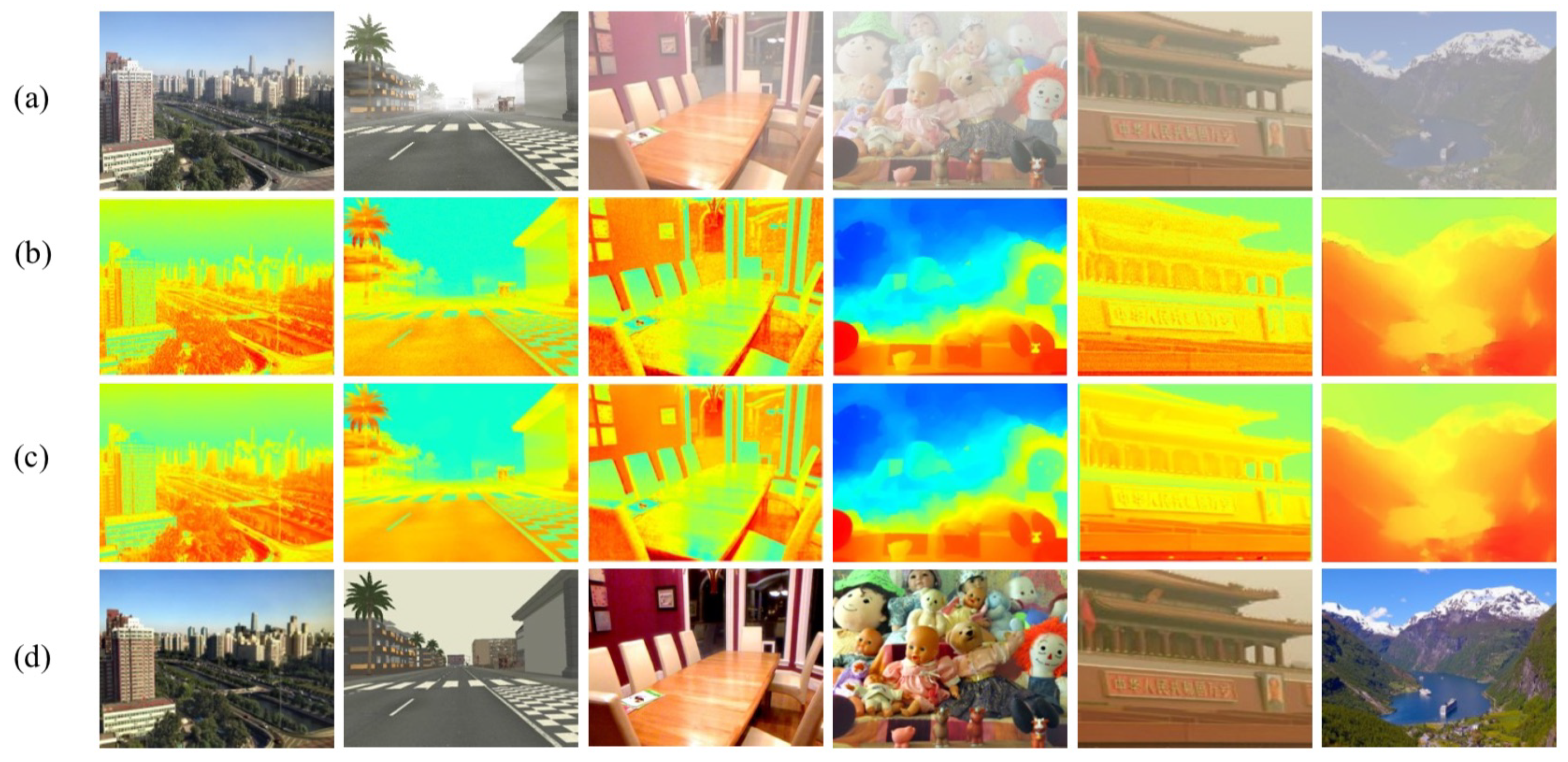
4.3. Haze Removal
4.4. Evaluation of Proposed Method
4.4.1. Qualitative Comparison on Synthetic and Real-world Hazy Images
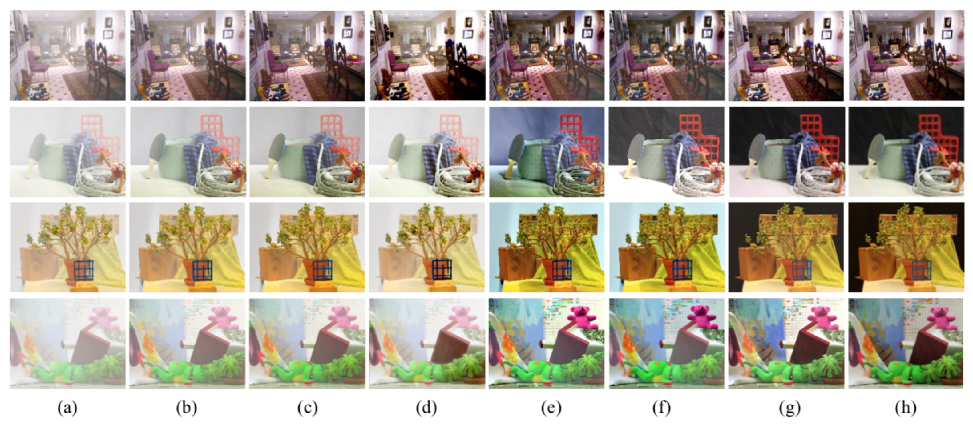
- Comparison on synthetic images: As shown in Figure 13g and Figure 14g, the proposed method has a good performance on hazy synthetic images, where it is not easy to discern our results from the truth images. It achieved good dehazing results, considering haze-removing, color-preserving, visibility-enhancing, and edge-preserving. By contrast, we observe that He et al.’s [14] and Ren et al.’s [26] results still contain a thin haze layer in most synthetic images, especially for thick haze. Thus, these methods are sensitive to the thickness of haze. Cai et al.’s [24] method could lessen haze on images, but it left some haze trace on distant scene objects (e.g., room, teddy, and mountain2 images). On the other hand, Li et al.’s [40] and Salazar-Colores et al.’s [35] methods could remove haze from synthetic images successfully. However, these two methods have a color-shift problem in some regions (e.g., the background of cable image and sky color in park image).
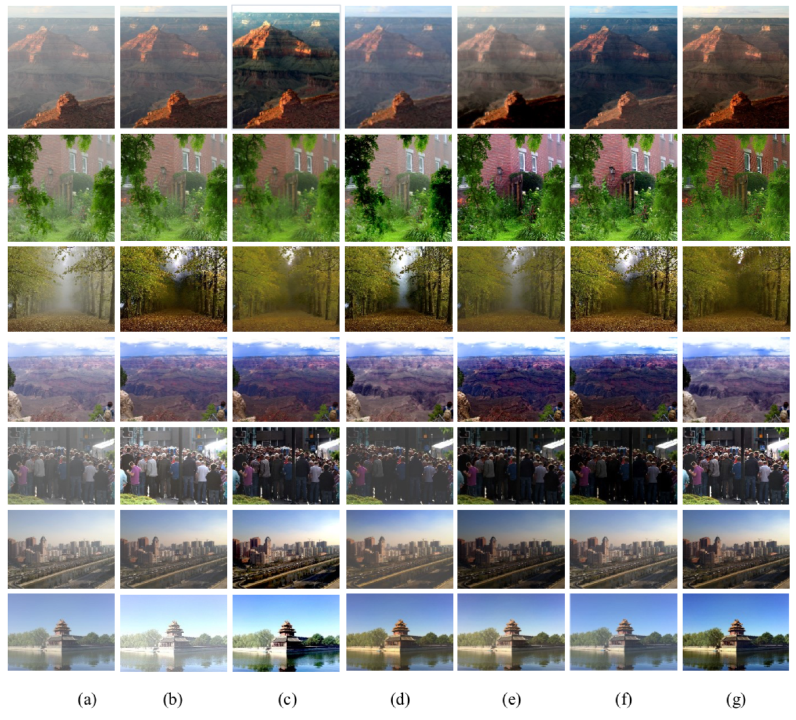
- Comparison on real-world images: In this part, we performed comparisons on the real-world hazy images. The real-world hazy images were collected from the Internet because of the unavailability of a hazy images dataset. Figure 15 demonstrates examples of comparisons on real-world images with comparative methods [14,26,28,35,40].At first glance, we can say that most methods removed haze from images effectively. However, if inspecting carefully, we can discover that He et al.’s [14] method still has some residual haze in specific regions (e.g., tree and forest images). Although the other comparative methods [26,28,35,40] could eliminate haze particles from images efficiently, the over-enhancement problem invades most of the results (e.g., forest, mountain1, and tree images); in addition, these methods generate artificial colors on sky region (mountain1 image). Besides, Cai et al.’s [28] and Li et al.’s [40] results contain halo artifacts caused by edge-deformation. By contrast, our proposed method yielded promising results on real-world images, where it could eliminate haze, produce real vivid colors, and preserve edges of recovered images.
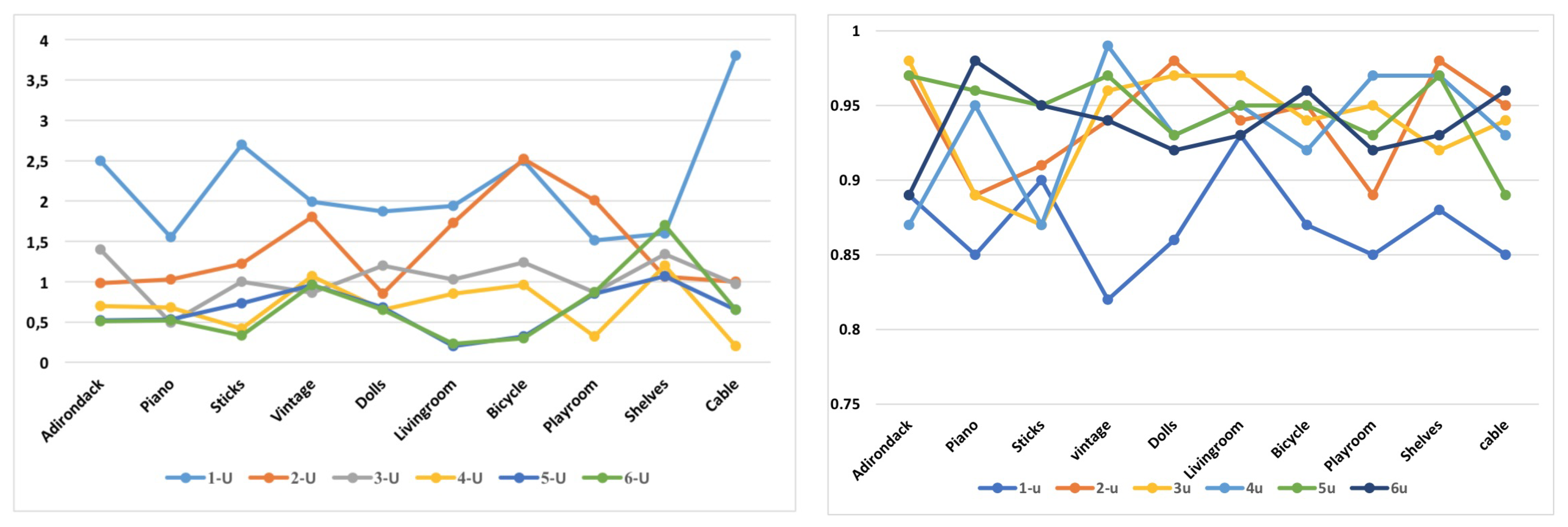
4.4.2. Quantitative Comparison Analysis
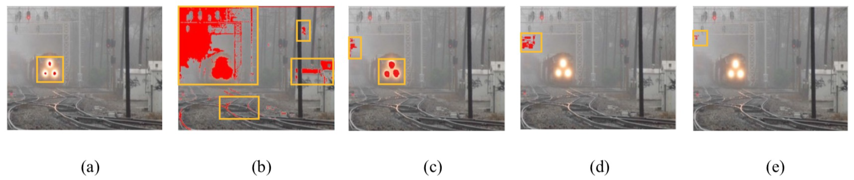
4.4.3. Visual Results on Nighttime Hazy Images
5. Discussion
6. Conclusions
Author Contributions
Funding
Conflicts of Interest
Abbreviations
| MCNN | Multi-scale Convolutional Neural Network |
| CMCNN | Cascaded Multi-scale Convolutional Neural Network |
| BReLu | Bilateral Rectified Linear Unit |
| CMT | Cascaded Multi-scale Network for Transmission map Estimation |
| MRF | Markov Random Field |
| ICA | Independent Component Analysis |
| DCP | Dark Channel Prior |
| CNN | Convolutional Neural Network |
| DNN | Deep Neural Network |
| FR-IQA | Full Reference Image Quality Assessment |
| NR-IQA | No Reference Image Quality Assessment |
References
- Zeng, L.; Yan, B.; Wang, W. Contrast Enhancement Method Based on Gray and Its Distance Double-Weighting Histogram Equalization for 3D CT Images of PCBs. Math. Probl. Eng. 2016, 2016, 1529782. [Google Scholar] [CrossRef]
- Chin, Y.W.; Shilong, L.; San, C.L. Image contrast enhancement using histogram equalization with maximum intensity coverage. J. Mod. Opt. 2016, 63. [Google Scholar] [CrossRef]
- Zhou, L.; Bi, D.Y.; He, L.Y. Variational Histogram Equalization for Single Color Image Defogging. Math. Probl. Eng. 2016. [Google Scholar] [CrossRef]
- Dong, H.; Li, D.; Wang, X. Automatic Restoration Method Based on a Single Foggy Image. J. Image Graph. 2012. [Google Scholar] [CrossRef]
- Zhou, J.; Zhou, F. Single image dehazing motivated by Retinex theory. In Proceedings of the 2nd International Symposium on Instrumentation and Measurement, Sensor Network and Automation (IMSNA), Toronto, ON, Canada, 23–24 December 2013; pp. 243–247. [Google Scholar] [CrossRef]
- Fang, S.; Xia, X.; Huo, X.; Chen, C. Image dehazing using polarization effects of objects and airlight. Opt. Soc. Am. 2014. [Google Scholar] [CrossRef] [PubMed]
- Schechner, Y.Y.; Narasimhan, S.G.; Nayar, S.K. Polarization-Based Vision through Haze. Appl. Opt. 2003, 42, 511–525. [Google Scholar] [CrossRef]
- Schechner, Y.Y.; Narasimhan, S.G.; Nayar, S.K. Blind Haze Separation. In Proceedings of the IEEE Computer Society Conference on Computer Vision and Pattern Recognition CVPR, New York, NY, USA, 17–22 June 2006. [Google Scholar]
- Narasimhan, S.G.; Nayar, S.K. Chromatic Framework for Vision in Bad Weather. In Proceedings of the IEEE Conference on Computer Vision and Pattern Recognition CVPR, Hilton Head Island, SC, USA, 15 June 2000. [Google Scholar]
- Narasimhan, S.G.; Nayar, S.K. Contrast Restoration of Weather Degraded Images. IEEE Trans. Pattern Anal. Mach. Intell. 2003, 25, 713–724. [Google Scholar] [CrossRef]
- Nayar, S.K.; Narasimhan, S.G. Vision in Bad Weather. In Proceedings of the IIEEE International Conference on Computer Vision, Kerkyra, Greece, 20–27 September 1999. [Google Scholar]
- Tan, R.T. Visibility in Bad Weather from a Single Image. In Proceedings of the IEEE International Conference on Computer Vision and Pattern Recognition, Anchorage, AK, USA, 23–28 June 2008. [Google Scholar]
- Fattal, R. Single Image Dehazing. In Proceedings of the ACM SIGGRAPH, Los Angeles, CA, USA, 11–15 August 2008. [Google Scholar]
- He, K.; Sun, J.; Tang, X. Single Image Haze Removal Using Dark Channel Prior. IEEE Trans. Pattern Anal. Mach. Intell. 2011, 33, 2341–2353. [Google Scholar]
- Lin, Z.; Wang, X. Dehazing for Image and Video Using Guided Filter. Appl. Sci. 2012, 2, 123–127. [Google Scholar] [CrossRef]
- Xu, H.; Guo, J.; Liu, Q.; Ye, L. Fast Image Dehazing Using Improved Dark Channel Prior. In Proceedings of the IEEE International Conference on Information Science and Technology, Hubei, China, 23–25 March 2012; pp. 663–667. [Google Scholar] [CrossRef]
- Song, Y.; Luo, H.; Hui, B.; Chang, Z. An Improved Image Dehazing and Enhancing Method Using Dark Channel Prior. In Proceedings of the 27th Chinese Control and Decision Conference, Qingdao, China, 23–25 May 2015; pp. 5840–5845. [Google Scholar] [CrossRef]
- Yuan, X.; Ju, M.; Gu, Z.; Wang, S. An Effective and Robust Single Image Dehazing Method Using the Dark Channel Prior. Information 2017, 8, 57. [Google Scholar] [CrossRef]
- Hsieh, C.; Zhao, Q.; Cheng, W. Single Image Haze Removal Using Weak Dark Channel Prior. In Proceedings of the 9th International Conference on Awareness Science and Technology (iCAST), Fukuoka, Japan, 19–21 September 2018; pp. 214–219. [Google Scholar] [CrossRef]
- Zhu, Q.S.; Mai, J.M.; Shao, L.A. Fast Single Image Haze Removal Algorithm Using Color Attenuation Prior. IEEE Trans. Image Process. 2015, 24, 3522–3533. [Google Scholar] [PubMed]
- Krizhevsky, A.; Sutskever, I.; Hinton, G.E. Imagenet: Classification with Deep Convolutional Neural Networks. In Proceedings of the Advances in Neural Information Processing Systems, Lake Tahoe, NV, USA, 3–6 December 2012; pp. 1097–1105. [Google Scholar]
- Long, J.; Shelhamer, E.; Darrell, T. Fully Convolutional Networks for Semantic Segmentation. In Proceedings of the IEEE Conference on Computer Vision and Pattern Recognition, Boston, MA, USA, 7–12 June 2015. [Google Scholar]
- Fu, M.; Wu, W.; Hong, X.; Liu, Q.; Jiang, J.; Ou, Y.; Zhao, Y.; Gong, X. Hierarchical Combinatorial Deep Learning Architecture for Pancreas Segmentation of Medical Computed Tomography Cancer Images. BMC Syst. Biol. 2018, 12, 56. [Google Scholar] [CrossRef]
- Erhan, D.; Szegedy, C.; Toshev, A.; Anguelov, D. Scalable Object Detection Using Deep Neural Networks. In Proceedings of the EEE Conference on Computer Vision and Pattern Recognition, Columbus, OH, USA, 23–28 June 2014; pp. 2155–2162. [Google Scholar]
- Xie, J.; Xu, L.; Chen, E. Image Denoising and Inpainting with Deep Neural Networks. In Proceedings of the Advances in Neural Information Processing Systems, Lake Tahoe, NV, USA, 3–6 December 2012; pp. 341–349. [Google Scholar]
- Ren, W.; Liu, S.; Zhang, H.; Pan, J.; Cao, X.; Yang, M.H. Single Image Dehazing via Multi-scale Convolutional Neural Networks. In Proceedings of the European Conference on Computer Vision, Amsterdam, The Netherlands, 8–16 October 2016. [Google Scholar]
- Rashid, H.; Zafar, N.; Iqbal, M.J.; Dawood, H.; Dawood, H. Single Image Dehazing using CNN. In Proceedings of the International Conference on Identification, Information and Knowledge in the Internet of Things, IIKI 2018, Beijing, China, 19–21 October 2019; Volume 147, pp. 124–130. [Google Scholar]
- Cai, B.; Xu, X.; Jia, K.; Qing, C.; Tao, D. DehazeNet: An End-to-End System for Single Image Haze Removal. IEEE Trans. Image Process. 2016, 25, 5187–5198. [Google Scholar] [CrossRef] [PubMed]
- Song, Y.; Li, J.; Wang, X.; Chen, X. Single Image Dehazing Using Ranking Convolutional Neural Network. IEEE Trans. Multimed. 2018, 20, 1548–1560. [Google Scholar] [CrossRef]
- Li, C.; Guo, J.; Porikli, F.; Guo, C.; Fu, H.; Li, X. DR-Net: Transmission Steered Single Image Dehazing Network with Weakly Supervised Refinement. arXiv 2017, arXiv:1712.00621v1. [Google Scholar]
- Narasimhan, S.G.; Nayar, S.K. Removing Weather Effects from Monochrome Images. In Proceedings of the IEEE Computer Society Conference of Computer Vision Pattern Recognition CVPR, Kauai, HI, USA, 8–14 December 2001. [Google Scholar]
- Narasimhan, S.G.; Nayar, S.K. Vision and the Atmosphere. In Proceedings of the ACM SIGGRAPH ASIA 2008 Courses -SIGGRAPH Asia 08, Bhubaneswar, India, 16–19 December 2008. [Google Scholar]
- Hu, Y.; Wang, K.; Zhao, X.; Wang, H.; Li, Y.S. Underwater Image Restoration Based on Convolutional Neural Network. Proc. Mach. Learn. Res. 2018, 95, 296–311. [Google Scholar]
- Tao, L.; Zhu, C.; Song, J.; Lu, T.; Jia, H.; Xie, X. Low-light image enhancement using CNN and bright channel prior. In Proceedings of the IEEE International Conference on Image Processing (ICIP), Beijing, China, 17–20 September 2017; pp. 3215–3219. [Google Scholar]
- Salazar-Colores, S.; Cabal-Yepez, E.; Ramos-Arreguin, J.M.; Botella, G.; Ledesma-Carrillo, L.M.; Ledesma, S. A Fast Image Dehazing Algorithm Using Morphological Reconstruction. IEEE Trans. Image Process. 2019, 28, 2357–2366. [Google Scholar] [CrossRef]
- Haouassi, S.; Wu, D.; Hamidaoui, M.; Tobji, R. An Efficient Image Haze Removal Algorithm Based on New Accurate Depth and Light Estimation Algorithm. Int. J. Adv. Comput. Sci. Appl. 2019, 10, 64–76. [Google Scholar] [CrossRef]
- Ali, U.; Mahmood, M.T. Analysis of Blur Measure Operators for Single Image Blur Segmentation. Appl. Sci. 2018, 8, 807. [Google Scholar] [CrossRef]
- Sulami, M.; Glatzer, I.; Fattal, R.; Werman, M. Automatic recovery of the atmospheric light in hazy images. In Proceedings of the IEEE International Conference Computer Photography, Santa Clara, CA, USA, 2–4 May 2014; pp. 1–11. [Google Scholar]
- Huang, G.; Liu, Z.; Weinberger, K.Q.; van der Matten, L. Densely connected convolutional networks. In Proceedings of the IEEE International Conference on Computer Vision and Pattern Recognition (CVPR), Honolulu, HI, USA, 21–26 July 2017; pp. 2261–2269. [Google Scholar]
- Li, C.; Guo, J.; Porikli, F.; Fu, H.; Pang, Y. A Cascaded Convolutional Neural Network for Single Image Dehazing. IEEE Access 2018, 6, 24877–24887. [Google Scholar] [CrossRef]
- Hinton, G.E.; Salakhutdinov, R.R. Reducing the Dimensionality of Data with Neural Networks. Science 2006, 313, 504–507. [Google Scholar] [CrossRef] [PubMed]
- Nair, V.; Hinton, G.E. Rectified Linear Units Improve Restricted Boltzmann Machines. In Proceedings of the 27th International Conference on Machine Learning (ICML-10), Haifa, Israel, 21–24 June 2010; pp. 807–814. [Google Scholar]
- Wang, Z.; Bovik, A.; Sheikh, H.; Simoncelli, E. Image Quality Assessment: From error visibility to structural similarity. IEEE Trans. Image Process. 2004, 13, 3888–3901. [Google Scholar] [CrossRef] [PubMed]
- Kingma, D.; Ba, J. Adam: A method for stochastic optimization. In Proceedings of the International Conference on Learning Representations (ICLR 2015), San Diego, CA, USA, 7–9 May 2015; pp. 87–95. [Google Scholar]
- Tarel, J.P.; Hautiere, N.; Cord, A.; Gruyer, D.; Halmaoui, H. Improved Visibility of Road Scene Images under Heterogeneous Fog. In Proceedings of the IEEE Intelligent Vehicles Symposium (IV’10), San Diego, CA, USA, 21–24 June 2010. [Google Scholar]
- Scharstein, D.; Hirschmller, H.; Kitajima, Y.; Krathwohl, G.; Nesic, N.; Wang, X.; Westling, P. High-resolution stereo datasets with subpixel-accurate ground truth. In Proceedings of the German Conference on Pattern Recognition, Münster, Germany, 3–5 September 2014. [Google Scholar]
- Li, B.; Ren, W.; Fu, D.; Tao, D.; Feng, D.; Zeng, W.; Wang, Z. Benchmarking single-image dehazing and beyond. IEEE Trans. Image Process. 2019, 28, 492–505. [Google Scholar] [CrossRef]
- Choi, L.; You, J.; Bovik, A. Referenceless Prediction of Perceptual fog Density and Perceptual Image Defogging. IEEE Trans. Image Process. 2015, 24, 3888–3901. [Google Scholar] [CrossRef]
- Hautiere, A.; Tarel, J.; Aubert, D.; Dumont, E. Blind Contrast Enhancement Assessment by Gradient Ratioing at Visible Edges. Image Anal. Stereol. 2008. [Google Scholar] [CrossRef]


| Zhu 2015 [20] | Cai 2016 [28] | Sulami 2018 [38] | Salazar-Colores 2018 [35] | Haouassi 2019 [36] | Proposed |
|---|---|---|---|---|---|
| Top 0.1% brightest pixels in depth map | Fixed value (A = 1) | Twice PCA on all haze patches | Top 0.1% brightest pixels in | Top 0.1% brightest pixels in most blurry region with min energy | Top 0.1% blurred pixels |
| CMCNN | Nbre-U | 1-U | 2-U | 3-U | 4-U | 5-U | 6-U |
| MSE-Val | 1.96 | 1.42 | 1.06 | 0.62 | 0.61 | 0.61 | |
| CMCNN | Nbre-U | 1-U | 2-U | 3-U | 4-U | 5-U | 6-U |
| SSIM-Val | 0.87 | 0.94 | 0.94 | 0.94 | 0.95 | 0.95 |
| Method | He et al. [14] | Cai et al. [28] | Ren et al. [26] | Li et al. [40] | Salazar-Colores et al. [35] | Ours |
|---|---|---|---|---|---|---|
| SSIM | 0.727 | 0.853 | 0.821 | 0.898 | 0.887 | 0.912 |
| MSE | 2.093 | 2.892 | 0.846 | 1.867 | 0.079 | 0.068 |
| e | 1.896 | 1.452 | 1.237 | 2.190 | 2.830 | 2.792 |
| 2.951 | 2.763 | 2.609 | 3.652 | 4.025 | 3.785 | |
| FADE | 1.957 | 0.862 | 1.487 | 0.353 | 0.320 | 0.167 |
| T(s) | 14.901 | 1.004 | 1.830 | 0.469 | 0.541 | 0.386 |
| Method | He et al. [14] | Cai et al. [28] | Ren et al. [26] | Li et al. [40] | Salazar-Colores et al. [35] | Ours |
|---|---|---|---|---|---|---|
| e | 1.973 | 1.552 | 1.270 | 2.952 | 3.193 | 2.095 |
| 2.813 | 3.001 | 2.287 | 3.077 | 3.982 | 4.190 | |
| FADE | 2.172 | 0.903 | 1.816 | 0.534 | 0.510 | 0.289 |
| T(s) | 16.033 | 1.002 | 2.071 | 0.658 | 0.782 | 0.453 |
© 2020 by the authors. Licensee MDPI, Basel, Switzerland. This article is an open access article distributed under the terms and conditions of the Creative Commons Attribution (CC BY) license (http://creativecommons.org/licenses/by/4.0/).
Share and Cite
Haouassi, S.; Wu, D. Image Dehazing Based on (CMTnet) Cascaded Multi-scale Convolutional Neural Networks and Efficient Light Estimation Algorithm. Appl. Sci. 2020, 10, 1190. https://doi.org/10.3390/app10031190
Haouassi S, Wu D. Image Dehazing Based on (CMTnet) Cascaded Multi-scale Convolutional Neural Networks and Efficient Light Estimation Algorithm. Applied Sciences. 2020; 10(3):1190. https://doi.org/10.3390/app10031190
Chicago/Turabian StyleHaouassi, Samia, and Di Wu. 2020. "Image Dehazing Based on (CMTnet) Cascaded Multi-scale Convolutional Neural Networks and Efficient Light Estimation Algorithm" Applied Sciences 10, no. 3: 1190. https://doi.org/10.3390/app10031190
APA StyleHaouassi, S., & Wu, D. (2020). Image Dehazing Based on (CMTnet) Cascaded Multi-scale Convolutional Neural Networks and Efficient Light Estimation Algorithm. Applied Sciences, 10(3), 1190. https://doi.org/10.3390/app10031190