An Advanced Reversible Data Hiding Algorithm Using Local Similarity, Curved Surface Characteristics, and Edge Characteristics in Images

Abstract

In this paper, we proposed methods to accurately predict pixel values by effectively using local similarity, curved surface characteristics, and edge characteristics present in an image. Furthermore, to hide more confidential data in a cover image using the prediction image composed of precisely predicted pixel values, we proposed an effective data hiding technique that applied the prediction image to the conventional reversible data hiding technique. Precise prediction of pixel values greatly increases the frequency at the peak point in the histogram of the difference sequence generated using the cover and prediction images. This considerably increases the amount of confidential data that can be hidden in the cover image. The proposed reversible data hiding algorithm (ARDHA) can hide up to 24.5% more confidential data than the existing algorithm. Moreover, it is not possible to determine the presence of hidden confidential data in stego-images, as they possess excellent visual quality. The confidential data can be extracted from the stego-image without loss, and the original cover image can be restored from the stego-image without distortion. Therefore, the proposed algorithm can be effectively used in digital image watermarking, military, and medical applications.

1. Introduction

Data hiding is an important technique for embedding confidential data in cover media such as digital images. A stego-image is generated by hiding confidential data in a cover image, and the confidential data are extracted from the stego-image. Imperceptibility is vital in data hiding, to make it impossible for humans to know whether confidential data is hidden in stego-images [1]. To meet this requirement, the quality of the stego-image must be excellent. Most data hiding techniques that aim to improve the stego-image’s image quality cause distortion in the recovered cover image after extracting the confidential data from the stego-image. Thus, the recovered cover image and the original cover image are inconsistent [2]. The reversible data hiding technique, in which the recovered cover image matches the original cover image, is important in digital image watermarking, military, medical, and digital library [3] applications. Various reversible data hiding techniques have been recently proposed [2,3,4,5,6,7,8,9,10,11,12,13,14,15,16,17,18,19,20,21,22,23,24,25,26,27,28,29,30,31,32,33,34,35,36,37,38]. Various techniques have been proposed to hide data using the least significant bit (LSB) of image pixels [4,5,6,7,8,9]. The data hiding techniques using the LSB of a pixel has a disadvantage in that the restored cover image does not match the original cover image because the LSBs are changed. Data hiding based on wavelet analysis, especially multi-resolution analysis (MRA), has been widely used, and one of the problems with data hiding methods is the visibility of the information contained in the available distributed images [10,11,12,13,14,15]. Data hiding techniques using an additional reference matrix are proposed to increase embedding efficiency [16,17,18,19], and those using pixel value ordering (PVO) are also used [20,21,22,23]. Various reversible data hiding techniques have been recently proposed to hide confidential data by shifting the histogram of an image [24,25,26,27,28,29,30,31,32,33,34,35,36,37,38]. In particular, among these techniques, the techniques of [35,36,37,38] are reversible data hiding techniques using a prediction image. In the techniques of [35,36,37,38], a prediction image is generated by predicting pixel values using surface characteristics present in a cover image, and the prediction image is used to embed confidential data in the cover image.

Ni et al. proposed the NSAS technique using the histogram of an image [1]. This technique examines the peak and zero points in the histogram of a cover image, shifts the pixels between the points, and inserts confidential data into the pixels corresponding to the peak point. Therefore, the technique has a weakness; the maximum number of bits that can be embedded is limited to the frequency at the peak point in the histogram of the cover image.

Li et al. proposed the adjacent pixel difference (APD) technique [2] that improved the NSAS technique. It is a reversible data hiding technique that embeds confidential data using the histogram of an adjacent pixel difference sequence. In this technique, an adjacent pixel difference sequence composed of the differences between adjacent pixels in the cover image is generated, and then its histogram is generated. As adjacent pixels are generally similar to each other, many elements in the sequence have values close to zero. Therefore, the frequency at the peak point in the histogram of the sequence becomes very large, and the number of data bits that can be hidden in the cover image is greatly increased. This technique has a weakness; the number of data bits that can be embedded in the cover image is limited to the frequency at the peak point in the histogram of the adjacent pixel difference sequence.

To solve this issue and hide a large amount of confidential data, various reversible data hiding techniques have been proposed that effectively use the local similarity and the surface characteristics in images [35,36,37,38]. They are based on the APD technique and are effective techniques for hiding a large amount of confidential data in cover image at various levels. The APDLS (adjacent pixel difference using spatial locality and surface characteristics) technique [37,38] can hide more confidential data than the technique of [35,36]. It is a reversible data hiding technique that embeds confidential data using the histogram of a difference sequence generated using the cover image and the prediction image composed of predicted pixel values. The pixel values are precisely predicted in two steps to generate the prediction image. In the first step, locations that are expected to have high local similarity are selected using neighboring pixels. In the second step, the surface characteristics of the image are examined at the locations where local similarity is expected to be high, and pixel values are accurately predicted at the locations by reflecting the surface characteristics. If a difference sequence is generated using the differences between the pixel values of the cover and prediction images, the frequency at the peak point in the histogram of the difference sequence is greatly increased. Therefore, APDLS embeds more data bits in a cover image than the technique of [35,36].

We propose an advanced reversible data hiding algorithm (ARDHA) that performs even better than APDLS. In the ARDHA technique, a prediction image is generated after precisely predicting pixel values according to various curved surfaces and various edge characteristics of an image. Therefore, more pixel value prediction is performed than within the APDLS technique, and the pixel values are accurately predicted. The frequency at the peak point in the histogram of the difference sequence generated using the cover and prediction images is further increased, thereby increasing the number of hidden data bits.

This paper is organized as follows: In Section 2, the existing APD technique is described. In Section 3, we describe the ARDHA technique in detail, and we briefly describe the APDLS technique. In Section 4, the experimental results for evaluating the performance of the ARDHA technique are described and analyzed. The conclusions are described in Section 5, followed by discussion in Section 6.

2. Adjacent Pixel Difference (APD)

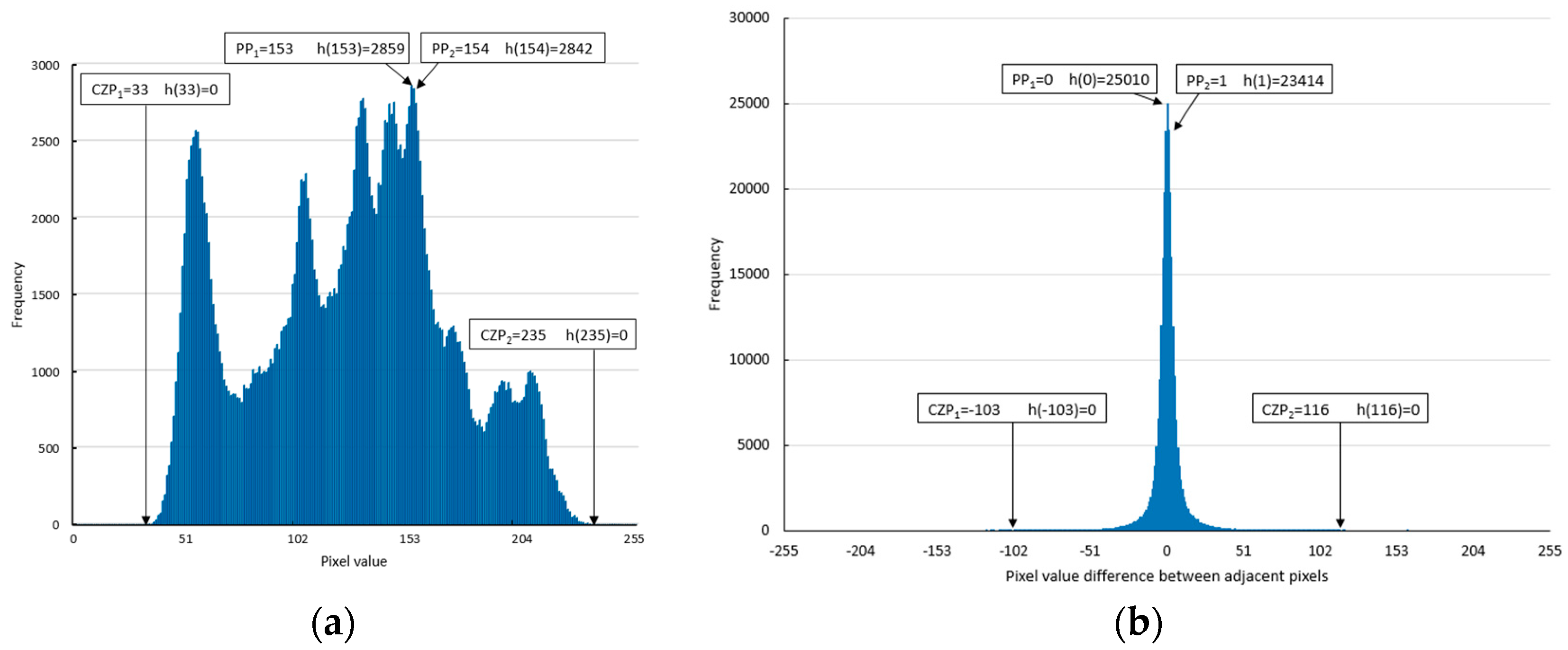
The histogram of Lena, a 512 × 512 gray scale image, is shown in Figure 1a. The pixel values with the highest and second-highest frequencies were PP₁ (peak point 1) and PP₂ (peak point 2), respectively. The pixel values with zero frequencies located closest to the left and right of PP₁ and PP₂ are CZP₁ (closest zero point 1) and CZP₂ (closest zero point 2), respectively. Figure 1a shows that CZP₁ = 33, PP₁ = 153, PP₂ = 154, and CZP₂ = 235.

Ni, Shi, Ansari, and Su proposed the NSAS technique, a reversible data hiding algorithm using a histogram shift [1]. As mentioned previously, the NSAS technique has a weakness; the number of confidential data bits that can be embedded is limited to 5701 bits, which is the sum of h(PP₁) and h(PP₂). The variable h(PP₁) represents the frequency of the pixel value PP₁.

Li et al. proposed the adjacent pixel difference (APD) technique [2] that improved the NSAS technique. The APD technique greatly increases the number of confidential data bits that can be embedded in the cover image by effectively using the property that adjacent pixels have similar values. In the APD technique, the cover image is scanned from left to right and top to bottom in inverse s-order to generate the cover image sequence (C), a sequence of pixel values. Equation (1) is applied to C to generate an adjacent pixel difference sequence (D) consisting of pixel value differences between adjacent pixels. As adjacent pixels are generally similar to each other, many elements of D have values close to zero. Therefore, in the histogram of D, the frequency at zero and values close to zero increases significantly. This is due to the existence of local similarity in images.

$$\begin{gathered} {\mathrm{D}}_{\mathrm{i}}=\{\begin{array}{cc}{\mathrm{C}}_{\mathrm{i}}& \mathrm{if}\mathrm{i}=0\hfill \\ {\mathrm{C}}_{\mathrm{i}-1}-{\mathrm{C}}_{\mathrm{i}}& \mathrm{if}1\le \mathrm{i}\le \mathrm{n}-1\hfill \end{array} \\ \mathrm{where}\mathrm{n}=\left(\mathrm{image}\mathrm{height}\right)·\left(\mathrm{image}\mathrm{width}\right) \end{gathered}$$

(1)

The histogram of D generated by applying Equation (1) to the cover image sequence of Lena is shown in Figure 1b where h(PP₁) is 25,010 bits, and h(PP₂) is 23,414 bits. These values were much larger than those in Figure 1a. In the APD technique, as the histogram of D was shifted to embed confidential data, the maximum number of data bits that could be embedded was h(PP₁) + h(PP₂) = 48,424 bits, which was the sum of the frequencies at peak points PP₁ and PP₂. Therefore, the APD technique could embed 42,723 more bits than the NSAS technique, and the number of confidential data bits that could be embedded was 8.5 times more than the ones embedded in NSAS.

The data embedding procedure of the APD technique is shown in Figure 2. The maximum number of data bits that can be embedded in the cover image is h(PP₁) + h(PP₂), as shown in Step 5 of Figure 2. The symbol (PP_j, CZP_j) used in Equation (2) of Figure 2 represents a set of integers greater than PP_j and less than CZP_j. If PP_j is 1 and CZP_j is 5, then (1, 5) is {2, 3, 4}. The symbol [PP_j +sd_j, CZP_j] used in Equation (7) of Figure 3 represents a set of integers greater than or equal to PP_j +sd_j and less than or equal to CZP_j. If PP_j +sd_j is 1 and CZP_j is 5, then [1,5] is {1, 2, 3, 4, 5}.

The procedure of extracting the confidential data from the stego-image and restoring the original cover image from the stego-image is shown in Figure 3. By following this procedure, the confidential data can be extracted from the stego-image without loss and the original cover image can be restored without distortion. Therefore, the APD technique is an excellent reversible data hiding technique that can embed large amounts of confidential data.

An example of confidential data embedding in APD is shown in Figure 4, and an example of the confidential data extraction and the original cover image restoration procedure is shown in Figure 5. By constructing the histogram of the adjacent pixel difference sequence (D) of the cover image in Figure 4, it can be seen that PP₁ = 0, PP₂ = 1, h(PP₁) = 8, and h(PP₂) = 7. Therefore, the number of data bits that can be embedded in the cover image is h(PP₁) + h(PP₂) = 15 bits. As shown in Figure 4, the stego-image generated by embedding confidential data in the cover image was slightly different from the original cover image, and the image quality of the stego-image was slightly degraded. As shown in Figure 5, the confidential data was extracted from the stego-image without loss, and the original cover image was recovered without distortion. Therefore, the APD technique could be used in digital image watermarking, military, and medical applications.

3. Proposed Algorithm

In general, local similarity, curved surface characteristics, and edge characteristics exist in images. That is, adjacent pixel values of an image are very similar, and various curved surface characteristics such as flat surface, simple inclined surface, simple convex surface, and simple concave surface exist in particular locations of the image. Various edges also exist in specific portions of the image. In the proposed algorithm (ARDHA), the locations where local similarity is expected to be high were selected by using neighboring pixels. Next, it was examined whether a flat surface or a simple inclined surface or a simple convex surface or a simple concave surface exist at each location. At each location where local similarity was not expected to be high, it was examined whether a strong edge or a normal edge or a weak edge exist. Thereafter, the pixel values at each location were accurately predicted according to the investigated characteristics.

A prediction image was generated using the precisely predicted pixel values, and a difference sequence was generated using the cover and prediction images. If the prediction image was generated very close to the cover image, the frequencies at the highest and second-highest peak points in the histogram of the difference sequence increased. Thus, the number of confidential data bits that could be embedded in the cover image could be increased. The more accurate the pixel value prediction, the higher the frequencies at the highest and second-highest peak points in the histogram of the difference sequence, and the greater the number of confidential data bits that could be embedded in the cover image.

The flowchart for obtaining the predicted pixel values to generate the prediction image is shown in Figure 6. Figure 7a shows a sample cover image, and Figure 7b shows the prediction order of the pixel values in a predictable region (the region inside double line marked as Region1. ① to ⑯).

Pixels values are unpredictable in the region outside the double line (two rows on the top and two columns from the left and right sides) as shown in Figure 7b. Figure 7c,d show the neighboring pixels used to predict pixel values at locations ①, ⑤, ⑥, and ⑩ using a flat surface, simple inclined surface, simple convex surface, and simple concave surface characteristics. Figure 7e shows the neighboring pixels used to predict pixel values at locations ⑥ and ⑩ using strong edge, normal edge, and weak edge characteristics. As shown in Figure 7e, at ⑥, 21 pixels in three rows above the location and 3 pixels in the three columns to the right were used to predict the pixel value using the edge characteristics. At ⑩, 21 pixels in three rows above and 3 pixels in the three columns to the left were used to predict the pixel value using the edge characteristics. Therefore, the region where pixel values were predictable using edge characteristics was the remaining portion except three rows on the top and three columns on the left and right sides (the region inside the bold black square marked as Region1(E). ⑥, ⑦, ⑩, ⑪, ⑭, and ⑮). The neighboring pixels used for prediction were the pixels of the cover image that had already been scanned in inverse s-order.

The prediction images generated by applying the APDLS and the proposed ARDHA techniques to the sample image are shown in Figure 7f,g, respectively. As shown in Figure 6, to predict the pixel value, it was necessary to determine whether each location in the inverse s-order was within the region where pixel values were predictable. If the current location is not within Region1, the pixel value of the cover image becomes the predicted pixel value. If the current location is within Region1 where pixel values are predictable, the predicted pixel value is calculated according to the procedure of the proposed technique. As shown in Figure 6, in case of Region1 where pixel values were predictable, the deviation 1 (dev1) obtained using V₁ calculated based on the local similarity was compared with the threshold (β). If dev1 is below β, the surface characteristic at the current location is examined. If any one characteristic of flat, simple inclined, simple convex, and simple concave surfaces exists, the predicted value (V₂ or V_3V or V_3C) is calculated according to the procedure specified to reflect the corresponding surface characteristic.

However, if the current location does not have any of the characteristics of the aforementioned surfaces, V₁ is used as the predicted value. The rounded value of the predicted value (V₁ or V₂ or V_3V or V_3C) is used as the predicted pixel value.

If dev1 is greater than or equal to β, and at the same time, the current location is within Region1(E) and edge characteristic exists at the current location, the predicted value (V_4S or V_4N or V_4W) is calculated according to the procedure specified to reflect the corresponding edge characteristic. The rounded value of the predicted value (V_4S or V_4N or V_4W) is used as the predicted pixel value.

The prediction image was generated using the predicted pixel values. The detailed procedure for predicting pixel values was as follows:

Step 1.1:

If pixel values are predictable at the current location, Step 1.2 is executed. Otherwise, the pixel value of the cover image becomes the predicted pixel value.

Step 1.2:

Based on local similarity, the predicted value V₁, which is calculated using the neighboring pixels and their locational weights, is obtained. At location ①, V₁ is calculated as shown in Equation (9). The coordinates of location ① are (x_i, y_j). The coordinates of pixels with pixel values M, N, O, and R are (x_i+1, y_j−1), (x_i, y_j−1), (x_i−1, y_j−1), and (x_i−1, y_j), respectively. In Equation (9), P(x, y) represents the pixel value at the coordinates (x, y). As shown in Figure 7a, M, N, O, and R are 155, 155, 158, and 160, respectively. As shown in Equation (9), the influence weight of adjacent pixels (M, N, O, and R) on V₁ is set to 1. The influence weight of the remaining pixels (A, B, C, D, E, L, P, and Q) on V₁ is represented by α.

$$\begin{array}{ll}{\mathrm{V}}_1\left({\mathrm{x}}_{\mathrm{i}},{\mathrm{y}}_{\mathrm{j}}\right)& =[\mathrm{P}\left({\mathrm{x}}_{\mathrm{i}+1},{\mathrm{y}}_{\mathrm{j}-1}\right)+\mathrm{P}\left({\mathrm{x}}_{\mathrm{i}},{\mathrm{y}}_{\mathrm{j}-1}\right)+\mathrm{P}\left({\mathrm{x}}_{\mathrm{i}-1},{\mathrm{y}}_{\mathrm{j}-1}\right)+\mathrm{P}\left({\mathrm{x}}_{\mathrm{i}-1},{\mathrm{y}}_{\mathrm{j}}\right)+\{\mathrm{P}\left({\mathrm{x}}_{\mathrm{i}-2},{\mathrm{y}}_{\mathrm{j}-2}\right)\\ & +\mathrm{P}\left({\mathrm{x}}_{\mathrm{i}-1},{\mathrm{y}}_{\mathrm{j}-2}\right)+\mathrm{P}\left({\mathrm{x}}_{\mathrm{i}},{\mathrm{y}}_{\mathrm{j}-2}\right)+\mathrm{P}\left({\mathrm{x}}_{\mathrm{i}+1},{\mathrm{y}}_{\mathrm{j}-2}\right)+\mathrm{P}\left({\mathrm{x}}_{\mathrm{i}+2},{\mathrm{y}}_{\mathrm{j}-2}\right)+\mathrm{P}\left({\mathrm{x}}_{\mathrm{i}+2},{\mathrm{y}}_{\mathrm{j}-1}\right)\\ & +\mathrm{P}\left({\mathrm{x}}_{\mathrm{i}-2},{\mathrm{y}}_{\mathrm{j}-1}\right)+\mathrm{P}\left({\mathrm{x}}_{\mathrm{i}-2},{\mathrm{y}}_{\mathrm{j}}\right)\}·\mathsf{\alpha }]/\left\{4+8·\mathsf{\alpha }\right\}\end{array}$$

(9)

Step 1.3:

To determine the degree of local similarity, the deviation 1 (dev1) between V₁ and the neighboring pixel values is calculated as shown in Equation (10).

$$\begin{array}{ll}\mathrm{dev}1\left({\mathrm{x}}_{\mathrm{i}},{\mathrm{y}}_{\mathrm{j}}\right)& =\mathrm{abs}\left({\mathrm{V}}_1-\mathrm{P}\left({\mathrm{x}}_{\mathrm{i}+1},{\mathrm{y}}_{\mathrm{j}-1}\right)\right)+\mathrm{abs}\left({\mathrm{V}}_1-\mathrm{P}\left({\mathrm{x}}_{\mathrm{i}},{\mathrm{y}}_{\mathrm{j}-1}\right)\right)+\mathrm{abs}\left({\mathrm{V}}_1-\mathrm{P}\left({\mathrm{x}}_{\mathrm{i}-1},{\mathrm{y}}_{\mathrm{j}-1}\right)\right)\\ & +\mathrm{abs}\left({\mathrm{V}}_1-\mathrm{P}\left({\mathrm{x}}_{\mathrm{i}-1},{\mathrm{y}}_{\mathrm{j}}\right)\right)+\{\mathrm{abs}\left({\mathrm{V}}_1-\mathrm{P}\left({\mathrm{x}}_{\mathrm{i}-2},{\mathrm{y}}_{\mathrm{j}-2}\right)\right)+\mathrm{abs}\left({\mathrm{V}}_1-\mathrm{P}\left({\mathrm{x}}_{\mathrm{i}-1},{\mathrm{y}}_{\mathrm{j}-2}\right)\right)\\ & +\mathrm{abs}\left({\mathrm{V}}_1-\mathrm{P}\left({\mathrm{x}}_{\mathrm{i}},{\mathrm{y}}_{\mathrm{j}-2}\right)\right)+\mathrm{abs}\left({\mathrm{V}}_1-\mathrm{P}\left({\mathrm{x}}_{\mathrm{i}+1},{\mathrm{y}}_{\mathrm{j}-2}\right)\right)+\mathrm{abs}\left({\mathrm{V}}_1-\mathrm{P}\left({\mathrm{x}}_{\mathrm{i}+2},{\mathrm{y}}_{\mathrm{j}-2}\right)\right)\\ & +\mathrm{abs}\left({\mathrm{V}}_1-\mathrm{P}\left({\mathrm{x}}_{\mathrm{i}+2},{\mathrm{y}}_{\mathrm{j}-1}\right)\right)+\mathrm{abs}\left({\mathrm{V}}_1-\mathrm{P}\left({\mathrm{x}}_{\mathrm{i}-2},{\mathrm{y}}_{\mathrm{j}-1}\right)\right)+\mathrm{abs}\left({\mathrm{V}}_1-\mathrm{P}\left({\mathrm{x}}_{\mathrm{i}-2},{\mathrm{y}}_{\mathrm{j}}\right)\right)\}·\mathsf{\alpha }\end{array}$$

(10)

Step 1.4:

The obtained dev1 is compared with the threshold (β).

Step 1.5:

If dev1 is less than β, it is determined that the image at the location has a small change in pixel values and a very high local similarity. In this case, Step 1.6 to 1.9 are executed to calculate the predicted value using flat surface, simple inclined surface, simple convex surface, and simple concave surface characteristics. If dev1 is equal to or greater than β, the image at the location is determined as a boundary area with a large change in pixel values. In this case, Step 1.A to 1.E are executed to calculate the predicted value using edge characteristics.

Step 1.6:

The surface characteristic of the image is estimated at that location. The process of estimating the surface characteristic of the image at location ① is as follows: The equation of a straight line passing through any two points (x₁, y₁) and (x₂, y₂) is given by Equation (11). Using Equation (11), the linear equation between adjacent pixels may be determined. Between the pixel having the O value and the adjacent pixel having the N value, a linear equation can be obtained that takes into account only the X-axis direction for the pixel value. That is, the equation E_L(x) of a straight line passing through (x_i−1, O) and (x_i, N) is expressed by Equation (12). In the same way, taking into account only the X-axis direction for the pixel values between N and M, the linear equation E_R(x) is represented by Equation (13). In addition, taking into account only the X-axis direction for the pixel values between R and N, the linear equation E_LD(x) is represented by Equation (14). If all gradients of Equations (12) to (14) are greater than zero, the surface characteristic is estimated as a simple inclined surface where the pixel value on the right is greater than that on the left. If all gradients of Equations (12) to (14) are less than zero, the surface characteristic is estimated as a simple inclined surface whose left pixel value is greater than the right pixel value. If all gradients of Equations (12) to (14) are zero, the surface characteristic is estimated as a flat surface.

If the surface characteristic in the X-axis direction at location ① is a simple inclined surface or a flat surface, the predicted value V₂(x_i, y_j) at location ① is calculated using Equation (15). Thereafter, the rounded value of V₂ is used as the predicted pixel value at location ①. If location ① is not a simple inclined surface or flat surface, Step 1.7 is executed to check the presence of curved surface characteristics at location ①.

$$\mathrm{y}=\{({\mathrm{y}}_2-{\mathrm{y}}_1)/\left({\mathrm{x}}_2-{\mathrm{x}}_1\right)\}\left(\mathrm{x}-{\mathrm{x}}_1\right)+{\mathrm{y}}_1$$

(11)

$${\mathrm{E}}_{\mathrm{L}}\left(\mathrm{x}\right)=\left\{\left(\mathrm{N}-\mathrm{O}\right)/\left({\mathrm{x}}_{\mathrm{i}}-{\mathrm{x}}_{\mathrm{i}-1}\right)\right\}\left(\mathrm{x}-{\mathrm{x}}_{\mathrm{i}-1}\right)+\mathrm{O}$$

(12)

$${\mathrm{E}}_{\mathrm{R}}\left(\mathrm{x}\right)=\left\{\left(\mathrm{M}-\mathrm{N}\right)/\left({\mathrm{x}}_{\mathrm{i}+1}-{\mathrm{x}}_{\mathrm{i}}\right)\right\}\left(\mathrm{x}-{\mathrm{x}}_{\mathrm{i}}\right)+\mathrm{N}$$

(13)

$${\mathrm{E}}_{\mathrm{LD}}\left(\mathrm{x}\right)=\left\{\left(\mathrm{N}-\mathrm{R}\right)/\left({\mathrm{x}}_{\mathrm{i}}-{\mathrm{x}}_{\mathrm{i}-1}\right)\right\}\left(\mathrm{x}-{\mathrm{x}}_{\mathrm{i}-1}\right)+\mathrm{R}$$

(14)

$${\mathrm{V}}_2\left({\mathrm{x}}_{\mathrm{i}},{\mathrm{y}}_{\mathrm{j}}\right)=\left(\mathrm{M}+\mathrm{N}+\mathrm{O}+\mathrm{R}\right)/4$$

(15)

Step 1.7:

The avg(x_i, y_j), which is the average of the neighboring 11 pixels, is calculated using Equation (16). The dev2(x_i, y_j), which is the deviation between avg(x_i, y_j) and the neighboring pixels, is calculated using Equation (17). If dev2(x_i, y_j) is equal to or less than the reference value (ε), Step 1.8 is executed because location ① has a gently changing curved surface characteristic. If dev2(x_i, y_j) is larger than ε, the rounded value of V₁(x_i, y_j) is used as the predicted pixel value.

$$\begin{array}{ll}\mathrm{avg}\left({\mathrm{x}}_{\mathrm{i}},{\mathrm{y}}_{\mathrm{j}}\right)& =\{\mathrm{P}\left({\mathrm{x}}_{\mathrm{i}-2},{\mathrm{y}}_{\mathrm{j}-2}\right)+\mathrm{P}\left({\mathrm{x}}_{\mathrm{i}-1},{\mathrm{y}}_{\mathrm{j}-2}\right)+\mathrm{P}\left({\mathrm{x}}_{\mathrm{i}},{\mathrm{y}}_{\mathrm{j}-2}\right)+\mathrm{P}\left({\mathrm{x}}_{\mathrm{i}+1},{\mathrm{y}}_{\mathrm{j}-2}\right)+\mathrm{P}\left({\mathrm{x}}_{\mathrm{i}+2},{\mathrm{y}}_{\mathrm{j}-2}\right)\\ & +\mathrm{P}\left({\mathrm{x}}_{\mathrm{i}+1},{\mathrm{y}}_{\mathrm{j}-1}\right)+\mathrm{P}\left({\mathrm{x}}_{\mathrm{i}},{\mathrm{y}}_{\mathrm{j}-1}\right)+\mathrm{P}\left({\mathrm{x}}_{\mathrm{i}-1},{\mathrm{y}}_{\mathrm{j}-1}\right)+\mathrm{P}\left({\mathrm{x}}_{\mathrm{i}-2},{\mathrm{y}}_{\mathrm{j}-1}\right)+\mathrm{P}\left({\mathrm{x}}_{\mathrm{i}-2},{\mathrm{y}}_{\mathrm{j}}\right)\\ & +\mathrm{P}\left({\mathrm{x}}_{\mathrm{i}-1},{\mathrm{y}}_{\mathrm{j}}\right)\}/11\end{array}$$

(16)

$$\begin{array}{ll}\mathrm{dev}2\left({\mathrm{x}}_{\mathrm{i}},{\mathrm{y}}_{\mathrm{j}}\right)& =\left|\mathrm{avg}-\mathrm{P}\left({\mathrm{x}}_{\mathrm{i}-2},{\mathrm{y}}_{\mathrm{j}-2}\right)|+|\mathrm{avg}-\mathrm{P}\left({\mathrm{x}}_{\mathrm{i}-1},{\mathrm{y}}_{\mathrm{j}-2}\right)\right|\\ & +\left|\mathrm{avg}-\mathrm{P}\left({\mathrm{x}}_{\mathrm{i}},{\mathrm{y}}_{\mathrm{j}-2}\right)|+|\mathrm{avg}-\mathrm{P}\left({\mathrm{x}}_{\mathrm{i}+1},{\mathrm{y}}_{\mathrm{j}-2}\right)|+|\mathrm{avg}-\mathrm{P}\left({\mathrm{x}}_{\mathrm{i}+2},{\mathrm{y}}_{\mathrm{j}-2}\right)\right|\\ & +\left|\mathrm{avg}-\mathrm{P}\left({\mathrm{x}}_{\mathrm{i}+1},{\mathrm{y}}_{\mathrm{j}-1}\right)|+|\mathrm{avg}-\mathrm{P}\left({\mathrm{x}}_{\mathrm{i}},{\mathrm{y}}_{\mathrm{j}-1}\right)|+|\mathrm{avg}-\mathrm{P}\left({\mathrm{x}}_{\mathrm{i}-1},{\mathrm{y}}_{\mathrm{j}-1}\right)\right|\\ & +\left|\mathrm{avg}-\mathrm{P}\left({\mathrm{x}}_{\mathrm{i}-2},{\mathrm{y}}_{\mathrm{j}-1}\right)\right|+\left|\mathrm{avg}-\mathrm{P}\left({\mathrm{x}}_{\mathrm{i}-2},{\mathrm{y}}_{\mathrm{j}}\right)\right|+\left|\mathrm{avg}-\mathrm{P}\left({\mathrm{x}}_{\mathrm{i}-1},{\mathrm{y}}_{\mathrm{j}}\right)\right|\end{array}$$

(17)

Step 1.8:

If the values of the neighboring pixels satisfy Equations (18) to (21), it is assumed that location ① has simple convex surface characteristic. The predicted value V_3V(x_i, y_j) at location ① is calculated as shown in Equation (26) using Equations (22) to (25). Taking into account only the X-axis direction for the pixel values between Q and R, A and O, and E and M, the linear equations con0[x], con1[x], and con3[x] are represented by Equations (22), (23), and (25), respectively. Similarly, taking into account only the Y-axis direction for the pixel values between C and N, the linear equation is represented by Equation (24). The rounded value of V_3V(x_i, y_j) is used as the predicted pixel value. If all Equations (18) to (21) are not satisfied, Step 1.9 is executed to check the presence of simple concave surface characteristic at location ①

$$\mathrm{P}\left({\mathrm{x}}_{\mathrm{i}-2},{\mathrm{y}}_{\mathrm{j}}\right)<\mathrm{P}\left({\mathrm{x}}_{\mathrm{i}-1},{\mathrm{y}}_{\mathrm{j}}\right)$$

(18)

$$\mathrm{P}\left({\mathrm{x}}_{\mathrm{i}-2},{\mathrm{y}}_{\mathrm{j}-2}\right)<\mathrm{P}\left({\mathrm{x}}_{\mathrm{i}-1},{\mathrm{y}}_{\mathrm{j}-1}\right)$$

(19)

$$\mathrm{P}\left({\mathrm{x}}_{\mathrm{i}},{\mathrm{y}}_{\mathrm{j}-2}\right)<\mathrm{P}\left({\mathrm{x}}_{\mathrm{i}},{\mathrm{y}}_{\mathrm{j}-1}\right)$$

(20)

$$\mathrm{P}\left({\mathrm{x}}_{\mathrm{i}+2},{\mathrm{y}}_{\mathrm{j}-2}\right)<\mathrm{P}\left({\mathrm{x}}_{\mathrm{i}+1},{\mathrm{y}}_{\mathrm{j}-1}\right)$$

(21)

$$\mathrm{con}0\left[\mathrm{x}\right]=\left\{\left(\mathrm{R}-\mathrm{Q}\right)/\left({\mathrm{x}}_{\mathrm{i}-1}-{\mathrm{x}}_{\mathrm{i}-2}\right)\right\}\left(\mathrm{x}-{\mathrm{x}}_{\mathrm{i}-2}\right)+\mathrm{Q}$$

(22)

$$\mathrm{con}1\left[\mathrm{x}\right]=\left\{\left(\mathrm{O}-\mathrm{A}\right)/\left({\mathrm{x}}_{\mathrm{i}-1}-{\mathrm{x}}_{\mathrm{i}-2}\right)\right\}\left(\mathrm{x}-{\mathrm{x}}_{\mathrm{i}-2}\right)+\mathrm{A}$$

(23)

$$\mathrm{con}2\left[\mathrm{y}\right]=\left\{\left(\mathrm{N}-\mathrm{C}\right)/\left({\mathrm{y}}_{\mathrm{i}-1}-{\mathrm{y}}_{\mathrm{i}-2}\right)\right\}\left(\mathrm{y}-{\mathrm{y}}_{\mathrm{i}-2}\right)+\mathrm{C}$$

(24)

$$\mathrm{con}3\left[\mathrm{x}\right]=\left\{\left(\mathrm{M}-\mathrm{E}\right)/\left({\mathrm{x}}_{\mathrm{i}+1}-{\mathrm{x}}_{\mathrm{i}+2}\right)\right\}\left(\mathrm{x}-{\mathrm{x}}_{\mathrm{i}+2}\right)+\mathrm{E}$$

(25)

$$\begin{array}{ll}{\mathrm{V}}_{3\mathrm{X}}\left({\mathrm{x}}_{\mathrm{i}},{\mathrm{y}}_{\mathrm{j}}\right)& =\{\mathrm{K}·\mathrm{avg}\left({\mathrm{x}}_{\mathrm{i}},{\mathrm{y}}_{\mathrm{j}}\right)+\mathrm{con}0\left[{\mathrm{x}}_{\mathrm{i}}\left]+\mathrm{con}1\right[{\mathrm{x}}_{\mathrm{i}}\left]+\mathrm{con}2\right[{\mathrm{y}}_{\mathrm{j}}\right]\\ & +\mathrm{con}3\left[{\mathrm{x}}_{\mathrm{i}}\right]\}/\left\{\mathrm{K}+4\right\}\mathrm{where}\mathrm{x}\in \left\{\mathrm{v},\mathrm{c}\right\}\end{array}$$

(26)

Step 1.9:

If the values of the neighboring pixels satisfy Equations (27) to (30), it is assumed that location ① has simple concave surface characteristic. The predicted value V_3C(x_i, y_j) at location ① is calculated as shown in Equation (26) using Equations (22) to (25). The rounded value of V_3C(x_i, y_j) is used as the predicted pixel value at location ①. If all Equations (27) to (30) are not satisfied, location ① is neither a simple convex surface nor a simple concave surface. Thus, the rounded value of V₁(x_i, y_j) is used as the predicted pixel value at location ①.

$$\mathrm{P}\left({\mathrm{x}}_{\mathrm{i}-2},{\mathrm{y}}_{\mathrm{j}}\right)>\mathrm{P}\left({\mathrm{x}}_{\mathrm{i}-1},{\mathrm{y}}_{\mathrm{j}}\right)$$

(27)

$$\mathrm{P}\left({\mathrm{x}}_{\mathrm{i}-2},{\mathrm{y}}_{\mathrm{j}-2}\right)>\mathrm{P}\left({\mathrm{x}}_{\mathrm{i}-1},{\mathrm{y}}_{\mathrm{j}-1}\right)$$

(28)

$$\mathrm{P}\left({\mathrm{x}}_{\mathrm{i}},{\mathrm{y}}_{\mathrm{j}-2}\right)>\mathrm{P}\left({\mathrm{x}}_{\mathrm{i}},{\mathrm{y}}_{\mathrm{j}-1}\right)$$

(29)

$$\mathrm{P}\left({\mathrm{x}}_{\mathrm{i}+2},{\mathrm{y}}_{\mathrm{j}-2}\right)>\mathrm{P}\left({\mathrm{x}}_{\mathrm{i}+1},{\mathrm{y}}_{\mathrm{j}-1}\right)$$

(30)

Step 1.A:

As the first step of predicting pixel value using edge characteristics, it is determined whether pixel value is predictable at the current location using edge characteristics. If the current location is within Region1(E) (⑥, ⑦, ⑩, ⑪, ⑭, and ⑮), where pixel values can be predicted using the edge characteristics, Step 1.B is executed. If the current location is not within Region1(E), the pixel value of the cover image becomes the predicted pixel value.

Step 1.B:

In this step, four edge values used to predict pixel values are determined. The four edges, which are used to predict pixel value at location ⑥, are shown in Figure 8. To determine the values of the edge(0) to (3), diff[0] to [3] are first calculated according to Equations (31) to (34). Diff[0] to [3] are the sum of the absolute values of the differences between adjacent pixels at 0°, 45°, 90°, and 135° based on the scan direction at the current location. Equations (31) to (34) are expressed based on the coordinates (x_i, y_j) of location ⑥. The values of edge(0) to (3) are calculated using Equation (35). As shown in Equation (35), if the diff value is 0, the corresponding edge is strong and has the value strong_edge. If the diff value is 1, the corresponding edge is normal and has the value normal_edge. If the diff value is 2, the corresponding edge is weak and has the value weak_edge. If the diff value is 3, the corresponding edge is very weak and has the value very_weak_edge. If the diff value is greater than or equal to 4, the corresponding edge has zero value.

$$\mathrm{diff}\left[0\right]=\left|\mathrm{P}\left({\mathrm{x}}_{\mathrm{i}+1},{\mathrm{y}}_{\mathrm{j}}\right)-\mathrm{P}\left({\mathrm{x}}_{\mathrm{i}+2},{\mathrm{y}}_{\mathrm{j}}\right)|+|\mathrm{P}\left({\mathrm{x}}_{\mathrm{i}+2},{\mathrm{y}}_{\mathrm{j}}\right)-\mathrm{P}\left({\mathrm{x}}_{\mathrm{i}+3},{\mathrm{y}}_{\mathrm{j}}\right)\right|$$

(31)

$$\mathrm{diff}\left[1\right]=\left|\mathrm{P}\left({\mathrm{x}}_{\mathrm{i}+1},{\mathrm{y}}_{\mathrm{j}-1}\right)-\mathrm{P}\left({\mathrm{x}}_{\mathrm{i}+2},{\mathrm{y}}_{\mathrm{j}-2}\right)\right|+\left|\mathrm{P}\left({\mathrm{x}}_{\mathrm{i}+2},{\mathrm{y}}_{\mathrm{j}-2}\right)-\mathrm{P}\left({\mathrm{x}}_{\mathrm{i}+3},{\mathrm{y}}_{\mathrm{j}-3}\right)\right|,$$

(32)

$$\mathrm{diff}\left[2\right]=|\mathrm{P}\left({\mathrm{x}}_{\mathrm{i}},{\mathrm{y}}_{\mathrm{j}-1}\right)-\mathrm{P}\left({\mathrm{x}}_{\mathrm{i}},{\mathrm{y}}_{\mathrm{j}-2}\right)|+|\mathrm{P}\left({\mathrm{x}}_{\mathrm{i}},{\mathrm{y}}_{\mathrm{j}-2}\right)-\mathrm{P}({\mathrm{x}}_{\mathrm{i}},{\mathrm{y}}_{\mathrm{j}-3})|$$

(33)

$$\mathrm{diff}\left[3\right]=\left|\mathrm{P}\left({\mathrm{x}}_{\mathrm{i}-1},{\mathrm{y}}_{\mathrm{j}-1}\right)-\mathrm{P}\left({\mathrm{x}}_{\mathrm{i}-2},{\mathrm{y}}_{\mathrm{j}-2}\right)\right|+\left|\mathrm{P}\left({\mathrm{x}}_{\mathrm{i}-2},{\mathrm{y}}_{\mathrm{j}-2}\right)-\mathrm{P}\left({\mathrm{x}}_{\mathrm{i}-3},{\mathrm{y}}_{\mathrm{j}-3}\right)\right|$$

(34)

$$\mathrm{edge}\left(\mathrm{x}\right)=\{\begin{array}{l}\mathrm{strong}\_\mathrm{edge}\mathrm{if}\left(\mathrm{diff}\right[\mathrm{x}]=0)\\ \mathrm{normal}\_\mathrm{edge}& \mathrm{if}\left(\mathrm{diff}\right[\mathrm{x}]=1)\\ \mathrm{weak}\_\mathrm{edge}\mathrm{if}\left(\mathrm{diff}\right[\mathrm{x}]=2)\\ \mathrm{very}\_\mathrm{weak}\_\mathrm{edge}\mathrm{if}\left(\mathrm{diff}\right[\mathrm{x}]=3)\\ 0otherwise\end{array},$$

(35)

$\mathrm{where}\mathrm{x}\in \left\{0,1,2,3\right\}$

Step 1.C:

At location ⑥, if edge(0), or edge(1), or edge(2), or edge(3) has the value strong_edge, the predicted value V_4S(x_i, y_j) is calculated using Equation (36). Thereafter, as shown in Equation (37), if the absolute value of the difference between V₂(x_i, y_j) and V_4S(x_i, y_j) is equal to or less than the difference threshold (δ), the rounded value of V_4S(x_i, y_j) is used as the predicted pixel value. In Equation (37), the value of V₂(x_i, y_j) is (T + U + V + A’)/4. When the absolute value of the difference between V₂(x_i, y_j) and V_4S(x_i, y_j) exceeds δ, the pixel value of the cover image becomes the predicted pixel value. In Equation (37), V(x_i, y_j) represents the predicted pixel value at location (x_i, y_j) and C(x_i, y_j) represents the pixel value of the cover image at location (x_i, y_j).

$$\begin{array}{ll}{\mathrm{V}}_{4\mathrm{S}}\left({\mathrm{x}}_{\mathrm{i}},{\mathrm{y}}_{\mathrm{j}}\right)& =\{{\mathrm{R}}_{\mathrm{s}}·{\mathrm{V}}_2\left({\mathrm{x}}_{\mathrm{i}},{\mathrm{y}}_{\mathrm{j}}\right)+\mathrm{P}\left({\mathrm{x}}_{\mathrm{i}+1},{\mathrm{y}}_{\mathrm{j}}\right)·\mathrm{edge}\left(0\right)+\mathrm{P}\left({\mathrm{x}}_{\mathrm{i}+1},{\mathrm{y}}_{\mathrm{j}-1}\right)·\mathrm{edge}\left(1\right)\\ & +\mathrm{P}\left({\mathrm{x}}_{\mathrm{i}},{\mathrm{y}}_{\mathrm{j}-1}\right)·\mathrm{edge}\left(2\right)+\mathrm{P}\left({\mathrm{x}}_{\mathrm{i}-1},{\mathrm{y}}_{\mathrm{j}-1}\right)·\mathrm{edge}\left(3\right)\}/\{{\mathrm{R}}_{\mathrm{S}}+\mathrm{edge}\left(0\right)\\ & +\mathrm{edge}\left(1\right)+\mathrm{edge}\left(2\right)+\mathrm{edge}\left(3\right)\}\end{array}$$

(36)

$$\mathrm{V}\left({\mathrm{x}}_{\mathrm{i}},{\mathrm{y}}_{\mathrm{j}}\right)=\{\begin{array}{l}{\mathrm{V}}_{4X}\left({\mathrm{x}}_{\mathrm{i}},{\mathrm{y}}_{\mathrm{j}}\right)\mathrm{if}\left(\left|{\mathrm{V}}_2\left({\mathrm{x}}_{\mathrm{i}},{\mathrm{y}}_{\mathrm{j}}\right)-{\mathrm{V}}_{4\mathrm{X}}\left({\mathrm{x}}_{\mathrm{i}},{\mathrm{y}}_{\mathrm{j}}\right)\right|\le \mathsf{\delta }\right)\\ \mathrm{C}\left({\mathrm{x}}_{\mathrm{i}},{\mathrm{y}}_{\mathrm{j}}\right)\mathrm{otherwise}\end{array}$$

(37)

$\mathrm{where}x\in \left\{S,\mathrm{N},\mathrm{W}\right\}$

Step 1.D:

If strong_edge is absent in edge(0), edge(1), edge(2), and edge(3), and at least one of them has normal_edge, then the predicted value V_4N(x_i, y_j) is calculated using Equation (38). The predicted pixel value V(x_i, y_j) is obtained in the same manner as shown in Step 1.C by applying V_4N(x_i, y_j) to Equation (37).

$$\begin{array}{ll}{\mathrm{V}}_{4\mathrm{N}}\left({\mathrm{x}}_{\mathrm{i}},{\mathrm{y}}_{\mathrm{j}}\right)& =\{{\mathrm{R}}_{\mathrm{N}}·{\mathrm{V}}_2\left({\mathrm{x}}_{\mathrm{i}},{\mathrm{y}}_{\mathrm{j}}\right)+\mathrm{P}\left({\mathrm{x}}_{\mathrm{i}+1},{\mathrm{y}}_{\mathrm{j}}\right)·\mathrm{edge}\left(0\right)+\mathrm{P}\left({\mathrm{x}}_{\mathrm{i}+1},{\mathrm{y}}_{\mathrm{j}-1}\right)·\mathrm{edge}\left(1\right)\\ & +\mathrm{P}\left({\mathrm{x}}_{\mathrm{i}},{\mathrm{y}}_{\mathrm{j}-1}\right)·\mathrm{edge}\left(2\right)+\mathrm{P}\left({\mathrm{x}}_{\mathrm{i}-1},{\mathrm{y}}_{\mathrm{j}-1}\right)·\mathrm{edge}\left(3\right)\}/\{{\mathrm{R}}_{\mathrm{N}}+\mathrm{edge}\left(0\right)\\ & +\mathrm{edge}\left(1\right)+\mathrm{edge}\left(2\right)+\mathrm{edge}\left(3\right)\}\end{array}$$

(38)

Step 1.E:

If there is no strong_edge nor normal_edge in edge(0) to (3), and at least one of them has weak_edge, the predicted value V_4W(x_i, y_j) is calculated using Equation (39). The predicted pixel value V(x_i, y_j) is obtained in the same manner as shown in Step 1.C by applying V_4W(x_i, y_j) to Equation (37). If edge(0) to (3) are not strong edges, normal edges, and weak edges, the pixel value of the cover image becomes the predicted pixel value.

$$\begin{array}{ll}{\mathrm{V}}_{4\mathrm{W}}\left({\mathrm{x}}_{\mathrm{i}},{\mathrm{y}}_{\mathrm{j}}\right)& =\{{\mathrm{R}}_{\mathrm{W}}·{\mathrm{V}}_2\left({\mathrm{x}}_{\mathrm{i}},{\mathrm{y}}_{\mathrm{j}}\right)+\mathrm{P}\left({\mathrm{x}}_{\mathrm{i}+1},{\mathrm{y}}_{\mathrm{j}}\right)·\mathrm{edge}\left(0\right)+\mathrm{P}\left({\mathrm{x}}_{\mathrm{i}+1},{\mathrm{y}}_{\mathrm{j}-1}\right)·\mathrm{edge}\left(1\right)\\ & +\mathrm{P}\left({\mathrm{x}}_{\mathrm{i}},{\mathrm{y}}_{\mathrm{j}-1}\right)·\mathrm{edge}\left(2\right)+\mathrm{P}\left({\mathrm{x}}_{\mathrm{i}-1},{\mathrm{y}}_{\mathrm{j}-1}\right)·\mathrm{edge}\left(3\right)\}/\{{\mathrm{R}}_{\mathrm{W}}+\mathrm{edge}\left(0\right)\\ & +\mathrm{edge}\left(1\right)+\mathrm{edge}\left(2\right)+\mathrm{edge}\left(3\right)\}\end{array}$$

(39)

Using the obtained predicted pixel values, a prediction image is generated as shown in Figure 7g. The display rule used in Figure 7f,g is as follows: The general number displayed in the top row represents the pixel value of the cover image. The italic number indicates the rounded value of V₁. The underlined italic number indicates the rounded value of V₂. The italic bold number indicates the rounded value of V_3V. The underlined italic bold number indicates the rounded value of V_3C. The bold number indicates the rounded value of V_4S. The underlined bold number indicates the rounded value of V_4N, and the double underlined bold number indicates the rounded value of V_4W.

The confidential data embedding procedure of the proposed technique is shown in Figure 9, and the procedure for extracting confidential data from the stego-image and restoring the original cover image from the stego-image is shown in Figure 10.

An example of embedding confidential data using the ARDHA technique is shown in Figure 11. An example of extracting the confidential data and restoring the original cover image using the ARDHA technique is shown in Figure 12. The values of the variables used in the examples shown in Figure 11 and Figure 12 are as follows: The alpha (α) used in Equations (9) to (10) was 0.45, the threshold (β) used in Step 1.4 to 1.5 was 10, the reference value (ε) used in Step 1.7 was 10.0, and the K used in Equation (26) was 4.0. The strong_edge, normal_edge, weak_edge, and very_weak_edge used in Equation (35) were 1.00, 0.75, 0.50, and 0.25, respectively. The difference threshold (δ) used in Equation (37) was 1.6. The R_S, R_N, and R_W used in Equations (36), (38), and (39) were 1.1, 0.9, and 0.7, respectively. The reasons for assigning specific values to the variables were explained in the next section.

The predicted values V₁ obtained from Equation (9) at locations ① to ⑯ in Figure 7b were 157.00, 156.30, 155.99, 156.40, 158.11, 156.87, 156.62, 157.29, 157.25, 156.26, 156.88, 158.37, 160.84, 158.75, 156.93, and 155.84. If V₁ is applied to Equation (10), dev1 can be calculated at each location. The dev1 calculated at each location ① to ⑯ were 13.40, 9.54, 6.62, 10.19, 19.89, 11.30, 9.96, 9.66, 15.30, 17.32, 12.21, 17.23, 25.15, 21.60, 20.12, and 18.99, correspondingly. If the surface characteristics of the image are examined at locations ②, ③, ⑦, and ⑧, where dev1 is less than β, the locations with simple inclined surface characteristic or flat surface characteristic in Step 1.5 to 1.6 are ⑦ and ⑧. Therefore, if the predicted V₂ values are obtained at locations ⑦ and ⑧ using Equation (15), they are going to be 158.00 and 156.50, respectively. The values 158 and 157, which are rounded values of V₂, were used as the predicted pixel values at locations ⑦ and ⑧. In Figure 7g, the rounded value of V₂ was indicated by an underlined italic number.

Although dev1 was less than β, the locations without a simple inclined surface or flat surface characteristics were ② and ③. The dev2 values obtained at locations ② and ③ using Equation (17) were 14.55 and 10.00, respectively. Therefore, as shown in Step 1.7, the rounded value of V₁ was used as the predicted pixel value at location ② where dev2 was larger than ε. Therefore, the predicted pixel value at location ② was 156. In Figure 7g, the rounded value of V₁ was indicated by an italic number. At location ③, dev1 was less than β, dev2 was less than or equal to ε, and Equations (27) to (30) were satisfied. Therefore, as shown in Step 1.9, location ③ was determined to have simple concave surface characteristic. Therefore, the predicted value V_3C calculated according to Equations (22) to (26) was 155.38. The value 155, which is rounded value of V_3C, was used as the predicted pixel value at location ③. In Figure 7g, the rounded value of V_3C was indicated by an underlined bold italic number.

At locations ①, ④ to ⑥, and ⑨ to ⑯, where dev1 was greater than or equal to β, the predicted pixel value was obtained as follows: As shown in Step 1.A, locations ①, ④, ⑤, ⑨, ⑫, ⑬, and ⑯ were not within Region1(E). Therefore, the pixel value of the cover image became the predicted pixel value. Locations ⑥, ⑩, ⑪, ⑭, and ⑮ were within Region1(E). Thus, pixel values at these locations could be predicted using edge characteristics. At location ⑥, the values from diff(0) to (3) were 6, 5, 2, and 3. The values from edge(0) to (3) were 0, 0, 0.5 (weak_edge), and 0.25 (very_weak_edge), correspondingly. Therefore, the predicted value V_4W obtained from Step 1.E was 156.2. The rounded value of V_4W was used as the predicted pixel value at location ⑥.

In the same way, the predicted values V_4N, V_4N, V_4S, and V_4N calculated at locations ⑩, ⑪, ⑭, and ⑮ were 156.1, 157.3, 160.0, and 156.5, respectively. The rounded values of V_4N, V_4N, V_4S, and V_4N were used as the predicted pixel values at locations ⑩, ⑪, ⑭, and ⑮, correspondingly. In Figure 7g, the bold number represents the rounded values of V_4S, the underlined bold number represents the rounded values of V_4N, and the double underlined bold number represents the rounded values of V_4W. If we constructed the histogram of the difference sequence (D) in Figure 11, we could see that PP₁ = 0, h(PP₁) = 16, PP₂ = 1, and h(PP₂) = 7. Therefore, the maximum number of data bits that could be embedded in the cover image was 23 bits; 8 bits more than the maximum obtained in APD.

The technique of [35,36] uses only the predicted value V₁, while APDLS [37,38] uses V₂ as well. The techniques [35,36,37,38] were proposed by our research team. The flowchart of pixel value prediction for prediction image generation using the APDLS technique was constructed as follows: In Figure 6, the parts related to V_3V, V_3C, V_4S, V_4N, and V_4W should be removed. If dev1 is greater than or equal to β, the pixel value of the cover image becomes the predicted pixel value. If dev1 is less than β, it is determined whether it is a simple inclined surface or flat surface. If it is a simple inclined surface or flat surface in the X-axis direction, the rounded value of V₂ is used as the predicted pixel value. Otherwise, the rounded value of V₁ is used as the predicted pixel value. By changing Figure 6 as described above, the flow chart of pixel value prediction using APDLS can be obtained.

The prediction image generated by applying the APDLS technique to the sample cover image in Figure 7a is shown in Figure 7f. As shown in Figure 7f, the APDLS technique used only the predicted values V₁ and V₂. The predicted pixel values at locations ② and ③ were 156 and 156, which were the rounded values of V₁. Since locations ⑦ and ⑧ had simple inclined surface characteristics, the predicted pixel values at locations ⑦ and ⑧ were 157 and 158, respectively, which were the rounded values of V₂. Therefore, when the APDLS technique was applied, the prediction image was generated as shown in Figure 7f. After constructing the difference sequence using the cover image and the prediction image, and generating the histogram of the difference sequence, we could see that PP₁ = 0, h (PP₁) = 11, PP₂ = 1, and h (PP₂) = 7. Therefore, the maximum number of data bits that could be embedded in the cover image using the APDLS technique was h(PP₁) + h(PP₂) = 18 bits.

In the APDLS technique, if β is set to 15, and a prediction image is generated for the sample image as shown in Figure 7a, 20 bits can be embedded in the cover image. In the ARDHA technique, if β is set to 15, and a prediction image is generated for the sample image, 24 bits can be embedded in the cover image. If β is set to 20, and the APDLS and the ARDHA techniques are used to generate the prediction image for the sample image, the APDLS and ARDHA techniques can embed 22 and 25 bits in their cover images, respectively. These results occurred because the number of predictions increased as β increased, the frequencies at the highest and second-highest peak points in the histogram of the difference sequence increased, and the number of data bits that could be embedded increased. As the APD technique does not use the prediction image, the embedded bits were always equal to 15 bits, regardless of β.

As shown in Figure 11 and Figure 12, if the ARDHA technique was used to embed confidential data in the cover image, it could embed 8 and 5 more confidential data bits than the APD and APDLS techniques, respectively. In addition, the original confidential data could be extracted without data loss from the stego-image, and the original cover image could be restored without distortion from the stego-image. Therefore, the proposed ARDHA technique could be effectively used in digital watermarking, military, and medical applications.

4. Experimental Results

To evaluate the performance of the proposed ARDHA technique, experiments were carried out using Lena, blackb, Portofino, and ship, which were 512 images × 512 images shown in Figure 13, as cover images. The abstract in this paper was converted to ASCII code and used as confidential data. In the experiments, the confidential data were embedded in the cover image using proposed and existing techniques. The image generated by embedding confidential data in the cover image is called a stego-image.

The values of the variables used in this paper were as follows: the alpha (α) used in Equations (9) to (10) was set to 0.45. In general, local similarity exists in images. Therefore, the closer the pixels are, the more similar the pixel values. To reflect this characteristic, when calculating the predicted value V₁ using Equation (9), the weight of the adjacent pixels affecting the calculation of V₁ was set to 1. The α is the weight that pixels, which are one pixel apart, contribute to the V₁ calculation. To reflect local similarity, we set α to 0.45, which is much smaller than 1.

The experiment was carried out while changing the threshold (β), which is used in Step 1.4 to 1.5, from 0 to 20. The reference value (ε) used in Step 1.7 was set to 10. The dev2 obtained by Equation (17) is the sum of the absolute values of the differences between the avg and the neighboring pixels. If dev2 is much larger than the avg, it is very unlikely that it will be a simple concave surface or a simple convex surface because the change in pixel values around the location is large. For this reason, ε was set to 10; thus, the deviation between the avg and each pixel is less than 1 on average.

The K used in Equation (26) was set to 4. In the cases of simple convex and simple concave surfaces, the pixel values change gently. Therefore, the average value can be used to more accurately predict the pixel values in a simple convex surface or a simple concave surface. K was set to 4 to reflect the avg with the same weight as con0[x_i], con1[x_i], con2[x_i], and con3[x_i].

When predicting pixel values using edge characteristics, strong_edge was set to 1, normal_edge was set to 0.75, weak_edge was set to 0.5, very_weak_edge was set to 0.25, and non-edge was set to 0 in Equation (35). Specific values were set owing to the following reason: The stronger the edge characteristic, the more it should be reflected in the pixel value prediction. Therefore, by setting strong_edge to 1, strong_edge has the greatest influence on the pixel value prediction. By setting no_edge to 0, no_edge has no influence on the pixel value prediction. The normal_edge and weak_edge have values evenly distributed between 1 and 0.

The difference threshold (δ) used in Equation (37) was set to 1.6. To satisfy local similarity, the predicted value V_4X must have a value close to V₂. Therefore, the δ should be set to a small value.

The R_S, R_N, and R_W used in Equations (36), (38), and (39) are 1.1, 0.9, and 0.7, respectively. R_S was determined based on the average of all edge values at all locations with one or more strong edges. R_N was determined based on the average of all edge values at all locations with no strong edges and at least one normal edge. R_W was determined based on the average of all edge values at all locations with no strong or normal edges, and with at least one weak edge.

Lena, blackb, Portofino, and ship images used as cover images are shown in Figure 13a.1–d.1. The stego-images, which are the experimental result images generated by embedding confidential data in cover images using the APD, APDLS, and ARDHA techniques, are shown in Figure 13(a.2–a.11,b.2–b.11,c.2–c.11,d.2–d.11). Figure 13a.2 is a stego-image, which is generated by embedding confidential data into a Lena image using the APD, APDLS(0), and ARDHA-(0) techniques. As explained on the next page, the APD, APDLS(0), and ARDHA-(0) techniques worked the same way. Therefore, as shown in Figure 13a.2, the stego-images generated by embedding confidential data in the cover image using APD, APDLS(0), and ARDHA-(0) techniques are identical. Figure 13(b.2,c.2,d.2) are stego-images generated by embedding confidential data in blackb, Portofino, and ship using the APD, APDLS(0), and ARDHA-(0) techniques. Figure 13a.3–a.6 are stego-images generated by embedding confidential data into a Lena image using APDLS technique, where β is 5, 10, 15, and 20, respectively. Figure 13a.7–a.11 includes stego-images generated by embedding confidential data in Lena image using the ARDHA technique, where β is 0, 5, 10, 15, and 20, respectively. As shown in Figure 13, the visual quality of stego-image generated by applying ARDHA technique is very high. The cover image and the stego-image are visually identical. Thus, it is not possible to visually discern whether confidential data are embedded in the stego-image.

Table 1. Experimental results.

Image	Algorithm	Number of Hidden Bits	PSNR (dB)	Prediction Hit Ratio (%)	Mean of Prediction Errors	Number of Predictions	Increase Rate of Hidden Bits (%)	V1	V2	V3V	V3C	V4S	V4N	V4W
								P.H.R(%) M.P.E N.P	P.H.R(%) M.P.E N.P	P.H.R(%) M.P.E N.P	P.H.R(%) M.P.E N.P	P.H.R(%) M.P.E N.P	P.H.R(%) M.P.E N.P	P.H.R(%) M.P.E N.P
Lena	APD	48424	48.592	-	-	-	-	-	-	-	-	-	-	-
	APDLS(0)	48424	48.592	-	-	-	-	-	-	-	-	-	-	-
	ARDHA-(0)	48424	48.592	-	-	-	-	-	-	-	-	-	-	-
	ARDHA(0)	56256	35.782	17.930	1.94	95362	16.2 (16.2)	-	-	-	-	19.800 1.79 12273	18.159 1.90 37100	17.245 2.02 45989
	APDLS(5)	48485	48.377	31.030	1.12	738	0.1	26.573 1.23 286	33.850 1.05 452	-	-	-	-	-
	ARDHA(5)	56264	35.782	17.947	1.94	95414	16.2 (16.0)	26.882 1.23 279	33.850 1.05 452	60.000 1.00 50	0.000 1.50 2	19.524 1.80 12052	18.050 1.91 36765	17.235 2.02 45859
	APDLS(10)	50451	42.513	21.452	1.55	27801	4.2	20.877 1.57 16870	22.340 1.50 10931	-	-	-	-	-
	ARDHA(10)	56530	35.655	18.016	1.93	100895	16.7 (12.0)	20.897 1.57 16754	22.340 1.50 10931	28.333 1.58 60	23.214 1.63 56	17.921 1.94 8387	16.804 2.04 27338	16.342 2.12 37369
	APDLS(15)	54501	37.847	19.082	1.73	84513	12.5	18.670 1.75 54370	19.825 1.68 30143	-	-	-	-	-
	ARDHA(15)	57773	35.097	17.860	1.91	121879	19.3 (6.0)	18.671 1.75 54254	19.825 1.68 30143	28.333 1.58 60	23.214 1.63 56	16.444 2.16 3825	15.138 2.30 13291	14.770 2.40 20250
	APDLS(20)	56696	35.859	17.902	1.86	122280	17.1	17.497 1.90 78229	18.622 1.79 44051	-	-	-	-	-
	ARDHA(20)	58827	34.453	17.311	1.96	141726	21.5 (3.8)	17.496 1.90 78113	18.622 1.79 44051	28.333 1.58 60	23.214 1.63 56	14.294 2.37 1826	13.642 2.56 6678	13.361 2.65 10942
blackb	APD	57099	48.681	-	-	-	-	-	-	-	-	-	-	-
	APDLS(0)	57099	48.681	-	-	-	-	-	-	-	-	-	-	-
	ARDHA-(0)	57099	48.681	-	-	-	-	-	-	-	-	-	-	-
	ARDHA(0)	71079	35.637	19.153	1.75	121416	24.5 (24.5)	-	-	-	-	20.222 1.64 17333	19.771 1.70 50114	18.236 1.84 53969
	APDLS(5)	57342	48.111	25.132	1.28	1707	0.4	25.680 1.31 662	24.785 1.27 1045	-	-	-	-	-
	ARDHA(5)	71080	35.637	19.150	1.75	121478	24.5 (24.0)	25.426 1.31 645	24.785 1.27 1045	0.000 2.56 9	0.000 1.63 8	20.164 1.64 16872	19.652 1.70 49258	18.191 1.84 53641
	APDLS(10)	66174	39.617	21.759	1.44	67585	15.9	22.309 1.41 45453	20.631 1.51 22132	-	-	-	-	-
	ARDHA(10)	72033	35.426	19.556	1.72	132258	26.2 (8.9)	22.288 1.42 45167	20.631 1.51 22132	16.197 1.77 142	16.667 1.75 144	18.008 1.91 7541	17.988 1.95 24466	16.611 2.06 32666
	APDLS(15)	72885	36.200	20.595	1.55	136578	27.6	21.013 1.52 99044	19.492 1.61 37534	-	-	-	-	-
	ARDHA(15)	73463	34.813	19.628	1.70	155927	28.7 (0.8)	21.000 1.53 98758	19.492 1.61 37534	16.197 1.77 142	16.667 1.75 144	13.653 2.72 1963	13.385 2.76 6739	12.529 2.83 10647
	APDLS(20)	73697	35.225	19.805	1.65	157527	29.1	20.141 1.63 115062	18.893 1.70 42465	-	-	-	-	-
	ARDHA(20)	73828	34.387	19.273	1.75	167744	29.3 (0.2)	20.128 1.63 114776	18.893 1.70 42465	16.197 1.77 142	16.667 1.75 144	11.758 3.32 944	11.856 3.28 3534	10.943 3.38 5739
Portofino	APD	28306	48.650	-	-	-	-	-	-	-	-	-	-	-
	APDLS(0)	28306	48.650	-	-	-	-	-	-	-	-	-	-	-
	ARDHA-(0)	28306	48.650	-	-	-	-	-	-	-	-	-	-	-
	ARDHA(0)	30859	35.438	9.67	3.51	33879	9.0 (9.0)	-	-	-	-	10.341 3.36 2901	9.930 3.47 11329	9.420 3.55 19649
	APDLS(5)	28306	48.644	0.000	3.67	3	0.0	0.000 2.00 2	0.000 7.00 1	-	-	-	-	-
	ARDHA(5)	30859	35.438	9.669	3.51	33880	9.0 (9.0)	0.000 2.00 2	0.000 7.00 1	- - 0	- - 0	10.341 3.36 2901	9.931 3.48 11328	9.421 3.55 19648
	APDLS(10)	28404	47.060	13.685	2.51	1403	0.3	14.712 2.45 904	11.824 2.62 499	-	-	-	-	-
	ARDHA(10)	30893	35.413	9.786	3.49	34417	9.1 (8.8)	14.729 2.45 903	11.824 2.62 499	- - 0	0.000 5.00 1	10.389 3.38 2801	9.848 3.50 10967	9.379 3.57 19246
	APDLS(15)	29494	40.967	11.908	2.69	14881	4.2	11.734 2.69 10721	12.356 2.71 4160	-	-	-	-	-
	ARDHA(15)	31324	34.967	10.071	3.36	41596	10.7 (6.2)	11.735 2.69 10720	12.356 2.71 4160	- - 0	0.000 5.00 1	9.763 3.60 2151	9.238 3.71 8725	8.845 3.76 15839
	APDLS(20)	31539	35.949	11.203	2.93	45621	11.4	11.246 2.91 34625	11.068 2.99 10996	-	-	-	-	-
	ARDHA(20)	32468	33.627	10.375	3.26	62516	14.7 (2.9)	11.247 2.91 34624	11.068 2.99 10996	- - 0	0.000 5.00 1	9.134 4.06 1270	8.336 4.15 5410	7.910 4.13 10215
ship	APD	46430	48.573	-	-	-	-	-	-	-	-	-	-	-
	APDLS(0)	46430	48.573	-	-	-	-	-	-	-	-	-	-	-
	ARDHA-(0)	46430	48.573	-	-	-	-	-	-	-	-	-	-	-
	ARDHA(0)	54880	36.276	19.142	1.84	89578	18.2 (18.2)	-	-	-	-	20.087 1.66 12575	19.800 1.76 36793	18.244 1.96 40210
	APDLS(5)	46549	48.128	22.651	1.39	1192	0.3	19.676 1.41 432	24.342 1.37 760	-	-	-	-	-
	ARDHA(5)	54880	36.273	19.142	1.84	89632	18.2 (17.9)	19.811 1.42 424	24.342 1.37 760	20.000 1.40 5	33.333 1.00 3	19.925 1.67 12286	19.786 1.77 36193	18.210 1.96 39961
	APDLS(10)	51250	41.083	22.043	1.44	47044	10.4	22.023 1.44 30205	22.080 1.44 16839	-	-	-	-	-
	ARDHA(10)	55207	36.103	19.465	1.80	97161	18.9 (7.7)	22.016 1.44 30046	22.080 1.44 16839	21.519 1.56 79	20.000 1.42 80	17.497 1.96 5761	17.669 2.06 19152	16.482 2.25 25204
	APDLS(15)	55212	37.771	20.513	1.58	95664	18.9	20.578 1.58 65250	20.375 1.57 30414	-	-	-	-	-
	ARDHA(15)	56110	35.590	19.254	1.80	113865	20.8 (1.6)	20.571 1.58 65091	20.375 1.57 30414	21.519 1.56 79	20.000 1.42 80	11.923 2.75 1711	13.127 2.88 6437	12.484 3.09 10053
	APDLS(20)	56177	36.396	19.517	1.71	115109	21.0	19.432 1.73 79348	19.706 1.67 35761	-	-	-	-	-
	ARDHA(20)	56529	35.060	18.787	1.86	124825	21.8 (0.6)	19.424 1.73 79189	19.706 1.67 35761	21.519 1.56 79	20.000 1.42 80	9.882 3.29 850	10.723 3.56 3320	9.899 3.78 5546

shows the quantitative values that measured the performance of the proposed technique via experimentation. Table 1 consists of two parts. The performance test results obtained by performing experiments on each of the techniques for calculating the seven predicted pixel values (i.e., V₁, V₂, V_3V V_3C, V_4S, V_4N, and V_4W) used in the ARDHA technique are shown on the right side of the table. The overall performance test results of the ARDHA technique using all seven predicted pixel values are shown on the left side.

The second to eighth columns of Table 1 show the overall results of experiments applying the ARDHA technique to embed confidential data in each cover image. The items of the experimental results from the second to eighth columns in Table 1 are number of hidden bits, PSNR (dB), prediction hit ratio (%), mean of prediction errors, number of predictions, and increase rate of hidden bits (%), respectively. Number of hidden bits represents the number of confidential data bits hidden in the cover image. PSNR (dB) is a measured value that represents the quality of a stego-image. Prediction hit ratio (%) is the number of accurate predictions divided by the total number of predictions, and subsequently multiplied by 100. Mean of the prediction errors represents the sum of the absolute values of the prediction errors divided by the total number of predictions. Number of predictions represents the total number of times the prediction was executed. Increase rate of hidden bits (%) represents the rate of increase in the number of hidden bits expressed as a percentage in the ARDHA and APDLS techniques compared to the APD technique. Compared with the APDLS technique, the increase rate of hidden bits in the ARDHA technique is shown in parentheses.

The last seven columns in Table 1 contain the experimental results of the prediction hit ratio, the mean of prediction errors, and the number of predictions measured when predicting V₁, V₂, V_3V, V_3C, V_4S, V_4N, and V_4W. P.H.R (%) represents the prediction hit ratio, M.P.E represents the mean of the prediction errors, and N. P represents the number of predictions.

In Figure 13 and Table 1, APDLS(v) represent the case where the experiments were carried out by setting β to v in the APDLS technique. ARDHA-(v) represents the ARDHA technique where V_3V, V_3C, V_4S, V_4N, and V_4W are not used and β is set to v. Thus, only V₁, and V₂ are used in ARDHA-(v).

ARDHA(v) indicates the case where β is set to v in the ARDHA technique and uses V₁, V₂, V_3V, V_3C, V_4S, V_4N, and V_4W. ARDHA(0) indicates the case where β is set to 0 in the ARDHA technique. As β is 0, only V_3V, V_3C, V_4S, V_4N, and V_4W are used in ARDHA(0), not V₁ and V₂.

For ARDHA-(0), as β is zero, V₁ and V₂ predictions are not carried out. Therefore, the pixel value of the cover image becomes the pixel value of the prediction image. Thus, the cover image and the prediction image are the same. Thus, as shown in Figure 13 and Table 1, APD and APDLS(0) and ARDHA-(0) worked the same way, and the stego-images generated by applying APD and APDLS(0) and ARDHA-(0) were all the same.

As shown in the last seven columns of Table 1, the larger the β, the greater the number of pixel value predictions obtained using the characteristics of the flat, simple inclined, simple convex, and simple concave surfaces in the image. However, the instances of predicting the pixel values using edge characteristics are reduced. If β is a small value, the number of V_3V and V_3C predictions is greatly reduced. However, as β increases, the number of V_3V and V_3C predictions increases, and the accuracy of pixel value prediction using simple convex surface and simple concave surface characteristics approaches to a high value. These features of the proposed technique can also be easily seen in the flowchart of pixel value prediction in Figure 6. That is, as β increases, on one hand, the case where β is greater than dev1 in Figure 6 increases, and the prediction number for V₁, V₂, V_3V, and V_3C increases. On the other hand, the case where dev1 is greater than or equal to β decreases, and the number of predictions for V_4S, V_4N, and V_4W decreases. Additionally, as β increases, the number of predictions for V_3V and V_3C increases from a small value to a large value, and the prediction hit ratio converges to a constant value.

As shown in the second to eighth columns of Table 1, when predicting pixel values using the ARDHA technique, the number of predictions is very large, the prediction hit ratio is high, and the mean of prediction errors is very small. As the β increases in ARDHA technique, the number of predictions increases. Therefore, a large number of predicted pixel values are used in the prediction image, the prediction image sequence (P) includes a large number of predicted pixel values. Thus, the ARDHA technique increases the frequencies at the highest and second-highest peak points in the histogram of the difference sequence generated by using the cover image and the prediction image. Therefore, the number of confidential data bits that can be embedded in the cover image is increased. For this reason, as indicated in the third and eighth columns of Table 1, as β increases in the ARDHA technique, the number of hidden bits increases, increasing the rate of hidden bits compared to the APD technique.

As shown in Equation (40), when the pixel value prediction is accurate, P_i is the same as C_i. Thus, D_i = C_i–P_i = 0. The more accurate the prediction is, the closer the D_i value is to zero. Therefore, the more accurate the pixel value prediction, the greater the frequencies at the highest and second-highest peak points in the histogram of the difference sequence. Thus, the greater the number of confidential data bits that can be embedded.

When the ARDHA technique was applied, D_i was very small because the mean of prediction errors is very small as shown in Table 1. Thus, the ARDHA technique greatly increases the frequency at the highest and second-highest peak points in the histogram of a difference sequence. Therefore, the number of confidential data bits that can be embedded in the cover image is greatly increased.

The prediction hit ratio in the fifth column of Table 1 was the same as the value calculated using P.H.R and N.P in the last seven columns. The number of predictions in the seventh column of Table 1 was equal to the sum of the N.Ps in the last seven columns. In addition, when the threshold (β) was 5 or more, the total number of prediction times for V₁ and V₂ in the APDLS technique was the same as the total number of prediction times for V₁, V₂, V_3V, and V_3C in the ARDHA technique. These points could be easily seen in the flowchart of pixel value prediction in Figure 6. That is, if β is greater than 0 and dev1 is less than β, the predicted pixel value is determined between V₁, V₂ in the APDLS technique, and the predicted pixel value is determined among V₁, V₂, V_3V, and V_3C in the ARDHA technique. Therefore, the number of predictions for V₁ and V₂ in the APDLS technique was the same as the number of predictions for V₁, V₂, V_3V, and V_3C in the ARDHA technique.

As shown in the fourth column of Table 1, in the ARDHA technique, increasing β from 0 to 20 decreased the PSNR value of the stego-image. However, we could observe in Figure 13 that the visual quality of the stego-image remained very good. Thus, it was not possible to visually discern whether confidential data are embedded in the stego-image. As shown in Figure 13, the cover image and the stego-image were visually identical. As shown in the eighth column of Table 1, when confidential data was embedded in the cover image using the ARDHA technique, the number of hidden bits increased by 29.3% and 24.5% at the maximum compared to the APD and APDLS techniques, respectively.

By applying the proposed technique, it is possible to hide confidential data in the cover image at various levels while maintaining excellent visual quality of the stego-image. The confidential data can be extracted without data loss from the stego-image, and the original cover image can be recovered without distortion from the stego-image. Therefore, the proposed technique can be very useful for digital image watermarking, military, medical applications.

5. Conclusions

In this paper, we proposed the ARDHA technique that can reversibly embed a large amount of confidential data in a cover image at various levels. In the proposed ARDHA technique, a prediction image was generated using seven kinds of predicted pixel values, and the prediction image was used to embed confidential data in the cover image. Due to the high accuracy of the seven kinds of pixel value predictions used in the ARDHA technique, a prediction image closely approximating the cover image was generated. Thus, by embedding confidential data in the cover image using a prediction image closely approximating the cover image, a large amount of confidential data could be embedded at various levels, while maintaining the excellent visual quality of the stego-image.

As the visual quality of a stego-image generated by applying ARDHA technique was very high, it was not possible to distinguish the stego-image from the cover image. Thus, it was not possible to visually discern whether confidential data are embedded in the stego-image. Using the ARDHA technique, the number of confidential data bits that could be embedded in the cover image was increased by 29.3% and 24.5% compared to the APD and APDLS techniques, respectively. In addition, the confidential data could be extracted without data loss from the stego-image and the original cover image could be restored without distortion from the stego-image. Therefore, the proposed ARDHA technique was an efficient reversible data hiding algorithm that is very useful in digital image watermarking, military, and medical applications.

6. Discussion

Compared to the previous research, we proposed an effective reversible data hiding technique that uses various curved surface characteristics and various edge characteristics such as simple convex surface, simple concave surface, strong edge, normal edge, and weak edge to hide large amounts of confidential data in the cover image at various levels. The experiments proved the superiority of the proposed technique. However, unlike the previous researches, the execution time of the proposed technique was increased because the parts that accurately predict pixel values were added using the aforementioned surface characteristics and edge characteristics. Therefore, in the proposed technique, there is a trade-off between the amount of hidden data and the execution time, which requires further research. In addition, the applicability of the proposed technique can be improved by conducting research on hiding confidential data in color images, text data, and voice data based on the proposed technique in this paper.