Article

Integration of Refined Composite Multiscale Cross-Sample Entropy and Backpropagation Neural Networks for Structural Health Monitoring

Department of Civil Engineering, National Chiao Tung University, Hsinchu 30010, Taiwan
*
Author to whom correspondence should be addressed.
Appl. Sci. 2020, 10(3), 839; https://doi.org/10.3390/app10030839
Submission received: 31 October 2019 / Revised: 18 January 2020 / Accepted: 20 January 2020 / Published: 24 January 2020
(This article belongs to the Special Issue Vibration-Based Structural Health Monitoring)

Abstract

:
This study developed a structural health monitoring (SHM) system based on refined composite multiscale cross-sample entropy (RCMCSE) and an artificial neural network for monitoring structures under ambient vibrations. RCMCSE was applied to enhance the reliability of entropy estimations. First, RCMCSE was implemented to extract damage features, and finite element analysis software was then used to generate training samples, which included stiffness reductions to achieve various damage patterns. A neural network model was constructed and trained using entropy values for these damage patterns. An experiment was conducted on a seven-story steel benchmark structure to validate the performance of the proposed system. Additionally, a confusion matrix was established to evaluate the performance of the proposed system. The results obtained for a scaled-down benchmark structure indicated that 89.8% of the floors were accurately classified, and 90% of the practical damaged floors were correctly diagnosed. The performance evaluation demonstrated that the proposed SHM system exhibited increased damage location accuracy.

1. Introduction

Disasters such as earthquakes and typhoons degrade the strength of structures. To protect property and lives, the structural health of buildings must be inspected after such natural disasters. In civil engineering, structural health monitoring (SHM) is applied to detect damage to structures. Novel SHM methods based on signal processing techniques have recently been proposed to analyze measured structural responses. In 2001, Sohn et al. [1] applied a statistical process control technique and a pattern recognition technique to diagnose the vibration-based damage. Lam et al. [2] utilized the model updating approach to set up a damage criterion in 2004. Structural dynamic responses, such as velocity and acceleration, can be collected to determine the structural health condition of a building. SHM results can serve as the basis to implement suitable structural retrofit.
In recent years, entropy has been used in different fields. Multiscale entropy (MSE) approaches have been applied to extract information from biological signals affected by noise. For example, Costa et al. [3,4] have proposed an MSE method and used it to separate healthy individuals from patients with congestive heart failure and patients with erratic cardiac arrhythmia. According to this study, analysis based on a single time scale cannot comprehensively extract heart signal information. This has thus led to the emergence of the concept of multiscale analysis, in which a coarse-grained process is utilized to divide a time signal into several time scales; this thus increases the feasibility and accuracy of entropy measures. In 2013, Wu et al. [5] applied a composite Multiscale entropy (CMSE) method to identify gear damage; white noise and pink noise were used to prove that the CMSE method could reduce the standard deviation (SD) of entropy values. In addition, CMSE was reported to provide more accurate entropy values than MSE. Nevertheless, CMSE application resulted in undefined entropy values. In 2014, S.D. Wu et al. [6] proposed a refined composite Multiscale entropy (RCMSE) approach. The RCMSE approach was demonstrated to increase the accuracy of entropy estimation and reduces the probability of inducing undefined entropy values for analyses of short time series.
Because entropy is a statistical concept, artificial intelligence (AI) technology is used to differentiate entropy values. AI technology, including artificial neural networks (ANNs) and machine learning, has been applied in several fields. In 1992, Wu et al. [7] applied a backpropagation neural network (BPN) to identify damage on a three-story steel structure. In 1993, Elkordy et al. [8] applied a BPN to identify changes in the vibrational signatures of a structure and consequently detect damage. Moreover, in 1994, Kartam et al. [9] demonstrated the versatility of neural networks as a problem-solving tool and determined that such networks can be applied to solve different problems in civil engineering. In 2012, S.D. Wu et al. [10] used permutation entropy (PE) to extract the features of bearing faults; in addition, they incorporated a support vector machine to classify damage cases. In 2013, Tiwari et al. [11] combined multiscale PE and adaptive neuro-fuzzy systems to develop a bearing fault diagnosis system.
The aim of the present study was to quantify entropy values. The flowchart of the study is presented in Figure 1. An ANN-based technique was applied to distinguish between signals obtained from damaged and healthy structures. Finite element model was applied to generate a training database for the ANN. The proposed system was validated by numerical simulation of a seven-story structure under the ambient vibration response and a series of steel structure experiment.
The flowchart of the study procedures is shown in Figure 1. RCMSE is adopted to improve the stability and reliability when evaluating the entropy value of a system. Numerical model is first used to generate the damage database, and the entropy statics are collected. An ANN based on the entropy value is then trained to detect the damage condition and location, and the damage can be automatically classified by the proposed health index. In order to evaluate the performance of the proposed system, an experiment test of a scale-down steel structure is conducted. Through the whole process, the proposed SHM system can be established.

2. Materials and Methods

2.1. Refined Composite Multiscale Cross-Sample Entropy (RCMCSE) Approach

Cross-sample entropy (Cross-SampEn) is typically applied to evaluate the degree of dissimilarity between two time series. However, Cross-SampEn is not applicable to all problems for a more accurate value. Hence, RCMCSE was proposed to solve some problems such as the statistical reliability of Cross-SampEn was reduced as time scale increased [12]. RCMCSE, which is based on Cross-SampEn and MSE, is applicable to more problems compared with Cross-SampEn because of modifications to its calculation procedures. The RCMCSE and Cross-SampEn procedures are summarized as follows.
First, regarding Cross-SampEn, consider two time series with N points: { X i }   =   { x 1 ,   ,   x i ,   ,   x N } and { Y j }   =   { y 1 ,   ,   y j ,   ,   y N } . These time series can be divided into templates of length m.
u m ( i )   =   { x i ,   x i + 1 ,   ,   x i + m - 1 } ,   1     i     N     m   +   1
v m ( j )   =   { y j ,   y j + 1 ,   ,   y j + m - 1 } ,   1     j     N     m   +   1
The number of similarities is n i m ( r ) , and it can be defined as the maximum distance between two templates i and j. The formula of n i m ( r ) is expressed as follows:
n i m ( r )   =   j   =   1 N - m d [ u m ( i ) ,   v m ( j ) ]
d [ u m ( i ) ,   v m ( j ) ]   =   max { | x ( i + k ) y ( j + k ) | :   0     k     m   -   1 }
d [ u m ( i ) ,   v m ( j ) ]     r ,   1     j     N     m
The probability of similarity between the templates is calculated through the following equations
U i m ( r ) ( v | | u )   =   n m ( r ) ( N   -   m )
The average probability of similarity of the templates with the length m is calculated as follows:
U m ( r ) ( v | | u )   =   1 ( N   -   m ) i   =   1 N - m U i m ( r ) ( v | | u )
Next, new templates are created with different template lengths m+1. The average probability of similarity U m + 1 ( r ) ( v | | u ) is the procedure of averaging the probability of similarity. Cross-SampEn is defined as follows:
CS E ( m ,   r ,   N )   =   - ln { U m + 1 ( r ) ( v | | u ) U m ( r ) ( v | | u ) }
Second, RCMCSE comprises more procedures than Cross-SampEn. It includes a coarse-graining procedure that is applied to analyze two time series at a given scale factor. Each point in the coarse-grained time series is defined as follows:
x j ( τ )   =   1 τ i   =   ( j   - 1 ) τ + 1 j τ x i ,   1     j     N τ
y j ( τ )   =   1 τ i   =   ( j   - 1 ) τ + 1 j τ y i ,   1     j     N τ
For MSCE, the length of the time series decreases when the coarse-graining procedure is applied to the original time series. Therefore, using MSCE to analyze a short time series may lead to inaccurate Cross-SampEn results at large time scales. To resolve this problem, CMSE was previously proposed [5]. On the basis of CMSE, CMCSE can be defined as follows:
C M C S E ( x , y , τ , m , r ) = 1 τ k = 1 τ S a m p E n ( x k ( τ ) , y k ( τ ) , m , r )
The CMCSE value is the mean of τ Cross-SampEn values. However, the CMCSE value is undefined if one of the values of n k , τ m or n k , τ m + 1 is zero. Therefore, the RCMCSE method was proposed [6] to address the problem of undefined entropy values. In contrast to CMCSE, RCMCSE involves the assumption that n k , τ m and n k , τ m + 1 represent the means of n k , τ m and n k , τ m + 1 , respectively. Instead of averaging entropy values, RCMCSE averages the sum of the number of similarities.
n ¯ k , τ m = 1 τ k = 1 τ n k , τ m

2.2. Backpropagation Neural Network (BPN) System

A BPN is a neural network system that uses Widrow–Hoff learning rules to conduct generalization. A BPN has multiple layers and applies nonlinear activation functions to identify the relationship between inputs and outputs. Specifically, the network system associates an input with a defined target and classifies the input types. The BPN algorithm involves error backpropagation; the structure of a BPN is illustrated in Figure 2.
A BPN is a feedforward neural network and utilizes the back-propagation learning algorithm. In forward transmission, data are processed from the input layer to the next layer through relevant weights; subsequently, the error is calculated as the difference between the actual output and calculated output. The aim of backpropagation is to revise weights when the error is excessively high. Because a BPN is a supervised learning algorithm, it calculates the difference between the target output and calculated output using an energy function to reduce errors. This correction method is called gradient descent; the energy function is used to revise the weights in the network. In conclusion, backpropagation can be used to minimize error values. The energy function can be expressed as follows:
F ( x ) = E [ e 2 ] = E [ ( t a ) 2 ]
where t is the target output and a is the calculated output.

2.3. Proposed Structural Health Monitoring (SHM) Algorithm

Entropy is a concept of complexity, and manually classifying it is difficult. In this study, an ANN was applied to quantify entropy. The study developed an SHM system based on RCMCSE and a BPN. First, structural responses under ambient vibrations were recorded by sensors that collected velocity data. A numerical model was established to generate different damage cases as the training database for the BPN. Next, RCMCSE was applied to extract damage features, and the BPN was used to express entropy values. Finally, new test data were automatically classified by the system; thus, the structural situation could be clearly identified.

3. Numerical Simulation

3.1. Numerical Model

In this study, the finite element software ETABS (V17, CSI Computers and Structures, Inc, Walnut Creek, CA., USA and 2017) was used to construct a seven-story benchmark structure in numerical simulation [13]. The geometrical properties of this model are outlined as follows:
  • The model was a steel structure with yield strength of F y   of   0.24525   Pa .
  • The height of each story was 1.06 m, and the column cross-sectional area was 0.025   ×   0.15   m 2 .
  • L-shaped steel angles measuring 0.065   ×   0.065   ×   0.006   m 3 were used to brace the structure in the Y-axis.
  • The beam was a steel plate with a cross-sectional area of 0.10   ×   0.07   m 2 .
  • The area of each story was 1.32   ×   0.92   m 2 , and the floor lengths on the x- and y-axes were 1.32 and 0.92 m, respectively. An additional 500 kg was placed on each floor to simulate real structural behavior.
Time history analysis used white noise to simulate ambient vibrations. In ETABS, a white noise of 1 MW power was set as the acceleration input along the y-axis with a wide bandwidth of 100 Hz. The sampling rate was 200 Hz, and the total time was set to 5 min. After the database was created by conducting the time history analysis for each damage cases, velocity response data were extracted from the center of each floor along the y-axis. The ETABS model and damage scenario are presented in Figure 3a,b. The modal frequencies were used as a criterion for modelling, and the details of the modal frequencies are presented in Table 1.

3.2. Database Setup

In this study, an SHM system based on RCMCSE and the BPN was developed and used for damage analysis. RCMCSE was used for damage feature extraction, and the BPN was applied for damage quantification. To reflect the possible damage condition of and location on the structure, the numerical model was simulated to have residual stiffness of 0% (representing a damage case), 35%, 70%, and 100% (representing a healthy case) for each floor. This study defined different damage cases with the removal of bracings. Both bracings on each floor were replaced with different section bracings to simulate stiffness reductions. Accordingly, ETABS was used to create a database of different stiffness reduction cases.
According to previous research [12] discussing detection accuracy under different parameter combinations, RCMCSE parameters such as the template length m, threshold r, and signal length N were optimized as 4, 0.08 × SD of the time series, and 20,000 points, respectively. Gow et al. [14] recommended a data length of between 14 m and 23 m points in the MSE analysis. Therefore, the time scale was calculated as 10 (τ = 10). Inspired by L. Zhang et al. [15], this study calculated the statistical value of RCMCSE, namely maximum, minimum, mean, geometric mean, and SD, which served as training data and took as inputs for dimensionality reduction.
The five RCMCSE statistical values were calculated for each floor and served as the input nodes for the ANN-based SHM system; therefore, the system comprised 35 individual nodes. Seven output nodes representing the seven floors were derived. To enhance training efficiency, all training data were normalized. A hidden layer was adopted for the ANN model, and after a series of trials. The node number was determined to be 80 for the hidden layer in order to achieve optimal performance for predicting the damage condition and location. The structure of the ANN model is detailed in Figure 4. The diagnosis results, expressed as health index (HI) values, are listed in Table 2. To achieve effective training results for the ANN model, the HI was constrained to between 1 and 0. Thus, a positive unit value was assigned if the structure was evaluated as healthy, and 0 was assigned to reflect 100% loss of stiffness.

3.3. Results of Numerical Simulation

The purpose of this simulation was twofold: (1) By assessing multiple cases of structural damage, the study attempted to determine whether the system can successfully detect the location of damage. (2) Because the training database comprised cases of variable stiffness levels, the study attempted to detect the level of damage and then determine the sensitivity of the system.
A regularized training function was selected to solve the overfitting problem. The applied parameters are listed in Table 3. The BPN achieved convergence when the momentum peaked or the sum squared error (SSE) remained unchanged. As presented in Figure 5, the SSE remained unchanged, and peak momentum was achieved in the training state.
To realize the first purpose of the simulation, five different cases of damage were selected, which are outlined as follows: damage on the (1) first floor (case 1), (2) sixth floor (case 2), (3) third and fourth floors (case 3), (4) first floor to third floor (case 4), and (5) fourth floor to seventh floor (case 5).
First, the cases of damage on a single floor, namely cases 1 and 2, are described.
  • Case 1:
    The HI evaluated on this floor was compared with the target value, as presented in Table 4. The evaluated HI on the damaged first floor was 0.026, which is almost equal to 0. The error between the evaluated HI and target index was 2.6%. As the global stiffness of the structure is decreased more seriously by the removal of the bracing in the lower floors than the other locations, a larger vibration is observed near these damaged lower floors. Therefore, the calculated entropy value and the corresponding HI may be influenced, and the impact between adjacent floors is amplified to cause higher error. Although the errors between the evaluated HI and target index on the second, third, and fourth floors were higher than that observed for the others, the overall diagnosis results indicate that the system can distinguish between healthy and damaged structures. As presented in Figure 6, the damage on the first floor can be easily identified.
  • Case 2:
    As presented in Table 5, the HI evaluated on the sixth floor was 0.014, which approached the target value. For other floors, slight errors were observed between the evaluated and target HI values. As illustrated in Figure 7, the maximum error was only 7.7%. Therefore, the system successfully identified this case.
Second, the cases of damage on multiple floors, namely cases 3–5, are described.
  • Case 3:
    The system could clearly distinguish between healthy and damaged structures (Figure 8). The HI evaluated on the damaged floors was almost equal to zero, and the damage was identified successfully (Table 6). Among the healthy floors, all floors were identified successfully, except for the fifth floor. The reason for this is that during the calculation of RCMCSE, the damage of the fourth floor may have affected the HI evaluated for the fifth floor. While calculating the entropy of the fifth floor (high floor), the fourth floor (low floor) was needed to consider.
  • Case 4:
    A small error was observed between the HI evaluated for the damaged condition and the target value (Table 7). On the healthy floors, the evaluated HI approached the target HI. The overall diagnosis result is presented in Figure 9, demonstrating that the system could easily identify damage.
  • Case 5:
    Similar to case 4, the evaluated HI approached the target value, indicating that the system could easily locate structural damage. In addition, slight errors were observed between the evaluated and theoretical HI values (Table 8). The system could thus successfully determine damage condition and location for the entire structure (Figure 10).
To realize the second purpose of the simulation, three different cases of reduced structural stiffness were selected, which are outlined as follows: (1) 30%, 30%, and 65% reductions in stiffness on the first, second, and third floors, respectively (case 6); (2) 30%, 65%, and 65% reductions in stiffness on the third, fourth, and fifth floors, respectively (case 7); (3) 65%, 30%, and 65% reductions in stiffness on the fifth, sixth, and seventh floors, respectively (case 8).
  • The case of low damaged floors: the stiffness of the first, second, and third floors was reduced to 70%, 70%, and 35%, respectively. The results for case 6 are detailed as follows:
    The damage conditions were set as irregular because the stiffness loss was assumed to be 30%, 30%, and 65%. The evaluated HI appeared to be close to the target value (Table 9). Furthermore, the ANN-based algorithm could appropriately estimate the HI (Figure 11). Only an 18.1% error was observed for the second floor.
  • The case of middle damaged floors: the stiffness of the third, fourth, fifth floors are reduced to 70%, 35%, and 35%, respectively. The results for case 7 are detailed as follows:
    The evaluated HI values appeared to be close to the target values (Table 10). The HI values for all floors were close to the target values (Figure 12).
  • The case of high damaged floors: the stiffness of the fifth, sixth, seventh floors are reduced to 35%, 70%, and 35%, respectively. The results for case 8 are detailed as follows:
    The maximum error observed for this case was only 4.4% and others are even minor. (Table 11) Therefore, the system successfully identified the damage. (Figure 13)
    In summary, the results obtained from the assessment of SHM system reliability reveal that the system has certain sensitivity to detect the location and level of damage.

4. Experimental Verification

To verify the practicality of the proposed SHM system, data obtained from an experiment conducted by the National Center for Research on Earthquake Engineering (NCREE) was used. The experiment entailed conducting ambient vibration tests of a scaled-down steel benchmark structure.

4.1. Experimental Setup

The experimental model was a steel benchmark structure similar to the numerical model, as presented in Figure 14. Additional details about this structure are provided as follows:
  • The height of each floor was 1.1 m, and the length and width of each floor were 1.5 and 1.1 m, respectively.
  • The cross section of each column measured 0.15   m   ×   0.025   m .
  • L-shaped steel angles measuring 0.065   ×   0.065   ×   0.006   m 3 were installed on the structure along the weak axis for bracing.
  • Blocks weighing 500 kg were added to each floor of the structure (Figure 15).
Damage was simulated for two cases: without the braces and with the braces installed. The complete removal of the brace was only used to simulate the possible loss of stiffness. As the stiffness of the bracing is relative small compared to the total floor stiffness, it can represent a realistic damage scenario. The damage simulation is shown in Figure 16. This study set five destruction modes: undamaged, one-story damage, two-story damage, three-story damage, and multistory damage. The experiment was conducted at night to avoid any unexpected noise interference from the environment. Velocity data obtained under ambient vibration were extracted for each floor. A dataset was measured for 300 s, and the sampling rate was 200 Hz. A total of four datasets were recorded to reduce the possible variance between different measurements. As the ambient vibration can be continuously measured, stability and reliability of the proposed method can be largely improved. The velocity responses observed for each case were examined by the fast Fourier transform (FFT). The fundamental frequencies are presented in Table 12.

4.2. Establishment of Neural Network Model

ETABS was used to construct a numerical model to generate the training data, and the training database comprised the data of structures subjected to different residual stiffness, namely 100%, 70%, 35%, and 0%. The FE model was established with the real experimental size, and its fundamental frequencies were adjusted to fit with the experimental frequency shown in Table 12. Through this tuning process, the FE model can then be numerically and structurally equivalent to the test physical structure. According to the experimental situation, the stiffness reductions were applied in only the one-story, two-story, three-story, and multistory cases. A time history analysis was conducted using ETABS, and the numerical model constructed with the size of the experimental structure was used to extracted velocity responses. The experimental data were then used to verify this neural network.
According to previous research [12], RCMCSE parameters such as the template length m, threshold r, signal length N, and scale factor were optimized as 4, 0.08 × SD of the time series, 20,000 points, and 10, respectively. RCMCSE was applied to calculate entropy values using numerical data, and all entropy values converted into statistics. These statistical values were stored in the training database. The next step was to train the neural network. Because the neural network of the experimental verification was only conducted to identify the structure status as damage or health, it is slightly adjusted from the neural networks developed in the numerical simulation. Reduction of the number of hidden layer neurons was attempted with the same SHM result. After trial and error, the number of hidden layers was 1 and the number of neurons in the hidden layer was 50 (Table 13). This number of neurons can be served as a reference for future research when the monitoring structure is similar; thereby reducing the calculation time and the trial time the target output was the same as that in the numerical simulation. The training and regression processes are presented in Figure 17a,b.

4.3. Damage Detection Results

The experimental data was used to verify the trained neural network. This study utilized stiffness reductions to generate the training data, the different stiffness reduction cases were not completely consistent with practical situations. Therefore, the case involving a residual stiffness of 70% simulated a healthy condition, and the case involving a residual stiffness of 35% simulated a damage condition. Overall, the system provided conservative estimates of HI values. Because the experimental data only had healthy condition and destruction condition, an evaluated HI of >0.6 was considered to indicate a healthy condition, and an evaluated HI of <0.4 was considered to indicate a damage condition.
The experimental results obtained for the four damage cases, namely single-floor, two-floor, three-floor, and multistory damage, are described as follows.
  • Damage on the second floor:
    The evaluated HI for the second floor was clearly lower than those for the other floors (Figure 18). Similar to the numerical simulation, larger vibration was observed near the second floor. The evaluated HI on the damaged second floor was 0.257, which was less than the target value (0.4). Therefore, the system successfully detected the damaged floor and identified the other floors to be in a healthy condition. (Table 14)
  • Damage on the fourth floor:
    The damaged floor could not be clearly observed (Table 15). For the healthy condition, the HI values obtained for the third, sixth, and seventh floors appeared to be close to the target value. Although Errors were observed between the evaluated HI values for the first, second, and fifth floors and the target value, these evaluated values were higher than 0.6; therefore, all healthy floors were identified successfully. (Figure 19) The evaluated HI value for the fourth floor was higher than 0.4, indicating that the proposed system failed to detect the damage, but the HI value for the fourth floor was the lowest among the evaluated values.
  • Damage on the fifth and sixth floors:
    The evaluated HI values for the damaged floors approached the target values (Figure 20 and Table 16). For the healthy condition, the first floor to the fourth floor were identified to be healthy, but the seventh floor was not. This can be attributed to the calculation of RCMCSE; because of this calculation, the damage on the sixth floor may have affected the evaluated HI of the seventh floor.
  • Damage from the first floor to the third floor:
    In this case of multistory (three floors) damage, the system demonstrated efficient recognition ability for healthy conditions. The evaluated HI values for the fourth–seventh floors were higher than the target value of 0.6 (Figure 21 and Table 17). The second and third floors were identified to be damaged. The evaluated HI value for the third floor was higher than 0.4, indicating that the proposed system failed to detect damage on this floor.
  • Damage from the fourth floor to the seventh floor:
    The system successfully detected the healthy and damaged conditions (Figure 22 and Table 18). Although errors were observed for the values obtained for the third and fourth floors, these values approached the target value.

4.4. Overall Performance of the Proposed System

A statistical classification system, namely a confusion matrix, was used to evaluate the overall performance of the proposed system. The confusion matrix comprised the following elements: true positive (TP) rate, representing the number of healthy floors correctly predicted as healthy; true negative (TN) rate, representing the number damaged floors correctly predicted as damaged; false positive (FP) rate, representing the number of damaged floors incorrectly predicted as healthy; false negative (FN) rate, representing the number of healthy floors incorrectly predicted as damaged. The HI results were classified according to these elements. The following indices were calculated for performance assessment:
Accuracy   =   TP + TN TP + TN + FP + FN   Precision   =   TP TP   +   FP   Recall   =   TP TP   +   FN
The classification results are listed in Table 19. A high accuracy of 89.8% was obtained, implying that the predictions were consistent with the practical value. A precision of 95.5% was achieved, signifying that a high percentage of healthy floors were identified as healthy. Furthermore, a recall of 90% was observed, indicating high efficiency to detect the actual health of a structure.

5. Conclusions

This study proposes an SHM system based on RCMCSE and BPN and conducted numerical simulations to assess the performance of the system. To evaluate the reliability of the proposed SHM system, an experimental verification involving 15 damage cases in five categories representing different degrees of damage level was performed. RCMCSE was used to conduct the entropy analysis to obtain entropy values. These entropy values were converted into statistical values, namely maximum, minimum, mean value, geometric mean, and SD which were employed to construct a simplified numerical model. A database with various stiffness reductions was established through the model. A neural network model was constructed with the statistical entropy values serving as the inputs and stiffness reductions serving as the outputs.
The numerical simulation conducted on the 15 damage cases revealed a high accuracy rate of 91.8% for the proposed system. A precision of 100% was achieved, demonstrating that all healthy floors were successfully detected. Furthermore, a recall of 88% was observed, signifying that a high percentage of actual damage cases could be detected. In the meantime, the results of the experimental verification demonstrate that 89.8% of the floors were correctly classified into the right categories, and 90% of the actually healthy floors were correctly diagnosed.
Currently, the proposed method is mainly used for framed structures. The damage location and level are determined on specific (finite) points. Accordingly, the proposed entropy-based SHM system has great potential for use in large and complex structures. As for continuum structures such as dams, the proposed SHM system can be used to provide a preliminary screening on the possible damage area and level with the sensors distributed on the continuum structures to reflect the special structural characteristic. Non-destructive evaluation can then be followed to save the labor and cost required for detailed SHM.

Author Contributions

T.-K.L. conceived, put forward the research ideas, and revised the paper. Y.-C.C. carried out the numerical analysis, experimental validation and wrote the paper. All authors have read and agreed to the published version of the manuscript.

Funding

This research received no external funding.

Conflicts of Interest

The authors declare no conflict of interest.

References

  1. Sohn, H.; Czarnecki, J.A.; Farrar, C.R. Structural health monitoring using statistical process control. J. Struct. Eng. 2000, 126, 1356–1363. [Google Scholar] [CrossRef]
  2. Lam, H.F.; Katafygiotis, L.S.; Mickleborough, N.C. Application of a statistical model updating approach on phase I of the IASC-ASCE structural health monitoring benchmark study. J. Eng. Mech. 2004, 130, 34–48. [Google Scholar] [CrossRef]
  3. Costa, M.; Goldberger, A.L.; Peng, C.K. Multi-scale Entropy Analysis of Complex Physiologic Time Series. Phys. Rev. Lett. 2002, 89, 068102-1–068102-4. [Google Scholar] [CrossRef] [PubMed] [Green Version]
  4. Costa, M.; Goldberger, A.L.; Peng, C.K. Multi-scale Entropy Analysis of Biological Signals. Phys. Rev. E 2005, 71, 021906-1–021906-18. [Google Scholar] [CrossRef] [PubMed] [Green Version]
  5. Wu, S.D.; Wu, C.W.; Lin, S.G.; Wang, C.C.; Lee, K.Y. Time series analysis using composite multiscale entropy. Entropy 2013, 15, 1069–1084. [Google Scholar] [CrossRef] [Green Version]
  6. Wu, S.D.; Wu, C.W.; Lin, S.G.; Lee, K.Y.; Peng, C.K. Analysis of complex time series using refined composite multiscale entropy. Phys. Lett. A 2014, 378, 1369–1374. [Google Scholar] [CrossRef]
  7. Wu, X.; Ghaboussi, J.; Garrett, J.H., Jr. Use of neural networks in detection of structural damage. J. Comput. Civ. Eng. 1992, 42, 649–659. [Google Scholar] [CrossRef]
  8. Elkordy, M.F.; Chang, K.C.; Lee, G.C. Neural networks trained by analytically simulated damage states. J. Comput. Civ. Eng. 1993, 7, 130–145. [Google Scholar] [CrossRef]
  9. Flood, I.; Kartam, N. Neural Networks in Civil Engineering. I: Principles and Understanding. J. Comput. Civ. Eng. 1994, 8, 131–148. [Google Scholar] [CrossRef]
  10. Wu, S.D.; Wu, P.H.; Wu, C.W.; Ding, J.J.; Wang, C.C. Bearing Fault Diagnosis Based on Multiscale Permutation Entropy and Support Vector Machine. Entropy 2012, 14, 1343–1356. [Google Scholar] [CrossRef] [Green Version]
  11. Tiwari, R.; Gupta, V. Bearing fault diagnosis based on multi-scale permutation entropy and adaptive neuro fuzzy classifier. J. Vib. Control 2013, 21, 461–467. [Google Scholar] [CrossRef]
  12. Lin, T.K.; Chien, Y.H. Performance Evaluation of an Entropy-Based Structural Health Monitoring System Utilizing Composite Multiscale Cross-Sample Entropy. Entropy 2019, 21, 41. [Google Scholar] [CrossRef] [Green Version]
  13. ETABS, Computers and Structures Inc.: Walnut Creek, CA, USA, 2017.
  14. Gow, B.; Peng, C.K.; Wayne, P.; Ahn, A. Multiscale Entropy Analysis of Center-of-Pressure Dynamics in Human Postural Control: Methodological Considerations. Entropy 2015, 17, 7926–7947. [Google Scholar] [CrossRef]
  15. Zhang, L.; Xiong, G.; Liu, H.; Zou, H.; Guo, W. Bearing fault diagnosis using multi-scale entropy and adaptive neuro-fuzzy inference. Expert Syst. Appl. 2010, 37, 6077–6085. [Google Scholar] [CrossRef]
Figure 1. Flowchart of the study.
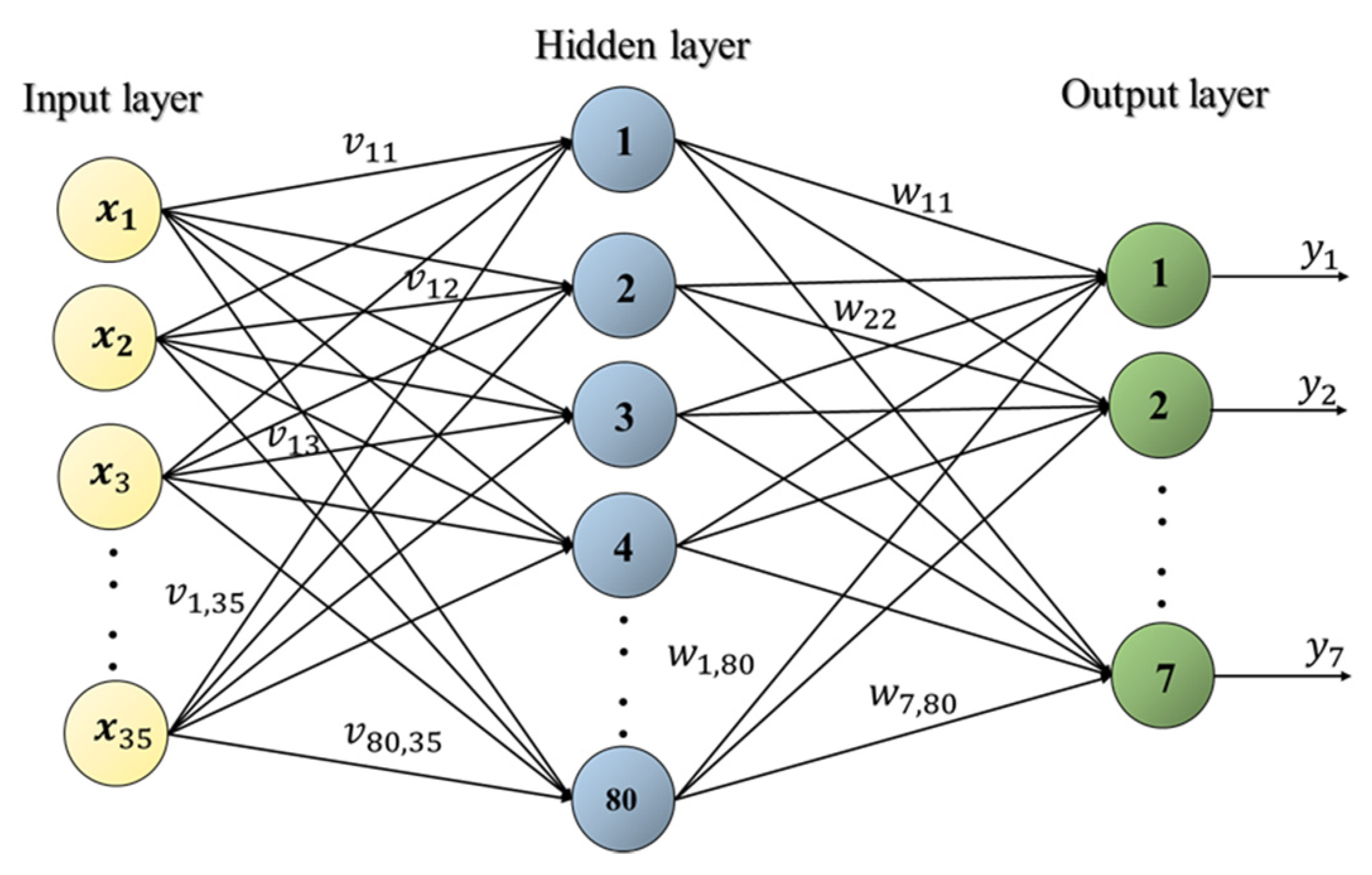
Applsci 10 00839 g001
Figure 2. The structure of BPN.
Applsci 10 00839 g002
Figure 3. (a) The finite element model. (b) The damaged scenario (the bracings was removed from the red circle).
Applsci 10 00839 g003
Figure 4. Detailed structure of the artificial neural network (ANN).
Applsci 10 00839 g004
Figure 5. (a) The training state. (b) Regression distribution of the training, test.
Applsci 10 00839 g005
Figure 6. Health index of damage on the first floor.
Applsci 10 00839 g006
Figure 7. Health index of damage on the sixth floor.
Applsci 10 00839 g007
Figure 8. Health index of damage for the third floor and the fourth floor.
Applsci 10 00839 g008
Figure 9. Health index of damage from the first floor to the third floor.
Applsci 10 00839 g009
Figure 10. Health index of damage from the fourth floor to the seventh floor.
Applsci 10 00839 g010
Figure 11. Health index of damage on the low floors.
Applsci 10 00839 g011
Figure 12. Health index of damage on the middle floors.
Applsci 10 00839 g012
Figure 13. Health index of damage on the high floor.
Applsci 10 00839 g013
Figure 14. A seven-story scale-down benchmark structure.
Applsci 10 00839 g014
Figure 15. Arrangement of velocity meter and mass block.
Applsci 10 00839 g015
Figure 16. The damage simulation: (a) the healthy condition; (b) the damaged condition.
Applsci 10 00839 g016
Figure 17. (a) The training state; (b) Regression distribution of the training, test.
Applsci 10 00839 g017aApplsci 10 00839 g017b
Figure 18. Health index of damage on the second floor.
Applsci 10 00839 g018
Figure 19. Health index of damage on the fourth floor.
Applsci 10 00839 g019
Figure 20. Health index of damage on the fifth floor and the sixth floor.
Applsci 10 00839 g020
Figure 21. Health index of damage from the first floor to the third floor.
Applsci 10 00839 g021
Figure 22. Health index of damage from the fourth floor to the seventh floor.
Applsci 10 00839 g022
Table 1. Damage cases and modal analysis.
Damage GroupDamage FloorsFrequency (Hz)
UndamagedNone3.25
One-story damage1F2.98
2F2.18
3F1.9
4F2.08
5F2.34
6F2.76
7F3.54
Two-story damage1&2F1.79
3&4F1.51
5&6F2.01
Three-story damage1&2&3F1.22
4&5&6F1.56
Multistory damage1&2&3&4F2.5
4&5&6&7F1.54
Table 2. Relationship between stiffness loss and health index.
Stiffness KHealth Index
K*1 (Health)1
K*0.70.7
K*0.350.35
K*00
Table 3. Parameters applied for training.
Training Parameters
Number of neurons80
Number of hidden layers1
Transfer functionLogsig
Epoch30,000
Max failure number0
TimeInfinite
Goal0
Min gradient1 × 10−7
mu0.005
mu_decrement0.1
mu_increment10
Max mu1 × 1010
Table 4. Diagnosis result of damage on the first floor (case 1).
Damaged FloorHealth IndexEvaluated Health IndexError (%)
1F00.0262.6%
2F 10.74425.6%
3F 10.79620.4%
4F 10.81218.8%
5F 10.9752.5%
6F 10.9366.4%
7F 10.982%
Table 5. Diagnosis result of damage on the sixth floor (case 2).
Damaged FloorHealth IndexEvaluated Health IndexError (%)
1F 10.9831.7%
2F 11.0373.7%
3F 10.9821.8%
4F 10.9881.2%
5F 11.0191.9%
6F00.0141.4%
7F 10.9237.7%
Table 6. Diagnosis result of damage for the third floor and the fourth floor (case 3).
Damaged FloorHealth IndexEvaluated Health IndexError (%)
1F 10.9960.4%
2F 10.9584.2%
3F00.0060.6%
4F00.0040.4%
5F 10.83516.5%
6F 10.9772.3%
7F 10.9970.3%
Table 7. Diagnosis result of damage from the first floor to the third floor (case 4).
Damaged FloorHealth IndexEvaluated Health IndexError (%)
1F00.033%
2F00.0181.8%
3F00.0474.7%
4F 10.9326.8%
5F 11.0090.9%
6F 11.055%
7F 10.9871.3%
Table 8. Diagnosis result of damage from the fourth floor to the seventh floor (case 5).
Damaged FloorHealth IndexEvaluated Health IndexError (%)
1F 10.9861.4%
2F 10.9940.6%
3F 11.0020.2%
4F00.0020.2%
5F00.0050.5%
6F0-0.0090.9%
7F0-0.0020.2%
Table 9. Diagnosis result of damage on the low floors (case 6).
Stiffness ReductionHealth IndexEvaluated Health IndexError (%)
1Fk*0.70.70.7858.5%
2Fk*0.70.70.88118.1%
3Fk*0.350.350.4015.1%
4Fk11.0464.6%
5Fk10.910%
6Fk10.9861.4%
7Fk11.0292.9%
Table 10. Diagnosis result of damage on the middle floors (case 7).
Stiffness ReductionHealth IndexEvaluated Health IndexError (%)
1Fk10.982%
2Fk10.9811.9%
3Fk*0.70.70.7333.3%
4Fk*0.350.350.350%
5Fk*0.350.350.3311.9%
6Fk11.0111.1%
7Fk10.9881.2%
Table 11. Diagnosis result of damage on the high floors (case 8).
Stiffness ReductionHealth IndexEvaluated Health IndexError (%)
1Fk10.9841.6%
2Fk11.0444.4%
3Fk10.9881.2%
4Fk110%
5Fk*350.350.3712.1%
6Fk*0.70.70.6891.1%
7Fk*0.350.350.3611.1%
Table 12. Damage cases and modal analysis.
Damage GroupDamage FloorsFrequency (Hz)
UndamagedNone3.34
One-story damage1F2.08
2F2.13
3F2.12
4F2.29
5F2.61
6F2.88
7F3.2
Two-story damage1&2F1.64
3&4F1.83
5&6F2.32
Three-story damage1&2&3F1.44
4&5&6F1.88
Multistory damage1&2&3&4F1.33
4&5&6&7F1.86
Table 13. Parameters applied for training.
Training Parameters
Number of neurons50
Number of hidden layers1
Transfer functionLogsig
Epoch30,000
Max failure number0
TimeInfinite
Goal0
Min gradient1 × 10−7
mu0.005
mu_decrement0.1
mu_increment10
Max mu1 × 1010
Table 14. Diagnosis result of damage on the second floor.
Damaged FloorHealth IndexEvaluated Health IndexError (%)
1F 110%
2F00.25725.7%
3F 110%
4F 110%
5F 110%
6F 10.88711.3%
7F 10.9574.3%
Table 15. Diagnosis result of damage on the fourth floor.
Damaged FloorHealth IndexEvaluated Health IndexError (%)
1F 10.81118.9%
2F 10.74425.6%
3F 10.991%
4F00.54854.8%
5F 10.62737.3%
6F 110%
7F 110%
Table 16. Diagnosis result of damage on the fifth floor and the sixth floor.
Damaged FloorHealth IndexEvaluated Health IndexError (%)
1F 110%
2F 110%
3F 110%
4F 110%
5F000%
6F000%
7F 10.46753.3%
Table 17. Diagnosis result of damage from the first floor to the third floor.
Damaged FloorHealth IndexEvaluated Health IndexError (%)
1F00.41741.7%
2F00.0565.6%
3F00.33833.8%
4F 10.74725.3%
5F 10.9534.7%
6F 10.9495.1%
7F 110%
Table 18. Diagnosis result of damage from the fourth floor to the seventh floor.
Damaged FloorHealth IndexEvaluated Health IndexError (%)
1F 110%
2F 110%
3F 10.68831.2%
4F00.20620.6%
5F00.0626.2%
6F000%
7F00.0151.5%
Table 19. The results of confusion matrix for the experimental verification.
Damaged FloorsRCMCSE
TPFPTNFN
1F5011
2F6010
3F4012
4F6100
5F5011
6F5011
7F5011
1&2F5020
3&4F5020
5&6F4021
1&2&3F4120
4&5&6F4030
1&2&3&4F3130
4&5&6&7F3040
Total643247
Accuracy89.8%
Precision95.5%
Recall90%

