A Wi-Fi FTM-Based Indoor Positioning Method with LOS/NLOS Identification

Abstract

In recent years, many new technologies have been used in indoor positioning. In 2016, IEEE 802.11-2016 created a Wi-Fi fine timing measurement (FTM) protocol, making Wi-Fi ranging more robust and accurate, and providing meter-level positioning accuracy. However, the accuracy of positioning methods based on the new ranging technology is influenced by non-line-of-sight (NLOS) errors. To enhance the accuracy, a positioning method with LOS (line-of-sight)/NLOS identification is proposed in this paper. A Gaussian model has been established to identify NLOS signals. After identifying and discarding NLOS signals, the least square (LS) algorithm is used to calculate the location. The results of the numerical experiments indicate that our algorithm can identify and discard NLOS signals with a precision of 83.01% and a recall of 74.97%. Moreover, compared with the traditional algorithms, by all ranging results, the proposed method features more accurate and stable results for indoor positioning.

1. Introduction

The importance of indoor positioning is reflected by the increasing requirements of location-based services (LBSs). Under such a background, global researchers have proposed a lot of indoor positioning methods based on different technologies, such as wireless fidelity (Wi-Fi) [1,2], Bluetooth [3], radio frequency identification (RFID) [4], computer vision [5], ultra-wideband (UWB) [6], infrared [7], and inertial navigation systems (INSs) [8], micro-electro-mechanical systems (MEMSs) [9], visible light [10,11], geomagnetic fields [12,13], and pseudolites [14,15], among others.

Among these methods, methods based on Wi-Fi have attracted much attention due to their wide distribution. They can be defined as fingerprint-based methods [16] and distance-based methods. The former can reach an accuracy of about 2 m and needs to construct a fingerprint database at the offline stage, which costs more labor and time. The latter can calculate the distance between the transceivers according to the received signal strength indicator (RSSI), then use the least square (LS), trilateral positioning, or other algorithms to derive the location. However, the RSSI, when collected at a fixed place, could be influenced by device heterogeneity and non-line-of-sight (NLOS) errors, so it is difficult to use widely.

This phenomenon did not change until 2016. The fine timing measurement (FTM) protocol has been standardized by the Institute of Electrical and Electronics Engineers (IEEE) 802.11-2016 and can provide meter-level positioning accuracy [17] through time of flight (TOF) echo technology [18]. However, just like many other ranging measurements, such as UWB [19,20] and Global Positioning System (GPS) [21,22], one of the major challenges for positioning is the mitigation of NLOS effects. If the direct path between a fixed terminal (FT) and a mobile terminal (MT) is obstructed, the time of arrival (TOA) of the signal to the FT will be delayed, which will introduce a positive bias. The use of such TOA estimates may significantly degrade accuracy during the positioning process. Hence, it is necessary to identify NLOS signals.

NLOS identification has been extensively discussed for UWB signals [23], while it has rarely been discussed for Wi-Fi signals, as only RSSIs rather than more detailed channel state information (CSI) data can be collected from Wi-Fi devices with mobile phones. Therefore, elucidating how to identify NLOS signals using RSSI has become one of the major difficulties of this work. Joan Borras [24] formulated a theoretical framework where various theoretical tests were developed for known and unknown models of NLOS errors. Ke Han [25] calculated the distance between the coordinates of the FT and that of MT, which were obtained via pedestrian dead reckoning (PDR). Then, the obtained values were used to build two Gaussian models to identify line-of-sight (LOS) signals and NLOS signals, respectively. Considering that RSSIs will attenuate as they pass through different materials, this method may perform poorly in some environments. Jo [26] determined LOS signals according to the difference of RSSI between a 2.4 GHz signal and that of a 5 GHz signal. However, the new FTM protocol that supports Wi-Fi devices can only send single-frequency signals, so this method is not suitable. Except for identification methods based on received multipath signals, some methods have been designed using the overall mobile network as their basis. Chen [27] used various combinations of ranging results to evaluate the positioning and residual of an MT. The combination with a smaller residual has a larger chance of obtaining a higher accuracy. Some other NLOS error mitigation methods using the mobile network have been reported in [28,29,30,31,32,33,34].

This study proposes a Wi-Fi FTM-based indoor positioning method that uses LOS/NLOS identification. A Gaussian model has been built in order to identify NLOS signals. LOS signals are used to calculate the locations of an MT with an LS algorithm. Based on the newest Wi-Fi technology, this method is suitable for future Wi-Fi devices. Moreover, the identification model built by this method is more suitable for complex indoor environments.

The contributions of this work are summarized as follows:

(1)

In order to discard the NLOS error, an identification model is proposed. Differing from other Gaussian-based models, which have established two models for LOS and NLOS, the model presented here only needs to establish one model in order to adapt to the complex indoor environment.

(2)

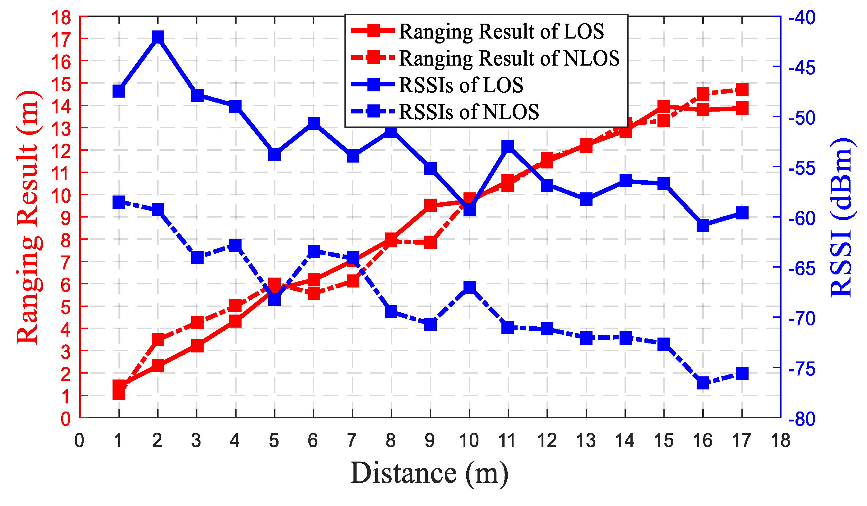
To solve the difficulty of setting parameters, we have researched and fit the relation between RSSI and ranging results, achieving adaptive settings.

The remainder of this paper is organized as follows: Section 2 introduces the theoretical framework, including the round-trip time (RTT)-based ranging model and the propagation and attenuation of Wi-Fi signals. Section 3 introduces the proposed method, including the construction of the Gaussian model for identification and the iterative least squares algorithm. Section 4 describes the experimental results by the proposed method. Section 5 presents a conclusion and points out areas for future work.

2. Theoretical Framework

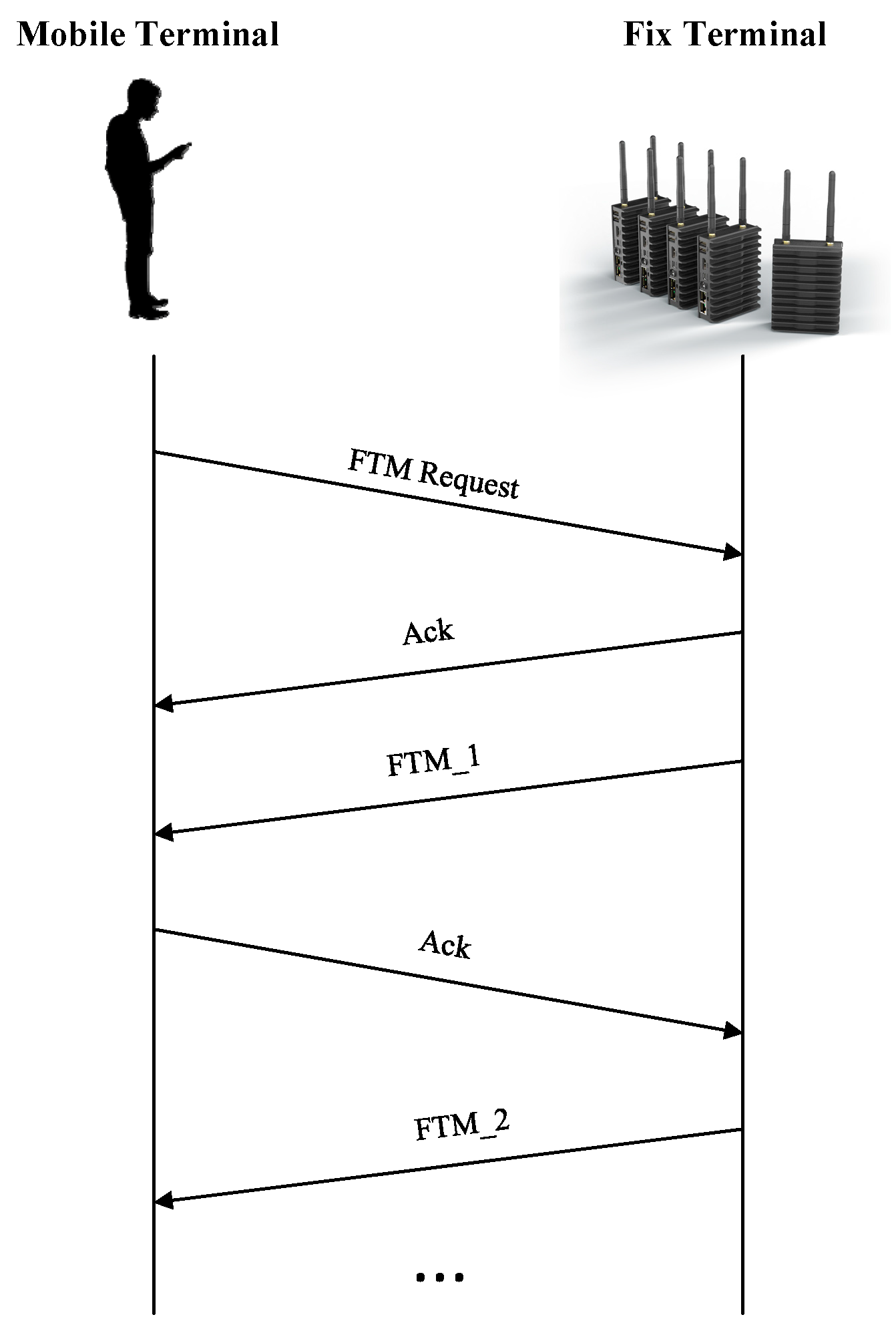
2.1. RTT-Based Ranging Model

Here, TOF echo technology is used in the Wi-Fi FTM protocol and makes the RTT based ranging more convenient [18]. This new technology determines the distance according to the RTT of a Wi-Fi FTM pulse from an MT to an FT. Accordingly, it can eliminate the time synchronization errors in the time of arrival (TOA)/time difference of arrival (TDOA)-based ranging, with no need to synchronize the times of the FT and MT. The whole procedure of ranging is shown in Figure 1. It shows that a mobile phone is used as an MT to send an FTM request to FTs supporting the FTM protocol. After an FT receives the request, an Acknowledgement (ACK) signal is sent from the FT to the MT. After that, several FTM feedback signals are sent from the FT to the MT, where the mean RTT can then be calculated. The time information can be expressed as follows:

$$t_{ACK}=t_{request}+\frac{2}{c}{\Vert p_{MT}-p_{FT}\Vert }_2+t_D+e_{NLOS}$$

(1)

where $t_{request}$ and $t_{ACK}$ are the times for when the request was sent from the MT and when the ACK signal arrives at MT; $p_{MT}$ is the location of the MT when the FTM request is sent; $p_{FT}$ is the location of the FT when the MT receives the FTM request; $t_D$ is standard time deviation between the MT and the FT; $e_{NLOS}$ is the time delay error caused by the NLOS effect; and c is the speed of light. Hence, the distance can be calculated by Equation (2):

$$\rho ={\Vert p_{MT}-p_{FT}\Vert }_2=d_{RTT}-d_D-d_{NLOS}$$

(2)

where $d_{RTT}$ is the ranging result; $d_D$ is the ranging error caused by standard time deviation, as shown in Equation (3); and $d_{NLOS}$ is the ranging error caused by the NLOS effect. The ranging error $d_D$ not only includes a fixed time delay error, a device error, and a start error, but also is influenced by the distance of pulse propagation and other environmental factors [35], which can be expressed as follows:

$$d_D=e_n+\phi (s)+\epsilon$$

(3)

where $e_n$ is the constant error caused by the fixed time delay error, the device error, and the start error; $\phi (s)$ is the error formed by different ranging results, which can be seen as a polynomial function related to the ranging results; and $\epsilon$ is the system noise. It can be seen that the standard time deviation error of the equipment needs to be determined and calibrated to provide more precise ranging results.

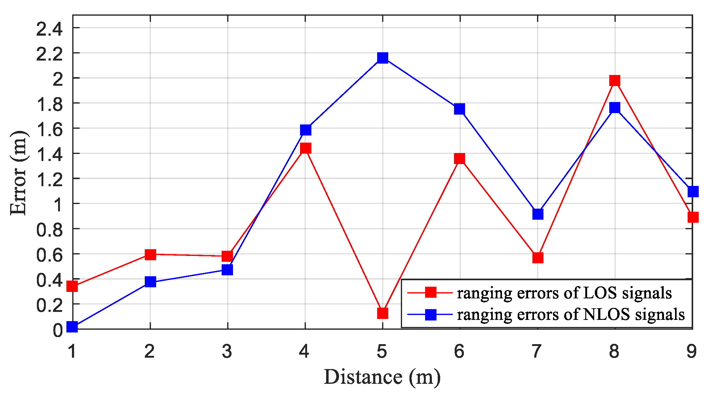
2.2. Propagation of Wi-Fi Signals

With wave-particle duality, electromagnetic waves are the method of Wi-Fi propagation, which exhibit both particle properties and wave properties during propagation [36,37]. In a wide space, electromagnetic waves are only transmitted directly without obstacles. While in an indoor environment, the propagation characteristics will change due to the existence of various objects, causing reflection and diffraction, etc. In addition, electromagnetic waves have a certain penetration ability and can spread across walls. As a result, the actual propagation process of electromagnetic waves is varied and complex.

The propagation of electromagnetic waves follows the ‘skin effect’ [38]. That is, when there is an alternating current or alternating electromagnetic field in a conductor, the current distributes unevenly and concentrates in the ‘skin’ part of the conductor, that is, the current is concentrated on the thin layer of the outer surface of the conductor. As a result, the resistance of the conductor is increased, and its power loss is also increased. When an electromagnetic wave carrying a signal passes through some media, it is restricted by the skin effect, such that a part of the electromagnetic wave stays on the surface of the media and cannot completely pass through the media. The better the conductivity of the medium, the more obvious the effect of blocking in the electromagnetic wave is, and the more obvious the attenuation of the signal intensity is.

Table 1. Signal attenuation through different media.

Obstacle	Reinforced Concrete Wall	Plasterboard Wall	Wooden Door	Metal Door	Glass Window
Signal Attenuation Value (dBm)	15–16	3–5	3–5	10–12	6–8

presents the signal attenuation of electromagnetic waves with a frequency of 2.4 GHz when crossing various common obstacles in indoor buildings. It can be obtained through observation that the better the conductivity of an obstacle is, the more obvious signal attenuation will be.

Electromagnetic waves will wear out when propagating in air. The loss in free space is mainly caused by the air’s own propagation and the scattering and refraction of fine dust particles. In the case of no obstacles in the air, the propagation of electromagnetic waves can be expressed as per Equation (4) [39], where d is the distance from the MT to the FT; $d_0$ is the reference distance; $L(d)$ is the received power of the MT when the distance from the FT is d; $L(d_0)$ is the received power when the distance from the FT to the MT is 1 m; $\eta$ is the attenuation coefficient; and k is the shadowing factor, obeying a Gaussian distribution with a mean of 0. Since the model is in the case of LOS, k is 0.

$$L(d)=L(d_0)+10\cdot \eta \cdot lg(\frac{d}{d_0})+k$$

(4)

3. The Proposed Indoor Localization Method

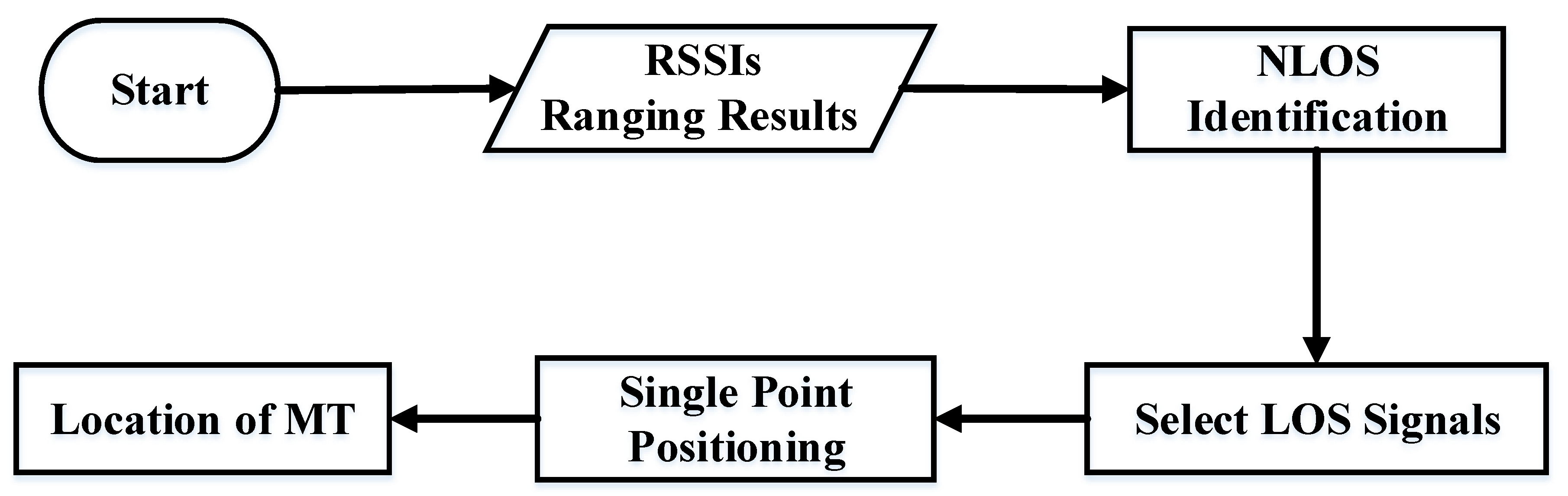
3.1. Overall Structure of the Proposed Method

Figure 2 shows the procedures of the proposed positioning method. The ranging results and RSSIs are collected from the FTs and then input into the LOS/NLOS identification model. Then, the model identifies NLOS signals and only outputs the LOS ranging results. If the number of LOS ranging results is greater than the minimum number required for positioning, the LOS ranging results are used as the input of the single point positioning to calculate the location of the MT. If the number of LOS ranging results is less than the minimum number, all the ranging results, including LOS and NLOS, will be used as the input of the single point positioning to derive the location.

3.2. The Identification Model of LOS/NLOS

Figure 3 shows the ranging results (the red solid line and the dotted line) and RSSIs (the blue solid line and the dotted line) collected at different distances from FTs under both NLOS and LOS conditions. Here, we have placed Wi-Fi devices in an open corridor and in a closed room, then collected RSSIs and ranging results at 1 m intervals in the corridor. The sampling time was 30 s, the sampling frequency was 5 Hz, and the sampling device was a Pixel 3 mobile phone. The solid line denotes the results from a corridor and the dotted line denotes the results from a closed room. It can be seen that the LOS and NLOS ranging results are similar at any distance, but the RSSIs are quite different. This is due to the principle of electromagnetic wave propagation. RSSIs mainly reflect the amplitude of the electromagnetic wave. When electromagnetic waves travel through walls, some particles will not pass through walls, and the amplitude will significantly reduce, such that the RSSI will also be reduced [38]. The ranging results mainly reflect the time of propagation. When the electromagnetic waves pass through the wall, their speed will decrease. However, due to the small thickness of the wall and the high electromagnetic velocity, the impact on the time of propagation and ranging result is small. Under such conditions, the ranging results are not obvious when compared with those of an RSSI. The LOS/NLOS identification model was designed based on this phenomenon.

According to Section 2.2, the attenuation of the RSSIs was greatly affected by the conductivity of obstacles. In the complex indoor environment, it is difficult to model the relationship between the distance and RSSI. Therefore, differing from the literature [24,25,40], where two models have been built under LOS and NLOS conditions, respectively, this paper’s identification model was built in the line-of-sight condition, which could output probability with a large difference according to the condition of the signal.

Most existing works [41,42,43] use a Gaussian distribution to model the randomness of RSSI, and consequently, in this paper, a Gaussian model was established to calculate the probability of LOS by Equation (5), as shown in Figure 4. The parameters of the model were determined by ranging results, and the inputs of the model were the RSSIs of the FTs. According to the maximum likelihood method, μ is the mean of the RSSI and σ is the variance of the RSSI in Equations (6) and (7), where $RSS{I}_d^i$ is the RSSI collected at the distance d; N is the number of RSSI collected. The determination of $\mu$ and $\sigma$ is described below in detail. After the parameters were determined, the probability could be determined by inputting the RSSI into the Gaussian model. Then, the probability was compared with the threshold $\theta$. If the probability is greater than the threshold, the current signal is a LOS signal, and if it is less than, it is not.

$$P_{LOS}(RSSI)=\frac{A}{\sqrt{2\pi }\sigma }\ast exp\left(-\frac{{(RSSI-\mu )}^2}{2{\sigma }^2}\right)$$

(5)

$$\mu =\frac{1}{N}{\displaystyle \sum _{i=1}^{N}RSS{I_d}^{(i)}}$$

(6)

$${\sigma }^2=\frac{1}{N}{\displaystyle \sum _{i=1}^N{(RSS{I_d}^{(i)}-\overline{RSS{I}_d})}^2}$$

(7)

3.2.1. The Determination of d

In the paper, it was assumed that the ranging results could reflect the true distance to a certain extent. Therefore, we needed to evaluate the accuracy of the ranging results based on Wi-Fi RTT. As shown in Figure 5, a tester collected the ranging results of the FTs at each grid point. Here, the grid side length was 1 m, the sampling time was 30 s, and the sampling frequency was 5 Hz. The MT and FTs were basically at the same height during sampling. The ranging accuracy is shown in Figure 6. The red and blue solid lines are the ranging errors of the LOS signals and NLOS signals, respectively. Through calculation, the average ranging error of LOS signals was 0.87 m and the variance was 0.36 m. The average ranging error of the NLOS signals was 1.16 m and the variance was 0.54m. It can be seen that RTT-based ranging results can accurately reflect the true distance between the transceivers. At the same time, the ranging accuracy and stability of the LOS signals were better than those of the NLOS signals.

3.2.2. The Determination of μ

$\mathsf{\mu }$ is the mean of RSSIs collected when the distance between an MT and FT is determined. According to the propagation model of electromagnetic waves, in Equation (5), the true distance is exponential with RSSI, so the exponential model was used to fit the ranging results and RSSIs.

A Wi-Fi device was arranged at a fixed point as the FT. The experimenter walked in a straight line with the mobile phone within 23 m from the FT. One thousand, eight hundred groups of ranging results and RSSIs were collected and used as training data. The collected ranging results and RSSIs were used as training data. The fitting of the single exponential model is shown in Figure 7a. It can be seen that fitting over 15 m performs poorly. Here, the mean square error (MSE) was used to evaluate the fitting, calculated as per Equation (8), where N is the number of RSSI used for the fitting; $RSS{I}^{(i)}$ is the i-th RSSI for the fitting; and $RSS{I}_{fit}^{(i)}$ is the i-th fitting result. By calculating the MSE of the fitting from 0 m to a different distance, as shown in Figure 7b, it was found that within 0–15 m, as the distance increases, the training data increase, and the MSE decreases. Between 15 and 20 m, the MSE becomes larger, and the fitting effect is not good. Over 20 m, the MSE tends to be stable. It can be concluded that the RSSIs collected at the distance over 15 m have a different tendency from those collected within 15 m. Therefore, the ranging result RSSI model was changed into a double exponential model to calculate μ, as shown in Equation (9). The data in the range of 0–15 m and 15–25 m were fitted, respectively. The result of fitting using the double exponential model is shown in Figure 7c. The MSE of the fitting, using the double exponential from 0 m to different distances, is shown in Figure 7d. It can be seen that the MSE at different distances is lower than that of the single exponential, except at a distance of 4 m. The average MSE of the single exponential model was 4.85 dBm², and that of the improved double exponential model was 4.15 dBm². Therefore, the double exponential model is more in line with the ranging result–RSSI relationship.

$$MSE=\frac{1}{N}{\displaystyle \sum _{i=1}^N(RSS{I}^{(i)}-RSS{I}_{fit}^{(i)})}$$

(8)

$$\mu =\{\begin{array}{cc}{a}_1+b_1\ast lg(d)& d<15m\\ a_2+b_2\ast lg(d)& d\ge 15m\end{array}$$

(9)

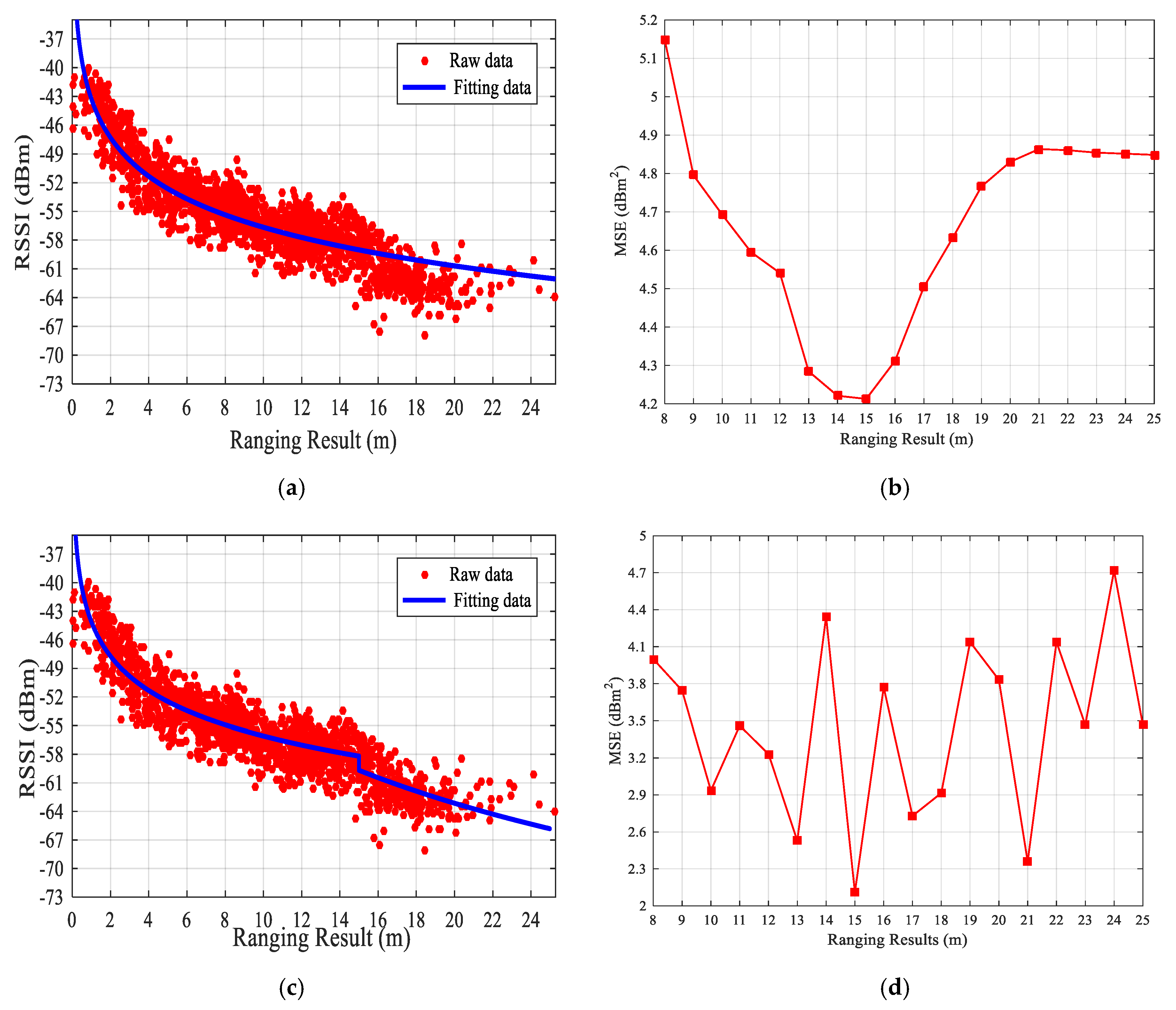
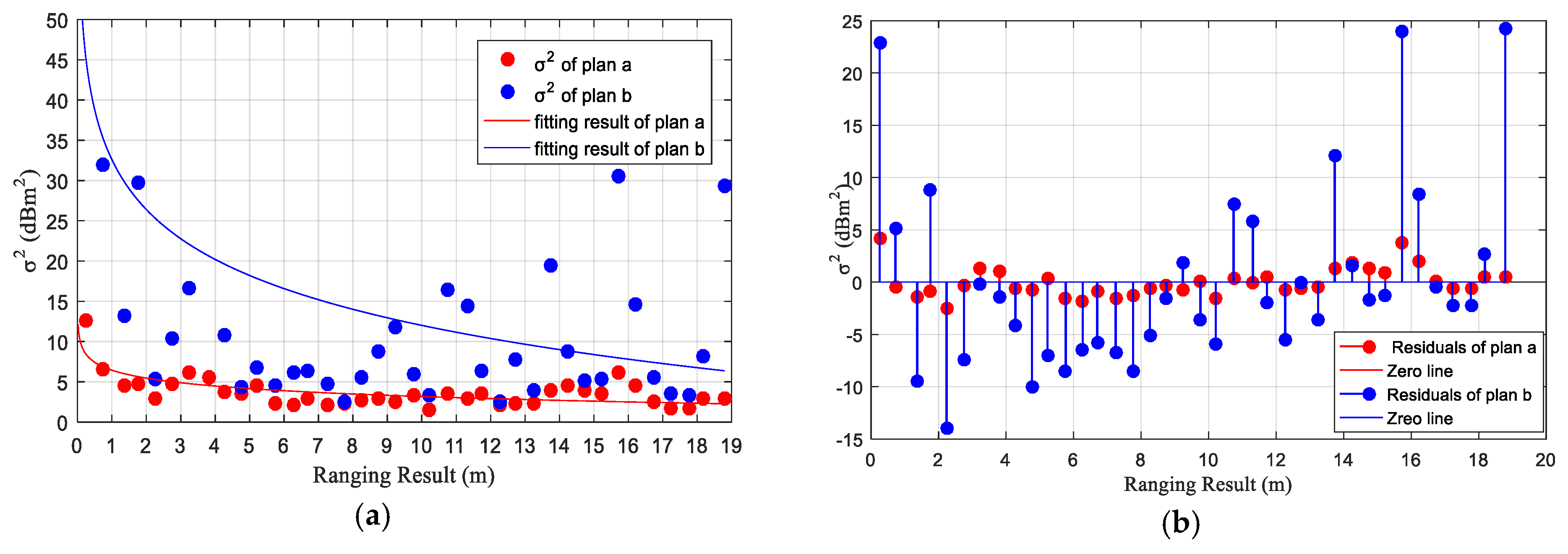
3.2.3. The Determination of σ

$\mathsf{\sigma }$ is the variance of RSSIs collected at a fixed point. In the literature [24,25], the variances of RSSIs collected at different distances have traditionally been set as a fixed value. According to the analysis in the second section, we assumed that the variances of RSSIs at different distances were different. For this reason, the variances were calculated, as shown in

Table 2. Variance of RSSIs at different distances.

Distance Range (m)	0–3	3–6	6–9	9–12	12–15	15–18
σ (dBm)	3.48	2.34	1.66	1.69	1.74	1.74

. It can be seen that the variance decreased by about 1 dBm² from 0 to 6 m, while it nearly did not change from 6 to 18 m. According to the trend of change, the exponential function was used to fit the variances and ranging results. To verify if the function was suitable, the sum of squares due to error (SSE) and coefficient of determination (R-square) of the fitting result was compared with that found by other functions, including the Fourier, Gaussian, linear fitting, polynomial, rational, and sum of sine functions, shown in the

Table 3. Sum of squares due to error (SSE) and coefficient of determination (R-square) values of the different fitting functions.

Fitting Function	SSE (dBm2)	R-Square Value
Our Model	72.77	0.48
Fourier	85.70	0.40
Linear Fitting	99.85	0.30
Polynomial	115.13	0.19
Rational	92.79	0.35
Sum of Sine	115.14	0.19

. SSE and R-square can be calculated by Equation (10) and Equation (11), where $\overline{RSSI}$ is the average of RSSI. The smaller the SSE or the bigger the R-square, the better the fitting results will be. It can be seen that from both the SSE and R-square that the exponential function is more suitable.

$$SSE={\displaystyle \sum _{i=1}^N(RSS{I}^{(i)}-RSS{I}_{fit}^{(i)})}$$

(10)

$$R-square=\frac{{\displaystyle \sum _{i=1}^N(\overline{RSSI}-RSS{I}_{fit}^{(i)})}}{{\displaystyle \sum _{i=1}^N(\overline{RSSI}-RSS{I}^{(i)})}}$$

(11)

For the fitting, a large amount of RSSIs with the same ranging results should be obtained. However, due to different ranging results, a credible variance was hard to achieve. The ranging results were divided into several 0.5 m-long ranges. Next, all the training data were put into the corresponding range according to the ranging results. Then, the average of the ranging results and the variances of RSSIs in each range were calculated and used as the input of the fitting. The variances were calculated by the following two methods:

(a)

The variances of RSSIs were directly calculated, according to Equation (7).

(b)

All the RSSIs were counted in a certain interval and the probabilities of each RSSI were calculated. Then, the Gaussian regression was performed on the probability and the corresponding RSSI. σ of the Gaussian model was taken as the σ of the current distance.

After the $\sigma$ values were determined, the ranging results and $\sigma$ values were fitted to generate a ranging result-based σ model. Figure 8 shows the fitting results of methods A and B. The red dot is the variance calculated by method A, while the blue point is the variance calculated by the other method. The fitting results and raw data are shown in Figure 8a, and the residuals of the two methods are shown in Figure 8b. It can be seen that variances calculated by method B fluctuate largely, which might be caused by over-fitting. In the range of 0–4 m, the variance of method B is higher than 15. Table 1 shows that the attenuation of RSSI caused by the reinforced concrete is about 15 dBm, so that when the variance is higher than 15, the output probability of LOS and NLOS is similar, which may make the set of threshold and identification difficult. Furthermore, as shown in Figure 8b, the fitting result of method A is better than method B, as the sum of square due to error (SSE) of method A is much smaller than that of method B. Hence, method A was used to calculate the variance used for the later fitting.

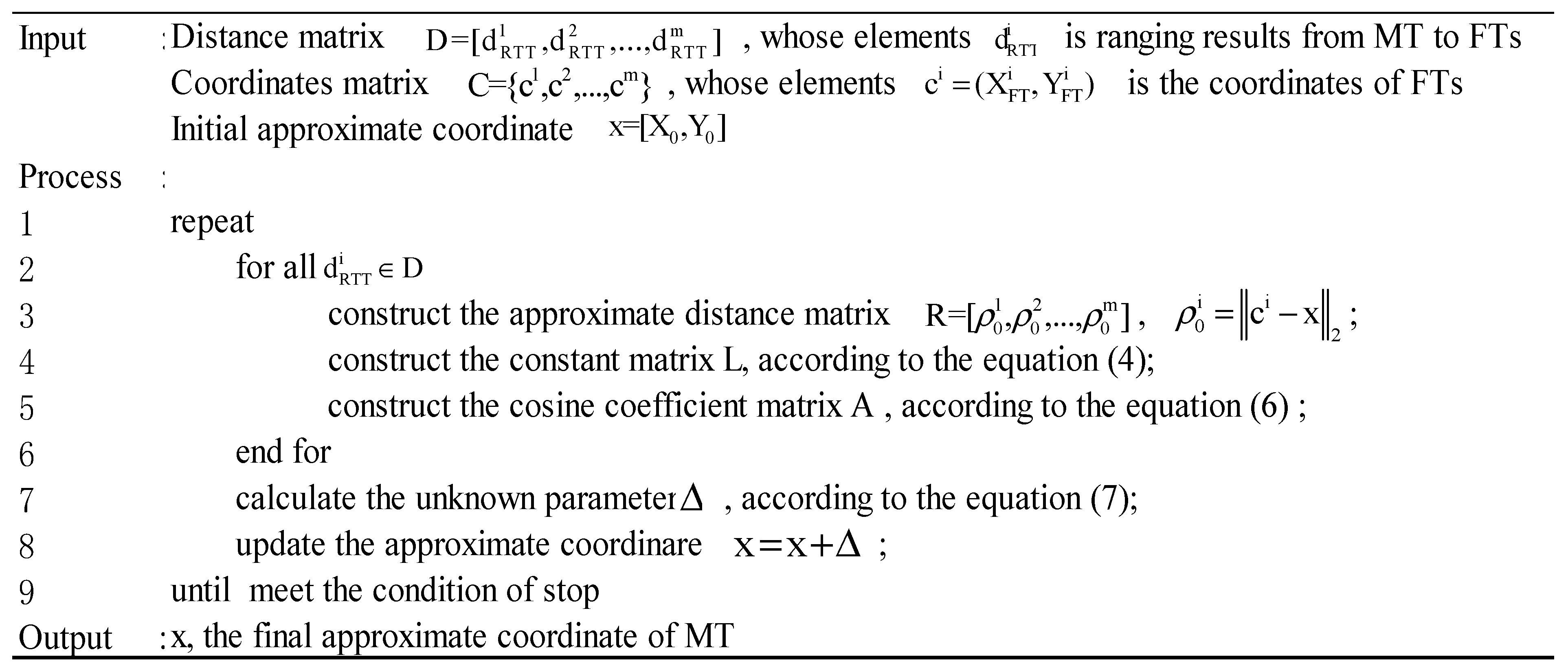
3.3. Single Point Positioning

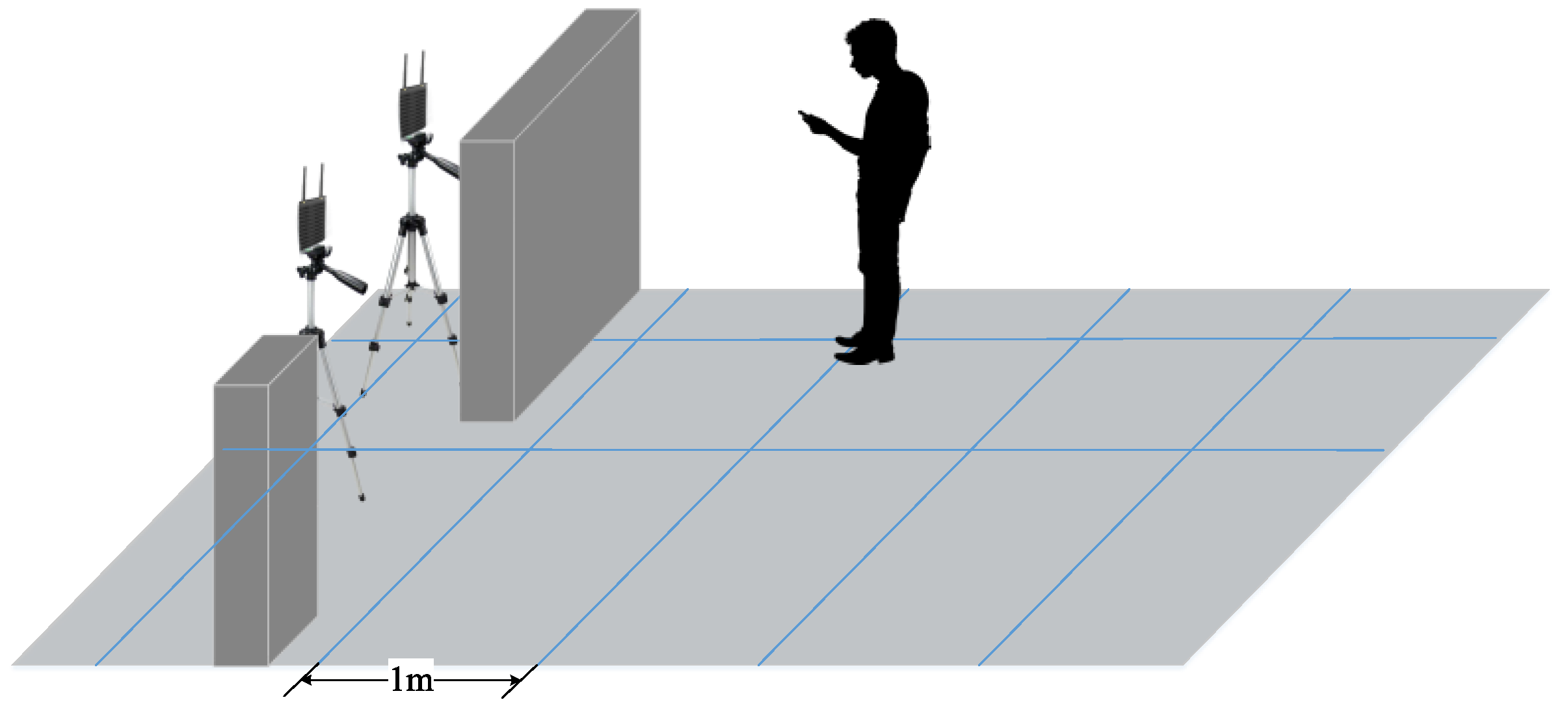
If the number of the ranging results was more than 2 after filtering, the LS algorithm was used for the single point positioning. The observation equation for the ranging results can be expressed as follows:

$$d_{RTT}^i={\rho }^i+d_D^i+d_{NLOS}^i$$

(12)

In the equation, $d_{RTT}^i$ is the ranging result collected from the i-th FT, ${\rho }^i$ is the Euclidean distance between the i-th FT and the MT, $d_{NLOS}^i$ is the ranging error caused by the NLOS error from the i-th FT; and d is the ranging error caused by the standard time deviation. According to Equation (12), we can derive the error observation as follows:

$$V^i={\rho }^i+d_D^i+d_{NLOS}^i-d_{RTT}^i$$

(13)

Assuming that the approximate coordinate of MT is X = (X₀, Y₀) and that the Euclidean distance from the coordinate of the i-th FT to the approximate coordinate of MT is ρ0, the Taylor series of the above formula is:

$$V^i={\rho }_0^i+\frac{X_0-X_{FT}^i}{{\rho }_0^i}dX+\frac{Y_0-Y_{FT}^i}{{\rho }_0^i}dY+d_D^i+d_{NLOS}^i-d_{RTT}^i$$

(14)

If we set the following:

$$L^i=d_{RTT}^i-{\rho }_0-d_D^i-d_{NLOS}^i$$

(15)

Then the equation could be changed as follows:

$$V^i=\frac{X_0-X_{FT}^i}{{\rho }_0^i}dX+\frac{Y_0-Y_{FT}^i}{{\rho }_0^i}dY-L^i$$

(16)

where dX and dY are the corrections of the approximate coordinates of MT, and $X_{FT}^i$ and $Y_{FT}^i$ are the two coordinate values of the i-th FT. Thus, Equation (14) can be expressed in a matrix form as follows:

$$\underset{m\times 1}{{\displaystyle V}}=\underset{m\times 2}{{\displaystyle A}}\times \underset{2\times 1}{{\displaystyle \Delta }}\times \underset{m\times 1}{{\displaystyle L}}$$

(17)

where m is the number of ranging results after filtering; V is the vector of the correction of ranging results; L is observation error constant matrix; $\mathsf{\Delta }$ is an unknown parameter in Equation (15); and A is the cosine coefficient matrix in Equation (19).

$$\Delta =[dX,dY]$$

(18)

$$A^i=[\frac{X_0-X_{FT}^i}{{\rho }_0},\frac{Y_0-Y_{FT}^i}{{\rho }_0}]$$

(19)

The error observation equation can be established using the ranging results from different FTs, and then the parameters of the coordinate can be obtained by solving the equation with the least square method, as shown in Equation (20).

$$\Delta ={(A^{T}A)}^{-1}\times A^T\times L$$

(20)

The pseudocode of single point positioning is shown in Figure 9. The observation equation was constructed using the inputs to calculate $\mathsf{\Delta }$. Through iteration, $\mathsf{\Delta }$ gradually approached 0, where the approximate coordinate of MT was gradually steady. When $\mathsf{\Delta }$ was smaller than a threshold or the iteration number was more than a threshold, the iteration could meet the condition of stopping.

4. Experiment

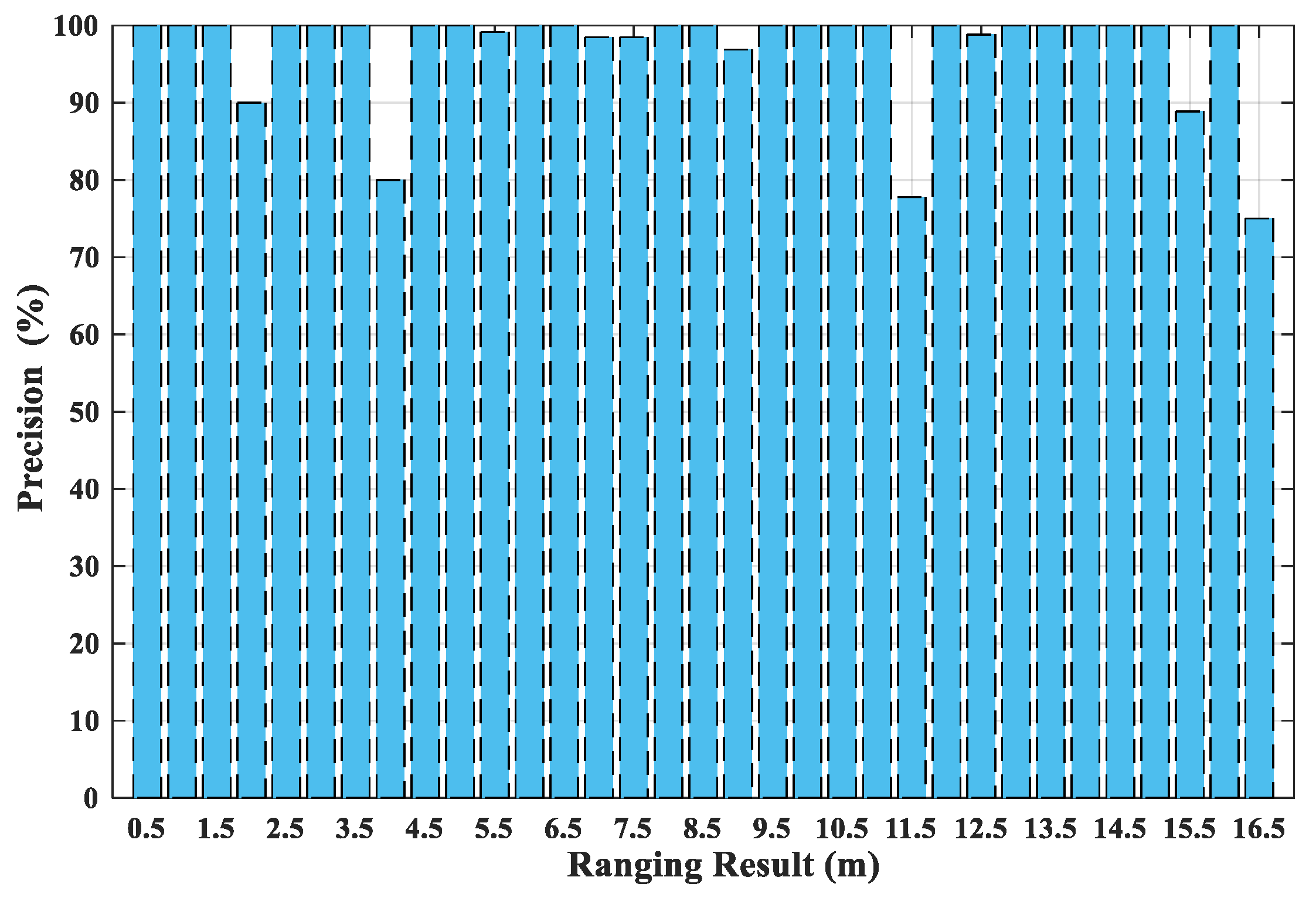
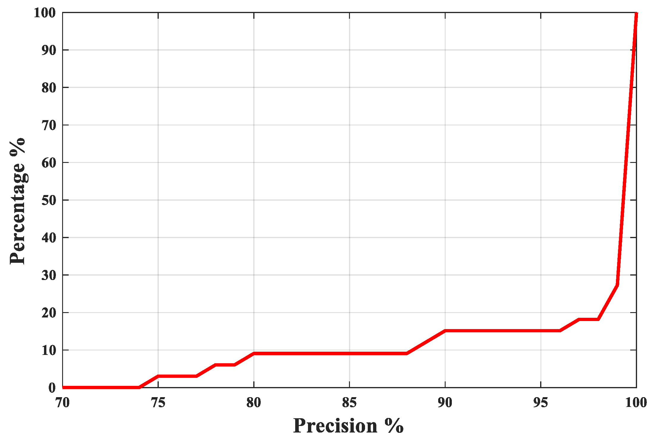
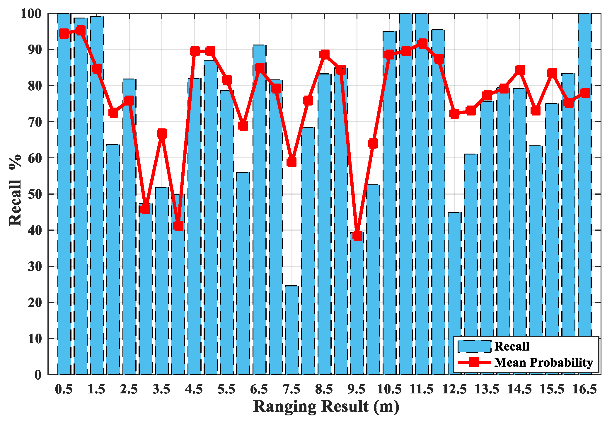
4.1. Evaluation of the Identification Model

The performance of the identification model was evaluated. A Wi-Fi device was set in the corridor, and the experimenter walked at a constant speed in the corridor and room separately with a mobile phone to collect the RSSIs and ranging results. The data collected in the corridor were seen as LOS data, while those collected in the room were seen as NLOS data. A group of data consisted of an RSSI and a ranging result. A total of 8360 groups of data were collected, among which 1800 groups were used for training and 6560 groups were used for testing. The training data acquisition time was only one day away from that of the testing data, and the training data did not participate in the test.

The identification of NLOS/LOS was a binary problem, so precision and recall were utilized to evaluate the model. They were calculated by Equations (21) and (22), respectively, where the TP (true positive) is the number of LOS signals that were accurately identified, FP (false positive) refers to the number of NLOS signals identified as LOS signals, and FN (false negative) points to the number of LOS signals identified as NLOS signals. All the data were divided into different ranges according to the ranging results in order to evaluate the precision and recall at different distances. Here, 3280 groups of LOS data and 3280 groups of NLOS data were used to test the precision, while 3280 groups of LOS data were used to test the recall. The model output the LOS/NLOS recognition results, then TP, FP, and FN were counted to calculate the precision and recall of each interval. In this experiment, the threshold θ of the model was set as 0.7.

$$P=\frac{TP}{TP+FP}$$

(21)

$$R=\frac{TP}{TP+FN}$$

(22)

Figure 10 shows the precision at different ranges. Through calculation, the average precision was 97.08% and the MSE was 0.07. Figure 11 shows the cumulative distribution of precision. All precisions were higher than 70%, 9.09% of which were lower than 85%, and 15.15% of which were lower than 95%. It can be seen that the precision of the model is poor at some ranges, which might be caused by the poor fitting of the ranging result and RSSI.

The recalls and mean probabilities at different ranges are shown in Figure 12, where the value of the blue column is roughly the same as that of the red line. It can be seen that the set of θ could distinguish LOS signals and NLOS signals. However, through calculation, the average recall was only 74.97% and the MSE was 0.2. Figure 13 shows the cumulative distribution of recalls. Here, 24.24% of the recalls were lower than 60%, and 51.52% of them were lower than 80%, indicating that the model often misjudges some LOS signals.

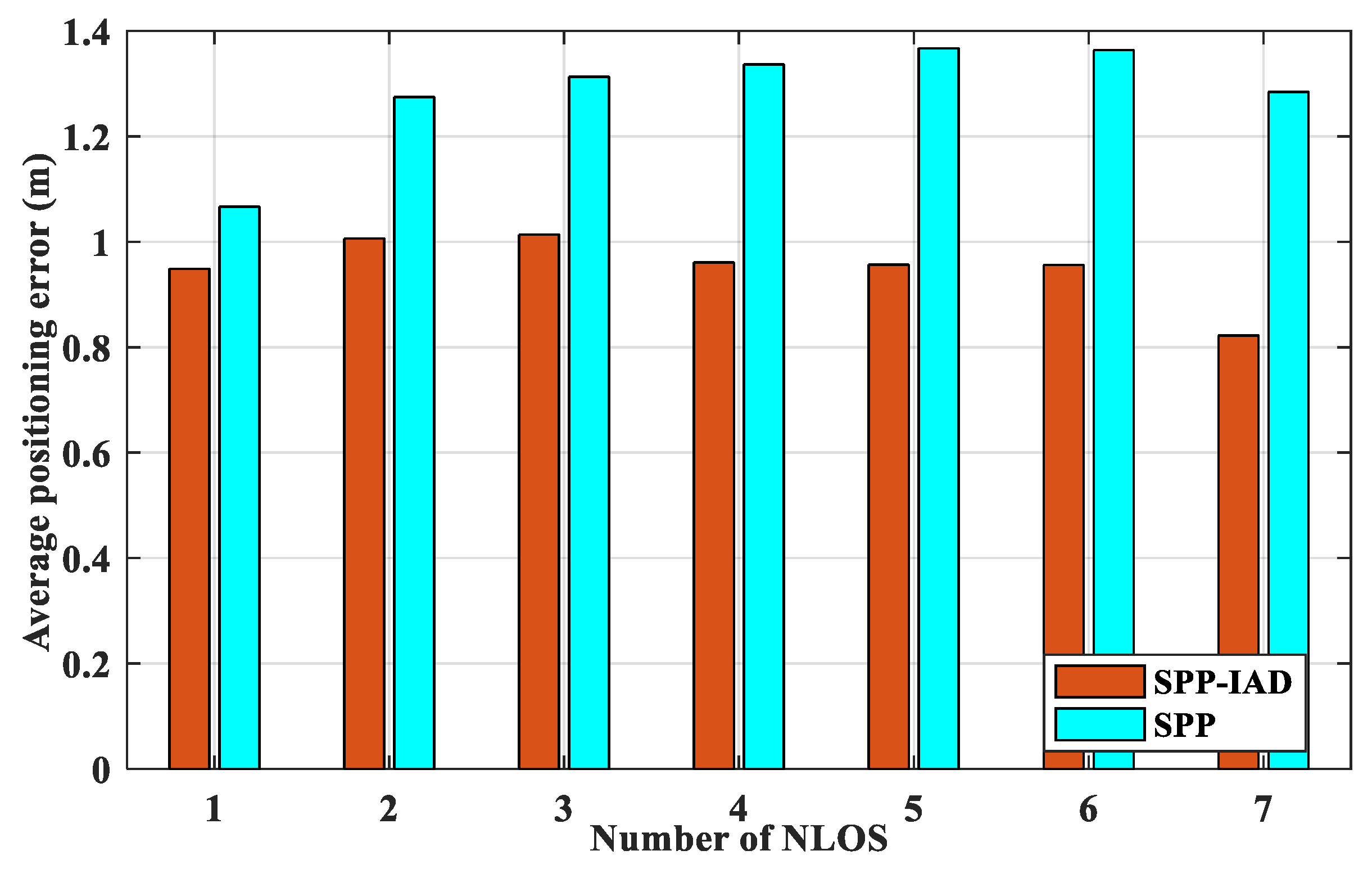
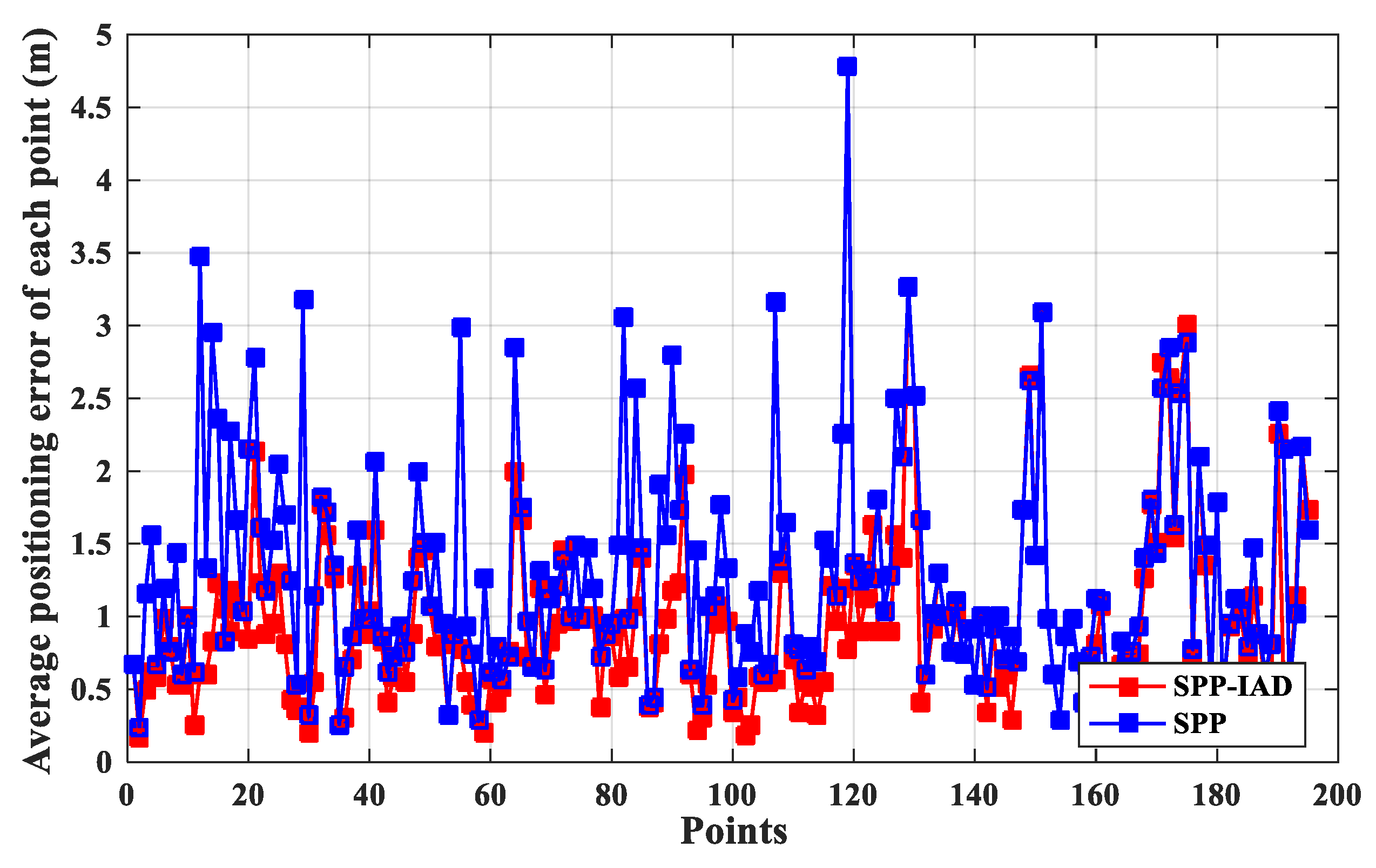
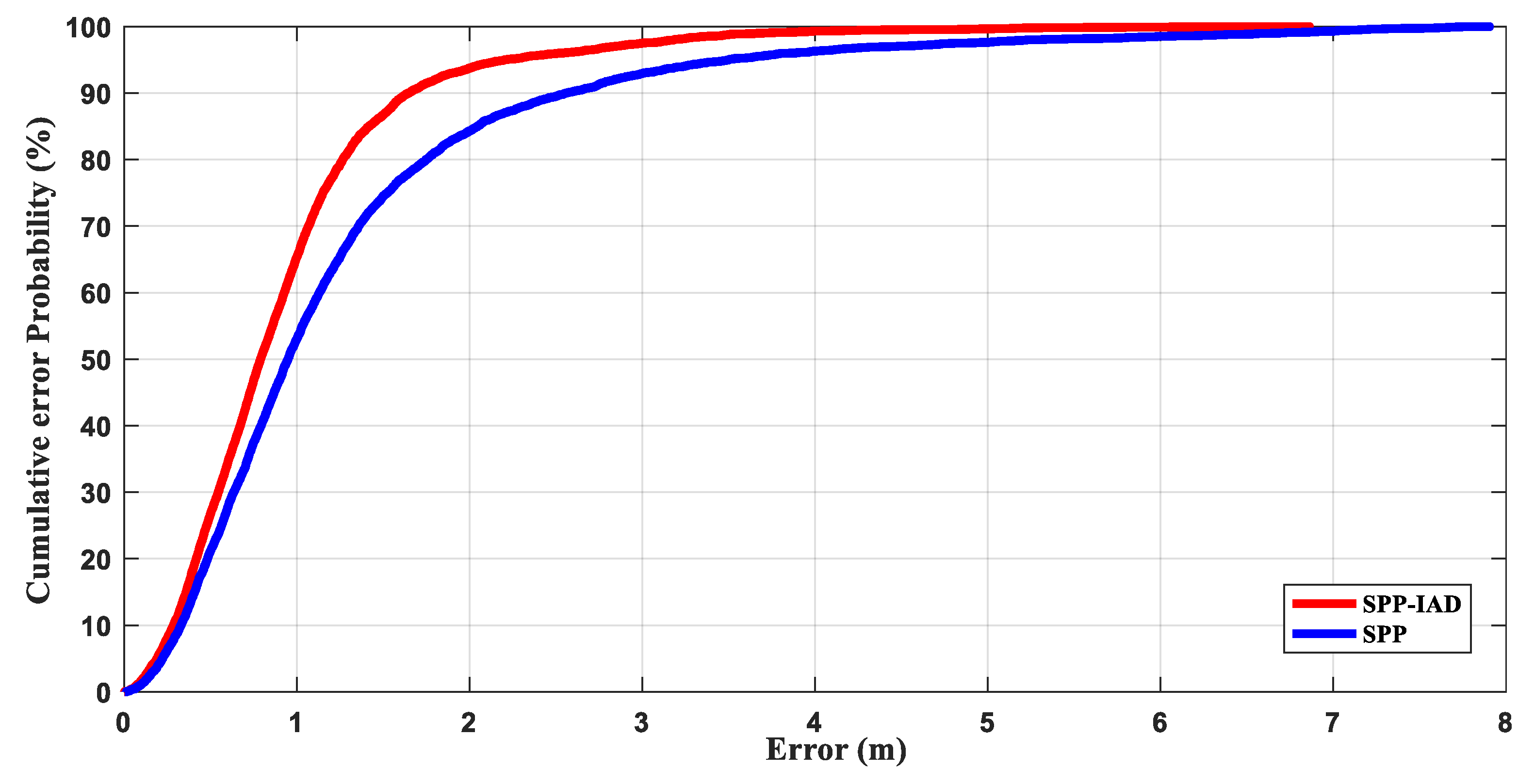
4.2. Evaluation of Proposed Positioning Method

The experimental environment is shown in Figure 14, which includes two rooms and a corridor adjacent to each other. Both of the rooms were 19.05 m long and 5.83 m wide, while the corridor was 19.51 m long and 1.74 m wide. Totally, 10 FTs were positioned on a tripod with a height of 1.3 m. Among them, 8 were placed in two rooms on average, where 3 were positioned in the corridor, marked with a red five-pointed star. Here, 197 testing points were set, and marked with blue squares, with an interval of 1.2 m. The sampling time of each point was 30 s and the sampling frequency was 1 Hz. Two experiments were conducted to evaluate the proposed positioning method.

In the first experiment, the performance of the method was evaluated when a different number of FTs were set in the NLOS condition. A different number of FTs, from 0 to 7, were set outside the eastern room in turn. The ranging results and RSSIs from all FTs were collected at 67 test points in the eastern room. Then, the data were imported into MATLAB. The location was calculated using single point positioning with identification and discarding (SPP-IAD) NLOS, and that of single point positioning (SPP).

Figure 15 shows the accuracy of the two methods. In the absence of NLOS FTs, the error of SPP-IAD is greater than that of SPP. This is because the identification model discards some ranging results from LOS FTs. However, when adding NLOS FTs, the error of SPP-IAD is smaller than SPP. As the number of NLOS FTs increases, the accuracy of SPP-IAD is basically unchanged, and the error of SPP increases. Hence, the accuracy of SPP-IAD is better than SPP when NLOS FTs are present.

In the second experiment, the ranging results and RSSIs at all the test points were collected and the proposed method was used to carry out the positioning. Here, the maximum error (ME), error mean (EM), and root mean square error (RMSE) were used as indicators of the method.

Figure 16 shows the EM of the SPP-IAD and SPP at each test point. Among them, 18 EMs of SPP-IAD are larger than that of the SPP, and the maximum difference is 0.3 m.

As shown in

Table 4. Statistical results of positioning errors. ME, maximum error; EM, error mean; RMSE, root mean square error.

Method	ME (m)	EM (m)	RMSE (m)
SPP-IAD	6.862	0.932	0.712
SPP	7.903	1.272	1.268

, the SPP-IAD was implemented with a ME of 6.862 m, an EM of 0.932 m, and an RMSE of 0.712 m, while the other has greater error than the proposed method. Compared with SPP, it achieves a ME improvement of 1.041 m (13.17%), an EM improvement of 0.337 m (36.04%), and an RMSE improvement of 0.456 m (64.04%).

The Cumulative Distribution Functions (CDFs) of the positioning errors of SPP-IAD and SPP are shown in Figure 17. Obviously, the positioning errors of SPP-IAD are smaller than those of SPP with different y-values.

From the two experiments, it can be concluded that the performance of SPP-IAD is better than that of SPP, both in the positioning accuracy and stability, under the condition NLOS FTs.

5. Discussion

In order to reduce the positioning errors caused by NLOS, this paper has proposed a LOS/NLOS identification model which is suitable for complex indoor environments, and the parameters of the model have been adaptively determined. After identifying and discarding NLOS ranging results, the LS-based single point positioning algorithm was used. It has been deduced that the average precision of the model was 97.08% and the average recall was 74.97%. The average error of the positioning results was 0.935 m. The accuracy found here is better than that found without identification and discarded in the case of a different number of NLOS FTs. In conclusion, the proposed method can eliminate some NLOS ranging results and effectively improve the positioning accuracy. However, the recall of the model is not high, which may cause some LOS ranging results to be eliminated during positioning and affect the positioning accuracy. In order to solve this problem, map matching [44,45] can be added to the proposed method to reduce misjudgment.

References

1. Bi, J.; Wang, Y.; Li, X.; Qi, H.; Cao, H.; Xu, S. An Adaptive Weighted KNN Positioning Method Based on Omnidirectional Fingerprint Database and Twice Affinity Propagation Clustering. Sensors 2018, 18, 2502. [Google Scholar] [CrossRef] [PubMed] [Green Version]
2. Doiphode, S.R.; Bakal, J.W.; Gedam, M. A hybrid indoor positioning system based on Wi-Fi hotspot and Wi-Fi fixed nodes. In Proceedings of the 2016 IEEE International Conference on Engineering and Technology (ICETECH), Coimbatore, India, 17–18 March 2016; pp. 56–60. [Google Scholar]
3. Cao, H.; Wang, Y.; Bi, J.; Qi, H. An Adaptive Bluetooth/Wi-Fi Fingerprint Positioning Method based on Gaussian Process Regression and Relative Distance. Sensors 2019, 19, 2784. [Google Scholar] [CrossRef] [PubMed] [Green Version]
4. Jiang, H.; Peng, C.; Sun, J. Deep Belief Network for Fingerprinting-Based RFID Indoor Localization. In Proceedings of the ICC 2019—2019 IEEE International Conference on Communications (ICC), Shanghai, China, 20–24 May 2019; pp. 1–5. [Google Scholar]
5. Sevrin, L.; Noury, N.; Abouchi, N.; Jumel, F.; Massot, B.; Saraydaryan, J. Characterization of a multi-user indoor positioning system based on low cost depth vision (Kinect) for monitoring human activity in a smart home. In Proceedings of the 2015 37th Annual International Conference of the IEEE Engineering in Medicine and Biology Society (EMBC), Milan, Italy, 25–29 August 2015; pp. 5003–5007. [Google Scholar]
6. Tian, Q.; Wang, K.I.; Salcic, Z. A resetting approach for INS and UWB sensor fusion using Particle Filter for pedestrian tracking. IEEE Trans. Instrum. Meas. 2019. [Google Scholar] [CrossRef]
7. Cahyadi, W.A.; Chung, Y.H.; Adiono, T. Infrared Indoor Positioning Using Invisible Beacon. In Proceedings of the 2019 Eleventh International Conference on Ubiquitous and Future Networks (ICUFN), Zagreb, Croatia, 2–5 July 2019; pp. 341–345. [Google Scholar]
8. Fan, Q.; Sun, B.; Sun, Y.; Zhuang, X. Performance Enhancement of MEMS-Based INS/UWB Integration for Indoor Navigation Applications. IEEE Sensors J. 2017, 17, 3116–3130. [Google Scholar] [CrossRef]
9. Smidla, J.; Simon, G. Accelerometer-based event detector for low-power applications. Sensors 2013, 13, 13978–13997. [Google Scholar] [CrossRef]
10. Zhuang, Y.; Hua, L.; Qi, L.; Yang, J.; Cao, P.; Cao, Y.; Wu, Y.; Thompson, J.; Haas, H. A Survey of Positioning Systems Using Visible LED Lights. IEEE Commun. Surv. Tutor. 2018, 20, 1963–1988. [Google Scholar] [CrossRef] [Green Version]
11. Simon, G.; Zachár, G.; Vakulya, G. Lookup: Robust and Accurate Indoor Localization Using Visible Light Communication. IEEE Trans. Instrum. Meas. 2017, 66, 2337–2348. [Google Scholar] [CrossRef]
12. Bhattarai, B.; Yadav, R.K.; Gang, H.; Pyun, J. Geomagnetic Field Based Indoor Landmark Classification Using Deep Learning. IEEE Access 2019, 7, 33943–33956. [Google Scholar] [CrossRef]
13. Sun, M.; Wang, Y.; Xu, S.; Cao, H.; Si, M. Indoor Positioning Integrating PDR/Geomagnetic Positioning Based on the Genetic-Particle Filter. Appl. Sci. 2020, 10, 668. [Google Scholar] [CrossRef] [Green Version]
14. Fujii, K.; Yonezawa, R.; Sakamoto, Y.; Schmitz, A.; Sugano, S. A combined approach of Doppler and carrier-based hyperbolic positioning with a multi-channel GPS-pseudolite for indoor localization of robots. In Proceedings of the 2016 International Conference on Indoor Positioning and Indoor Navigation (IPIN), Alcala de Henares, Spain, 4–7 October 2016; pp. 1–7. [Google Scholar]
15. Barnes, J.; Rizos, C.; Wang, J.; Small, D.; Voigt, G.; Gambale, N. Locata: A new positioning technology for high precision indoor and outdoor positioning. In Proceedings of the 2003 International Symposium on GPS\GNSS, Portland, OR, USA, 9–12 September 2003; pp. 9–18. [Google Scholar]
16. Davidson, P.; Piche, R. A Survey of Selected Indoor Positioning Methods for Smartphones. IEEE Commun. Surv. Tutor. 2017, 19, 1347–1370. [Google Scholar] [CrossRef]
17. IEEE Standard for Information technology—Telecommunications and information exchange between systems Local and metropolitan area networks—Specific requirements—Part 11: Wireless LAN Medium Access Control (MAC) and Physical Layer (PHY) Specifications. IEEE Std 802.11-2016 (Revision of IEEE Std 802.11-2012) 2016, 1–3534. [CrossRef]
18. Rea, M.; Fakhreddine, A.; Giustiniano, D.; Lenders, V. Filtering Noisy 802.11 Time-of-Flight Ranging Measurements from Commoditized WiFi Radios. IEEE/ACM Trans. Netw. 2017, 25, 2514–2527. [Google Scholar] [CrossRef]
19. Dai, P.; Yang, Y.; Zhang, C.; Bao, X.; Zhang, H.; Zhang, Y. Analysis of Target Detection Based on UWB NLOS Ranging Modeling. In Proceedings of the 2018 Ubiquitous Positioning, Indoor Navigation and Location-Based Services (UPINLBS), Wuhan, China, 22–23 March 2018; pp. 1–6. [Google Scholar]
20. Gao, D.; Li, A.; Fu, J. Analysis of positioning performance of UWB system in metal NLOS environment. In Proceedings of the 2018 Chinese Automation Congress (CAC), Xi’an, China, 30 November–2 December 2018; pp. 600–604. [Google Scholar]
21. Kbayer, N.; Sahmoudi, M. Performances Analysis of GNSS NLOS Bias Correction in Urban Environment Using a Three-Dimensional City Model and GNSS Simulator. IEEE Trans. Aerosp. Electron. Syst. 2018, 54, 1799–1814. [Google Scholar] [CrossRef]
22. Egea-Roca, D.; Seco-Granados, G.; López-Salcedo, J.A. Transient change detection for LOS and NLOS discrimination at GNSS signal processing level. In Proceedings of the 2016 International Conference on Localization and GNSS (ICL-GNSS), Barcelona, Spain, 28–30 June 2016; pp. 1–6. [Google Scholar]
23. Yang, X. NLOS Mitigation for UWB Localization Based on Sparse Pseudo-Input Gaussian Process. IEEE Sens. J. 2018, 18, 4311–4316. [Google Scholar] [CrossRef]
24. Borras, J.; Hatrack, P.; Mandayam, N.B. Decision theoretic framework for NLOS identification. In Proceedings of the VTC ‘98. 48th IEEE Vehicular Technology Conference, Pathway to Global Wireless Revolution, Ottawa, ON, USA, 21–21 May 1998; pp. 1583–1587. [Google Scholar]
25. Han, K.; Xing, H.; Deng, Z.; Du, Y. A RSSI/PDR-Based Probabilistic Position Selection Algorithm with NLOS Identification for Indoor Localisation. ISPRS Int. J. Geo-Inf. 2018, 7, 232. [Google Scholar] [CrossRef] [Green Version]
26. Jo, H.; Kim, S. Indoor Smartphone Localization Based on LOS and NLOS Identification. Sensors 2018, 18, 3987. [Google Scholar] [CrossRef] [Green Version]
27. CHEN, P.C. A non-line-of-sight error mitigation algorithm in location estimation. In Proceedings of the IEEE Wireless Communications and Networking Conference, New Orleans, LA, USA, 21–24 September 2000; pp. 1525–3511. [Google Scholar]
28. Casas, R.; Marco, A.; Guerrero, J.J.; Falc, J. Robust estimator for non-line-of-sight error mitigation in indoor localization. EURASIP J. Adv. Signal Process 2006, 2006, 156. [Google Scholar] [CrossRef] [Green Version]
29. Chao-Lin, C.; Kai-Ten, F. An efficient geometry-constrained location estimation algorithm for NLOS environments. In Proceedings of the 2005 International Conference on Wireless Networks, Communications and Mobile Computing, Maui, HI, USA, 13–16 June 2005; Volume 241, pp. 244–249. [Google Scholar]
30. Li, C.; Weihua, Z. Nonline-of-sight error mitigation in mobile location. IEEE Trans. Wirel. Commun. 2005, 4, 560–573. [Google Scholar] [CrossRef] [Green Version]
31. Riba, J.; Urruela, A. A non-line-of-sight mitigation technique based on ML-detection. In Proceedings of the 2004 IEEE International Conference on Acoustics, Speech, and Signal Processing, Montreal, QC, Canada, 17–21 May 2004; pp. 153–156. [Google Scholar]
32. Venkatesh, S.; Buehrer, R.M. A linear programming approach to NLOS error mitigation in sensor networks. In Proceedings of the 5th International Conference on Information Processing in Sensor Networks, Nashville, TN, USA, 19–21 April 2006; pp. 301–308. [Google Scholar]
33. Xin, W.; Zongxin, W.; Dea, B.O. A TOA-based location algorithm reducing the errors due to non-line-of-sight (NLOS) propagation. IEEE Trans. Veh. Technol. 2003, 52, 112–116. [Google Scholar] [CrossRef]
34. Chan, Y.T.; Hang, H.Y.C.; Ching, P.C. Exact and approximate maximum likelihood localization algorithms. IEEE Trans. Veh. Technol. 2006, 55, 10–16. [Google Scholar] [CrossRef]
35. Zhang, R.; Hoflinger, F.; Reindl, L. Inertial Sensor Based Indoor Localization and Monitoring System for Emergency Responders. IEEE Sens. J. 2013, 13, 838–848. [Google Scholar] [CrossRef]
36. Tonomura, A.; Endo, J.; Matsuda, T.; Kawasaki, T.; Ezawa, H. Demonstration of single-electron buildup of an interference pattern. Am. J. Phys. 1989, 57, 117–120. [Google Scholar] [CrossRef]
37. Schmidt, H.T.; Fischer, D.; Berenyi, Z.; Cocke, C.L.; Gudmundsson, M.; Haag, N.; Johansson, H.A.; Källberg, A.; Levin, S.B.; Reinhed, P. Evidence of wave-particle duality for single fast hydrogen atoms. Phys. Rev. Lett. 2008, 101, 083201. [Google Scholar] [CrossRef] [PubMed]
38. Andersson, R.; Syk, M. Electromagnetic pulse forming of carbon steel sheet metal. In Proceedings of the 3rd International Conference on High Speed Forming, Dortmund, Germany, 1–6 June 2008; pp. 249–260. [Google Scholar]
39. Molisch, A.F.; Cassioli, D.; Chong, C.C.; Emami, S.; Fort, A.; Kannan, B.; Karedal, J.; Kunisch, J.; Schantz, H.G.; Siwiak, K.; et al. A Comprehensive Standardized Model for Ultrawideband Propagation Channels. IEEE Trans. Antennas Propag. 2006, 54, 3151–3166. [Google Scholar] [CrossRef] [Green Version]
40. Ke, W.; Wu, L. Mobile Location with NLOS Identification and Mitigation Based on Modified Kalman Filtering. Sensors 2011, 11, 1641–1656. [Google Scholar] [CrossRef] [Green Version]
41. Zeng, C.; Zhao, S.; Zhong, Y.; Yuan, Z.; Luo, X. An improved method for indoor positioning of WIFI based on location fingerprint. In Proceedings of the 2018 7th International Conference on Digital Home (ICDH), Guiliin, China, 30 November–1 December 2018; pp. 280–285. [Google Scholar]
42. Haeberlen, A.; Flannery, E.; Ladd, A.M.; Rudys, A.; Wallach, D.S.; Kavraki, L.E. Practical robust localization over large-scale 802.11 wireless networks. In Proceedings of the 10th Annual International Conference on Mobile Computing and Networking, Philadelphia, PA, USA, 26 September–1 October 2004; pp. 70–84. [Google Scholar]
43. Luo, J.; Zhan, X. Characterization of Smart Phone Received Signal Strength Indication for WLAN Indoor Positioning Accuracy Improvement. J. Netw. 2014, 9, 1061–1065. [Google Scholar] [CrossRef]
44. Zampella, F.; Ruiz, A.R.J.; Granja, F.S. Indoor Positioning Using Efficient Map Matching, RSS Measurements, and an Improved Motion Model. IEEE Trans. Veh. Technol. 2015, 64, 1304–1317. [Google Scholar] [CrossRef]
45. Perttula, A.; Leppäkoski, H.; Kirkko-Jaakkola, M.; Davidson, P.; Collin, J.; Takala, J. Distributed Indoor Positioning System with Inertial Measurements and Map Matching. IEEE Trans. Instrum. Meas. 2014, 63, 2682–2695. [Google Scholar] [CrossRef]
Figure 1. Procedure of Wi-Fi fine timing measurement (FTM).
Applsci 10 00956 g001
Figure 2. Flow chart of the proposed positioning method. RSSIs, received signal strength indicators; NLOS, non-line-of-sight; LOS, line-of-sight; MT, mobile terminal.
Applsci 10 00956 g002
Figure 3. Ranging results and the received signal strength indicators (RSSIs) of line-of-sight (LOS/NLOS) signals.
Applsci 10 00956 g003
Figure 4. Flow chart of the LOS/NLOS identification process.
Applsci 10 00956 g004
Figure 5. Experiment for estimating the accuracy of the ranging results.
Applsci 10 00956 g005
Figure 6. Ranging errors of the LOS/NLOS signals.
Applsci 10 00956 g006
Figure 7. Experimental results of the fitting. (a) Comparison of the fitting data using the single exponential model and the raw RSSI data. (b) Mean square error (MSE) of the fitting, from 0 m to different distances, using the single exponential model. (c) Comparison of the fitting of data using the double exponential model and the raw RSSI data. (d) MSE of the fitting, from 0 m to different distances, using the single exponential model.
Applsci 10 00956 g007
Figure 8. Fitting results of the two methods. (a) Fitting result and the raw data of methods A and B. (b) Residuals of the fitting plans of methods A and B.
Applsci 10 00956 g008
Figure 9. Single point positioning algorithm.
Applsci 10 00956 g009
Figure 10. Precision at different ranging results.
Applsci 10 00956 g010
Figure 11. Cumulative distribution function of the precisions.
Applsci 10 00956 g011
Figure 12. Recall of different ranging results.
Applsci 10 00956 g012
Figure 13. Cumulative distribution function of precisions.
Applsci 10 00956 g013
Figure 14. Experimental area.
Applsci 10 00956 g014
Figure 15. Average positioning error with different numbers of NLOS signals.
Applsci 10 00956 g015
Figure 16. Average positioning error of each testing point.
Applsci 10 00956 g016
Figure 17. Cumulative probability distribution of positioning errors related to single point positioning with identification and discarding (SPP-IAD) and single point positioning (SPP).
Applsci 10 00956 g017