Abstract
With the joint optimization of the electricity–gas–heating system (EGHS) attracting more and more attention, a distributed optimized scheduling framework for EGHS based on an improved alternating direction method of multipliers (ADMM) algorithm is put forward in this paper. The framework of the proposed algorithm is a co-ordinated convex distribution framework with inner and outer layers. The outer layer is a penalty convex–concave procedure (PCCP), the inner layer is an ADMM-FE (forced equality) procedure. In this framework, the outer layer optimization uses the convex and concave procedure to turn the non-convex airflow equation into a second-order cone constraint with successive iterations, and the inner layer ADMM-FE algorithm solves the convex model to obtain a convergent solution. In the end, we compare the established algorithm with the traditional ADMM algorithm and the centralized optimization algorithm through example simulation analysis, and the results verify the effectiveness of the proposed model and optimization algorithm framework.
1. Introduction
With the further advancement of the industrialization reform of the energy industry, the energy internet has received increasing attention and research. Integrated energy systems (IES) that include gas units, gas to power (P2G) equipment, and combined heat and power (CHP) equipment break the barriers to exchange between different forms of energy. Therefore, the integrated energy system can fully tap the potential of each energy to complement each other efficiently, and meet various requirements of economic and environmental protection [1,2,3,4]. In addition, in the open electricity market environment, the electricity supplier, gas supplier, and heating supplier in the electric heat interconnection system generally belong to different suppliers, it is important to ensure the privacy of the information in the co-ordinated operation, so data needs to be protected [5,6].
Many research works are reported, focusing on optimization technologies of IES which combine two types of energy flow. Some researchers established an electricity–gas system considering the influence of temperature, and convexified the power grid [7]. Finally, the optimal power flow was studied on this model. A robust co-optimization scheduling model was proposed to study the co-ordinated optimal operation of electricity–gas systems, and the optimization problem of the model was solved by the alternating direction method of multipliers [8]. The research proposed the piecewise linear approximation methods to solve the non-convex and non-linear Weymouth equation in gas networks [9]. However, the above studies are mostly based on a single electricity–gas system or electricity–heating system. There are few studies that concentrate on the electricity–gas–heating system and most are lacking consideration of network dynamic characteristics. Based on this, this paper builds a day-ahead scheduling optimization model of the electricity–gas–heating system (EGHS), considering the dynamic characteristics of the network in order to tap the potential of complementary advantages between different energy flows.
On the other hand, in the existing research, the optimization methods of the IES system mostly adopt the centralized optimization method. A convex relaxation approach was proposed to achieve the co-ordinated operation of electricity and natural gas systems [10]. Some researchers used a genetic algorithm to achieve the co-ordinated optimization of the district electricity and heating system [11]. However, the centralized solution used in the above research requires an upper-level co-ordination center to collect the operating information of each subsystem to solve the optimal strategy, which ignores the actual needs of each subsystem to protect its privacy. Distributed computing methods can solve this problem. The distributed algorithm mainly includes the alternating direction multiplier method [12,13,14] and the Benders decomposition algorithm [15,16,17]. This kind of distributed algorithm is only for the 2-Block problem, meaning it is only used to solve the electricity–gas system or the electricity–heating system. The EGHS contains three subsystems, so it belongs to the 3-Block problem in distributed optimization. Therefore, conventional distributed algorithms cannot ensure the convergence of calculation results [18].
Aiming at the above problems, this paper builds a day-ahead scheduling model of the EGHS considering the dynamic characteristics of the network, then uses inner and outer algorithms to solve the model. The outer penalty convex–concave procedure (PCCP) is responsible for the model convexification and the inner alternating direction method of multipliers (ADMM)-FE (forced equality) gets a convergent solution.
2. Day-ahead Scheduling Model for EGHS
2.1. The Structure of EGHS
The EGHS studied in this paper consists of a power network, a natural gas network, and a heating network. Among them, the grid converts electric energy to natural gas through P2G equipment. The gas network converts natural gas to heat energy and electric energy through CHP equipment, and the gas network also converts natural gas to electric energy through the gas turbine. The coupling relationship between the systems is shown in Figure 1.
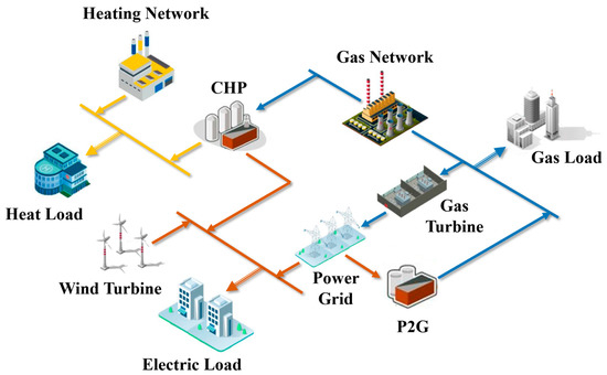
Figure 1.
Structure of electricity–gas–heating system.
2.2. Power Network Model
In order to simplify the power network model and ensure the convexity of the model, this paper uses the DC power flow model to simulate the power network constraints:
In the above, ΩEN is the grid node set; AG, AP2G, and ACHP are node–unit association matrix, node–P2G association matrix, and node–CHP association matrix; PD,t is the node load matrix; B is the imaginary part of the node admittance matrix; θt is the node voltage phase angle vector; and xij are the maximum transmission power and reactance of the line respectively; PG,t is the unit active output vector; PP2G,t is the P2G device consumes active power vector; PCHP,t is the CHP device active input power vector; ad and au are the upper and lower limits of the unit climbing rate constraint; is the balance node phase angle.
2.3. Natural Gas Network Model
The transmission speed of natural gas in pipelines is related to various factors such as pressure and temperature. The natural gas steady-state model ignores the transmission delay of natural gas in the pipeline, and simply equates the pipeline injection gas flow with the outflow gas flow, resulting in an increase in calculation error. This paper uses gas pipeline partial differential equations to describe the dynamic characteristics of natural gas networks:
In the above, , are the gas pressure and gas flow at pipe x at time t, respectively. M1 and M2 are pipe transmission constants and the specific expression of M1, M2 are provided in Appendix B; Equations (2)–(3) are partial differential equations, which are difficult to solve directly. Therefore, they are transformed into algebraic equations by Euler’s finite difference method. The pipe ij is divided into N segments, each segment length is , and the equation is expressed as follows:
In the above, is the time step and is the space step.
There is a delay effect in the transmission of natural gas in the pipeline, and some natural gas is retained in the pipeline, which is called “pipe storage”. After completing a scheduling period, the storage should meet the following constraint:
In the above, ΩGP is a natural gas pipeline collection.
The pressurization station must meet the following constraints:
In the above, , is the pressure before and after boosting; , are the lower and upper limits of the career ratio; is the pipe airflow and is the pipe airflow limit.
Node air pressure and air source output constraints are as follows:
In the above, Ωg and ΩGB are gas source sets and gas node sets, respectively.
Gas tank constraints are as follows:
In the above, Ωs is the collection of gas storage tanks; and are the natural gas input and output of the gas storage tank n at time t, respectively; , are the inflation and deflation efficiency of the gas storage tank n at time t; is the rated gas storage capacity of the gas storage tank n.
The node traffic balancing constraint is as follows:
In the above, Bg, BP2G, BS, BCHP, BGT, and Ag are node–air source correlation matrix, node–P2G correlation matrix, node–gas tank association matrix, node–CHP correlation matrix, node–gas unit association matrix, and node–Pipeline association matrix, respectively. fg,t, fP2G,t, fCHP,t, fGT,t, and fD,t are the gas source output vector, P2G natural gas injection vector, CHP natural gas injection vector, gas unit gas injection vector, and natural gas load vector, respectively.
The dynamic model of the natural gas network can accurately describe the transmission characteristics of natural gas pipelines. The natural gas network is coupled to the power network and the heating network through a gas turbine, CHP. Accurately establishing the natural gas network model can fully explore the potential of EGHS’s energy complementarity.
2.4. Heating Network Model
In the heating network, the water flow is mostly used as the heat medium. The dynamic characteristics of the heat network are mainly reflected in the heat transfer delay and temperature loss. Therefore, in the heating network model, the water flow rate is regarded as constant, and the heating network dynamic characteristics are described as follows:
In the above, and are the water temperature and water flow at the distance from the nozzle x at time t of the k-pipe. is the heat loss factor, and cw is the specific heat capacity of the water. is the density of water and Rk is the radius of the pipe. is the ambient temperature of the k pipe at time t.
Solving Equation (11):
In the above, and are the water inflow and outflow temperatures of the kth pipe at time t. is the time it takes for water to pass through the k-pipe.
The water flow can be regarded as a constant, so the above construction can be converted into the following form:
In the above, Lk is the length of the k pipe and Mk is the water flow of the k pipe.
The electrical and heating output relationship of the CHP unit can be expressed as follows:
In the above, is the unit’s electric-to-heat ratio and is the CHP unit’s heat output. is the water flow. is the water supply temperature. is the return water temperature.
Heat exchange station constraints are as follows:
Heating network node water temperature constraints:
In the above, Ωpipe,out,k and Ωpipe,in,k are the collections of pipes with node k at the outflow point and the inflow point, respectively. Tmix,k is the mixing temperature of node k.
The water temperature of the water supply network and the backwater network meet the following constraints:
In the above, and are the upper and lower limits of the water temperature of the water supply network, respectively. and are the upper and lower limits of the water temperature of the backwater network.
The dynamic model of the heating network can be used to describe the operating characteristics more accurately. The heating energy stored in the pipe can be used as the energy buffer of EGHS, which increases the flexibility of scheduling [19].
2.5. Coupling Device Constraint
Power networks and natural gas networks are coupled with gas turbines and P2G devices and need to meet the following constraints:
In the above, ΩGT, ΩP2G are gas turbines and P2G sets, respectively. PGT,i,t, fGT,i,t are the active power of the gas turbine and the corresponding natural gas consumption at time t. PP2G,j,t, fP2G,j,t are the active power of P2G device and the corresponding natural gas conversion amount at time t. h2,i, h1,i, h0,i, and hP2G,i are coefficients.
In addition, the natural gas network is coupled to the heating network and the power network through the CHP device. The working mode of the CHP is to determine the electrical output through the heat output, and the constraints are as follows:
In the above, ΩCHP is a collection of CHP. HCHP,c,t, PCHP,c,t are CHP heating power and electric power respectively. KCHP,c is the ratio of CHP output power and thermal energy. fCHP,c,t is the natural gas consumption of CHP unit. ηCHP is CHP unit conversion efficiency. HGV is the calorific value of natural gas.
2.6. Objective Function
The objective function is the total operation cost:
In the above, T is the scheduling period. ΩG is the collection of coal-fired units. Ωg is the collection of wind turbines. ΩW is the collection of wind turbines. Ωs is the collection of gas cans. Ωh is the collection of heat sources. PG,i,t is the output of coal-fired unit i at time t. ai, bi, and ci are the unit cost coefficients. fg,j,t is the gas output of the gas source j at time t. ξj is the cost coefficient of purchasing gas. PW,k,max is the upper limit of the wind turbine output. PW,i,t is the output of wind turbine i at time t. δk is the penalty coefficient for discarding wind energy. CS,n,t is the cost coefficient of the gas storage tank. Hh,m,t is the output of heat source m at time t. Ch,m,t is the cost of purchasing heating energy.
The electric–gas–heating system’s daily dispatching model aims at minimizing the operating cost of the system, that is, minimizing the system’s energy supply cost through optimized scheduling.
3. Distributed Optimized Scheduling of EGHS
In order to protect the privacy of each system operation, this paper uses an improved ADMM algorithm to solve the day-ahead scheduling problem. The application of the ADMM algorithm requires that the model is convex, while Equations (5) and (21) are non-convex constraints. Therefore, this paper proposes a convex distributed optimization framework for internal and external co-ordination.
3.1. Outer Layer PCCP Algorithm
The constraint in Equation (5) is processed as follows [20]:
In the above, Equation (27) is a convex constraint. The relaxation of Equation (28) is as follows:
In the above, and are the pressure value and airflow of the pipeline position d + 1 at time t after the k − 1 iteration; is a relaxation variable with a value greater than or equal to 0.
The constraint in Equation (21) is processed as follows:
Since unnecessary gas consumption will increase the cost of energy supply to the system, the constraint in Equation (29) is always tight. In order to keep the relaxation domain tight, the relaxation variables are added to the inner optimization objective function:
In the above, W(k) is the objective function value including the penalty function obtained by the kth optimization; ρ(k) is the penalty factor for the kth iteration of the outer PCCP; Ωd is the set of relaxation variables.
The convergence conditions of PCCP are as follows:
In the above, ε1 and ε2 are convergence determination parameters; δ is the relaxation variable matrix; If the convergence conditions are not met, the penalty factor is updated as follows:
In the above, ρmax is the maximum penalty factor; vc is the dynamic adjustment coefficient.
3.2. Inner Layer ADMM-FE Algorithm
Generally, ADMM is only used to solve two-operator problems. The electricity–gas–heating system model constructed in this paper is a three-operator problem. If the ADMM is directly extended by the three operators, the calculation result does not necessarily converge. The electricity–gas–heating system optimization problem is as follows:
In the above, x, y, and z are separable three operators. A, B, and C are the constraint coefficient vectors related to the grid, gas network, and heat grid, respectively. D is the parameter vector of the correlation equation.
Augmented Lagrangian function:
In the above, is an augmented Lagrangian function that introduces Lagrangian multiplier λ and penalty factor η.
The standard ADMM iteration format is as follows:
The above formula is a standard ADMM iterative format, and its convergence is guaranteed, but yk+1 and zk+1 are updated synchronously, and distributed computing is not implemented. In order to achieve fully distributed computing, ADMM is directly promoted as follow:
Comparing Equation (35) with Equation (36), Equation (35) uses (Axk+1, Byk, Czk,λk) to update yk+1, but Equation (29) uses (Axk+1, Byk, Czk+1, λk) to update yk+1. The equal status of y and z is destroyed, resulting in the algorithm may not converge. Therefore, modify the iteration format as follows:
The above formula updates yk+1 and zk+1 with the same information, guarantees the equal and parallel processing of y and z, and adds regular items when updating y and z. The meaning is to add a self-constraining mechanism to the variable to correct the variables. The improved ADMM algorithm guarantees the convergence of the algorithm by forcing equal updates of the variables. The improved algorithm is ADMM-FE.
3.3. PCCP-ADMM-FE Algorithm Steps
Based on the above algorithms, a convex distributed optimization framework for internal and external co-ordination is established in this paper. The specific steps are as follows:
(1) Initialize the parameters of the EGHS system, ignore Equation (28), and use the second-order cone program model to obtain a good initial iteration point. Initialize PCCP parameters and enter the inner layer calculation.
(2) Relax the equality constraint to the objective function, then yield an augmented Lagrange function:
In the above, XP2G, XG2P, and XCHP are the P2G, G2P, and CHP variables in the power grid, respectively. YP2G, YG2P, and YCHP are P2G, G2P, and CHP variables in the gas network, respectively. ZP2G is the CHP variable in the heating network.
The iteration format of ADMM-FE is as follows:
In the above, Ce, Cg, and Ch are the power grid, gas network, and heat grid costs separated in the objective function, respectively. λxy,k is the Lagrange multiplier of the grid and gas network coupling variables. λzy,k is the Lagrange multiplier of the coupled variable of the heating network and the gas network. λxz,k is the Lagrange multiplier of the coupled variable of the grid and the heating network.
In the above, ρ, τ, and β are penalty parameters. k1, k2, k3 are the conversion coefficients of the coupling variables of the CHP equipment between the grid, the gas network, and the heating network. λP2G,k and λG2P,k are the Lagrange multipliers of the grid and gas network P2G coupling equipment and G2P coupling equipment respectively. λCHPxy,k, λCHPzy,k, and λCHPxz,k are Lagrange multipliers of CHP coupling devices.
(3) The inner ADMM-FE convergence decision is as follows:
In the above, εx, εy, and εz are the absolute values of the maximum difference between the boundary variables of each subsystem after the kth iteration. εk is the maximum of , , and .
When the difference between the boundary variables calculated by the kth and the k+1th time is less than a certain value, and the rate of change of the objective function values between the continuous two-time calculation is less than a certain value, the algorithm is considered to be convergent. The convergence is determined as follows:
In the above, a and b are constants used to determine whether or not to converge.
(4) Outer layer ADMM-FE convergence decision: Judge according to Equations (31) and (32).
4. Case Studies
Based on the proposed EGHS scheduling model and solving algorithm, an example is established for analysis. The Example System 1 is as shown in Appendix A Figure A1. It consists of a modified IEEE39 node network, a Belgian 20-node natural gas network, and an 8-node heating network. The Example System 2 is as shown in Appendix A Figure A2. In this process, the heat network of Example System 1 is changed to a 20-node heat network. All tests are performed on a computer with four processors running at 2.30 GHz with 64 GB of memory. Programs are coded using MATLAB R2018a and GAMS.
4.1. Example Description
The power network is a modified IEEE39 node power system. There are 46 transmission lines in the system. The original system contains 10 coal-fired units. Set G1, G7, and G8 as gas units, which are respectively connected to the 4, 10, and 12 nodes of the natural gas network. Set G4 and G5 as the wind turbine connected to the 33 and 34 nodes. In order to maximize wind power, the P2G input is connected to nodes 33 and 34. The system load is set to 85% of the original load, and the cost of wind abandonment is $50/(MW.h). The remaining generator set parameters are recorded in Appendix A Table A1 and Table A2.
The natural gas network is a modified Belgian 20-node natural gas network. There are 24 gas pipelines in the system. The system consists of two gas sources, three pressurization stations, and four gas storages. P2G output is connected at 13 and 14. The system load is 20% of the original load, and the gas source energy supply cost is $ 0.3/m3. The remaining parameters are recorded in Appendix A Table A3.
In the example of System 1, the heating network is an 8-node heating network. The system contains 14 water pipes and 2 heat sources. Nodes (1~4) and nodes (5~8) respectively form independent systems, and the two systems are not directly connected. CHP is connected to 1 node and 5 nodes respectively. Heating network parameters are recorded in Appendix A Figure A3.
In the example of System 2, the heating network is a 20-node heating network: the system has a total of 19 water pipelines; CHP is connected at 1 and 8 nodes respectively.
The schematic diagram of the constructed EGHS is shown in Appendix A Figure A1 and Figure A2, respectively. Set the algorithm parameter values: ρ = 0.65, τ = 2, a = 0.001, b = 0.0001; Set the CHP thermoelectric ratio to 0.8, then k1 = 1.8, k2 = 2.25, k3 = 1.25.
4.2. Algorithm Performance Comparision
4.2.1. Comparison of PCCP-ADMM-FE and Centralized Algorithm Results
In order to compare the optimization results and convergence speed of the proposed algorithm with the centralized algorithm, the optimization results of the example system under the ADMM-FE algorithm are compared with the centralized optimization results. Set ρ0 = 10−3, the optimization results are shown in Table 1.

Table 1.
Results comparison of centralized optimization and alternating direction method of multipliers (ADMM)-FE (forced equality) algorithms.
The analysis of Table 1 is as follows:
- (1)
- Under the constraint of convergence accuracy a = 0.001, b = 0.0001, ε1 = 0.001, ε2 = 0.001, both the proposed algorithm and the centralized algorithm can get a convergent optimal solution. Compared with the results of centralized optimization, the error of the calculation result of the proposed algorithm is less than 10−3. Optimization results verify the accuracy and effectiveness of the algorithm;
- (2)
- The ADMM-FE calculation time is longer than the centralized calculation time, but the information privacy of each subsystem is guaranteed. From the scale of formulating the daily dispatch plan, it is acceptable to sacrifice a small amount of calculation speed in exchange for the decentralized autonomy of each subsystem.
4.2.2. Convergence Comparison between ADMM-FE and Directly Generalized ADMM
Taking the iterative process of obtaining the initial point as an example, the convergence of the ADMM-FE algorithm and the directly generalized ADMM algorithm is compared and analyzed. According to the algorithm parameter settings, under the constraints of a = 0.001 and b = 0.0001, the maximum imbalance amount εk in the optimization process is shown in Figure 2. The ratio of the target difference between the two iterations is shown in Figure 3.
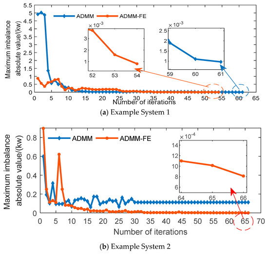
Figure 2.
The absolute maximum value of the unbalanced amount.
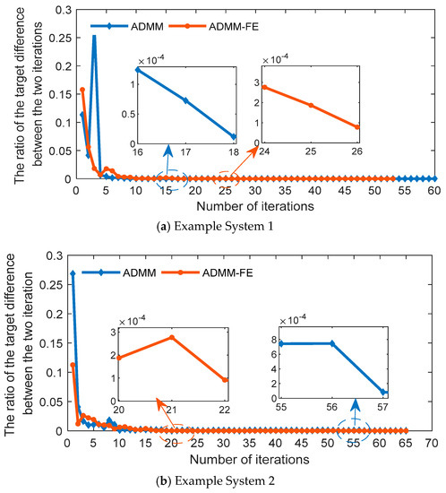
Figure 3.
Unbalanced amount of objective function.
As can be seen from Figure 2 and Figure 3, in Example System 1, both ADMM and ADMM-FE can obtain convergence solutions, but in Example System 2, when the 66th iteration of ADMM-FE is completed, the boundary variable imbalance has reached the convergence condition, but the boundary variables cannot converge in ADMM. It can be seen that in solving the 3-Block problem, the directly popularized ADMM does not necessarily converge, but the ADMM-FE algorithm proposed in this paper has good convergence characteristics and convergence speed.
4.3. Operation Result Analysis
4.3.1. Model Optimization Run Results
We take Example System 1 as an example and analyzed the model optimization results. PCCP-ADMM-FE was used to optimize Example System 1. The calculation example sets the scheduling period T = 24 h, and the simulation step size was 1 h.
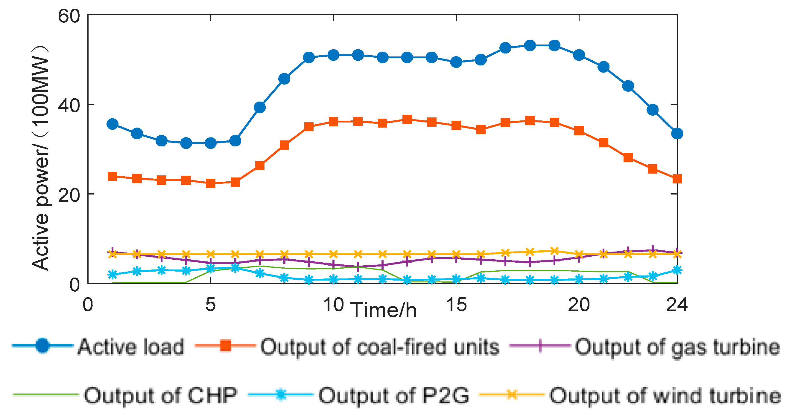
Figure 4, Figure 5 and Figure 6 respectively show the power network conditions, gas network conditions, and heating network conditions in the optimization results.
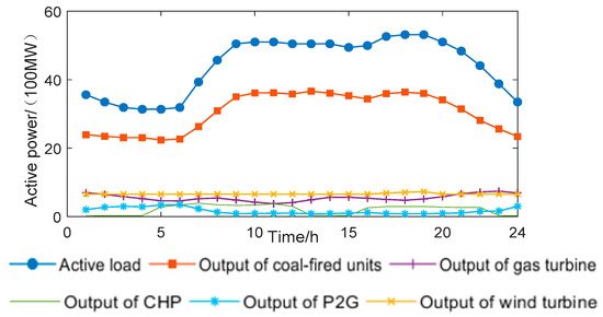
Figure 4.
Power network optimized operation data.
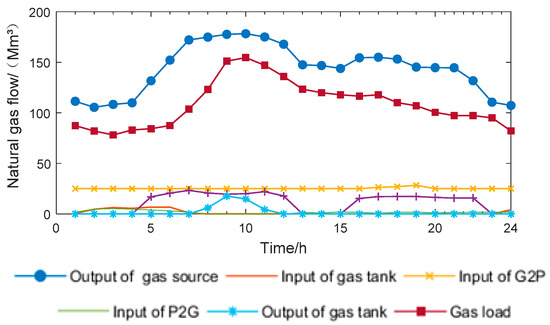
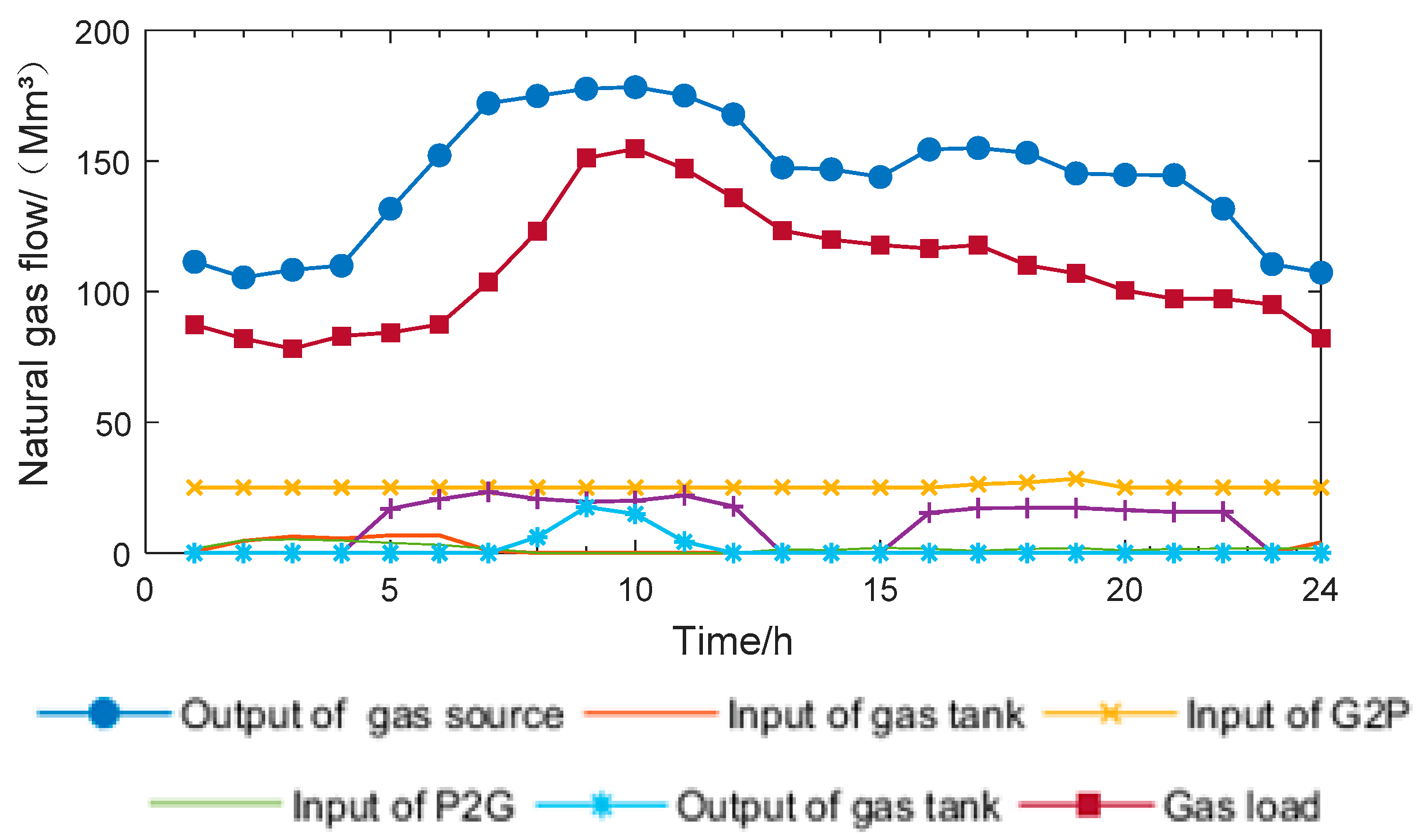
Figure 5.
Gas network optimized operation data.

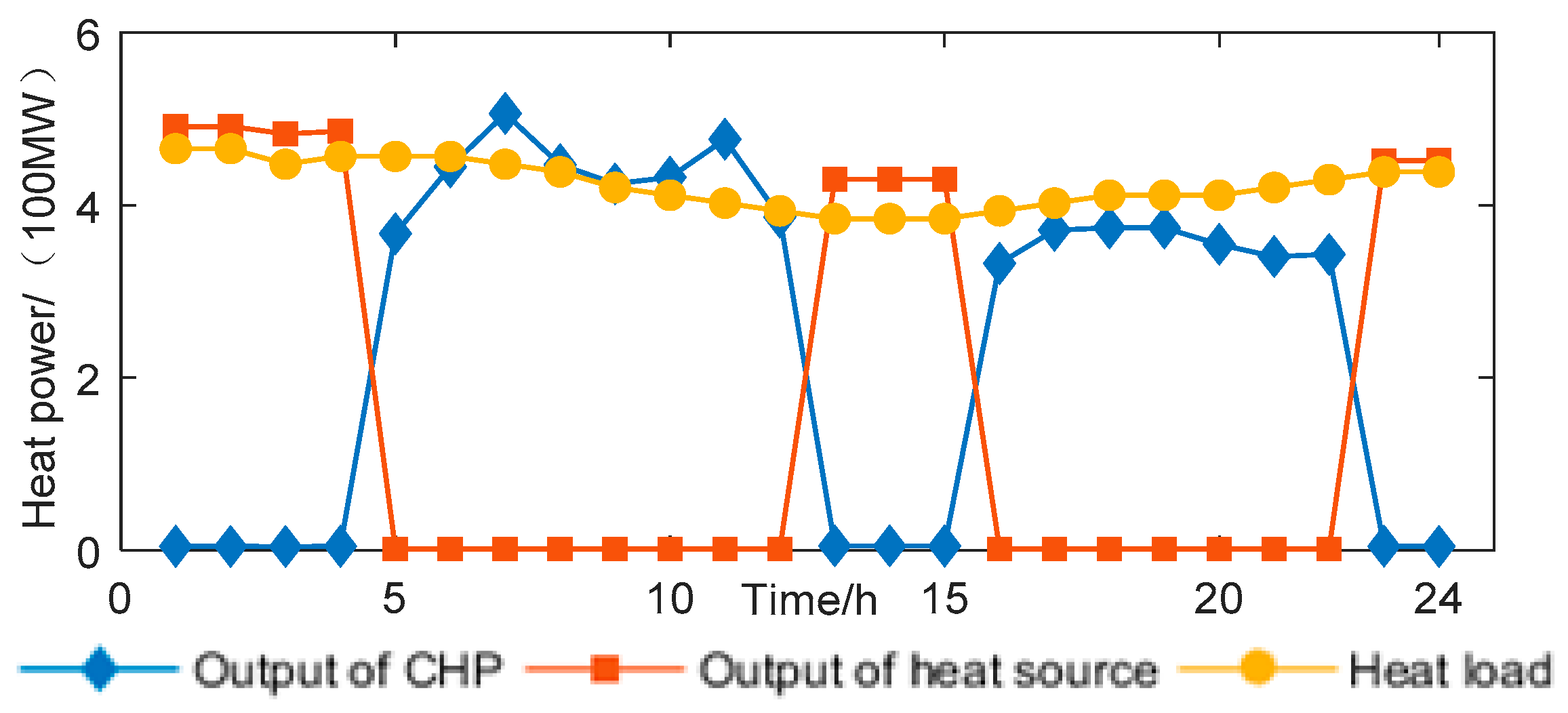
Figure 6.
Heating network optimized operation data.
It can be seen from Figure 4 that in the power network, in the early morning hours, the power load is low, and the wind turbine output is high. At this time, the power of the P2G device can convert the wind power into natural gas storage to absorb the wind power. After 7 o’clock, the daytime work starts, the electric load increases, the grid can absorb all the wind power, so the power of the P2G device drops to 0. In the evening, the power load reaches a peak, and the output of the coal-fired unit reaches the upper limit. At this time, the gas turbine output with higher output cost is called to maintain the power balance. At other times, the coal-fired unit’s own output can meet the load demand, so the gas turbine output has been maintained at the lowest level. Therefore, the gas turbine output will maintain the lowest value during the period except for fluctuations from 17 to 19 h. The electrical output of the CHP device is determined by the thermal output. Therefore, in addition to the CHP heating for the demand of heating networks during 6~12 h and 16~22 h, the CHP output grid power is zero.
It can be seen from Figure 5 that in the gas network, in the early morning hours, the gas load and the gas consumption of the gas turbine are low, and the grid inputs high natural gas for the wind power converted by P2G, so the gas tank input is high with 0 output, and the surplus natural gas is stored in the gas storage tank used as a slow storage energy. During the daytime working hours, as the air load increases and the heating-network-demand CHP increases, the gas tank input decreases and the output increases. At 9 h, the gas load peaks and the gas tank output peaks.
It can be seen from Figure 6 that in the heating network, in the early morning hours, the external heat source energy supply cost is lower than the CHP and is at a low price. Therefore, the heat load is satisfied by the external heat source, and the energy supply is greater than the heat load, so the excess heat is used as the heat storage energy. During the daytime working hours, the external heat source energy supply cost is higher than the CHP, so the heat load is transferred to be satisfied by the CHP energy supply. The CHP energy supply is greater than the heat load in some periods, so the excess CHP energy supply is used as the heat network energy storage to eliminate the storage from the gas network during nighttime. From 16 o’clock to 21 o’clock, the heat storage and external heat sources meet the heat load requirements.
4.3.2. The Effect of Heating Network Dynamic Properties on Optimal Operation
In order to explore the influence of the dynamic characteristics of the heating network on the overall optimization operation of the system, this paper draws the correlation between CHP output, external heat source energy supply and heat load under the condition of neglecting the dynamic characteristics of the heating network and considering the dynamic characteristics of the heating network. Ignore the dynamic characteristics of the heating network, that is, ignore Equations (11), (12), (13), and replace them by the following Equation (45) instead:
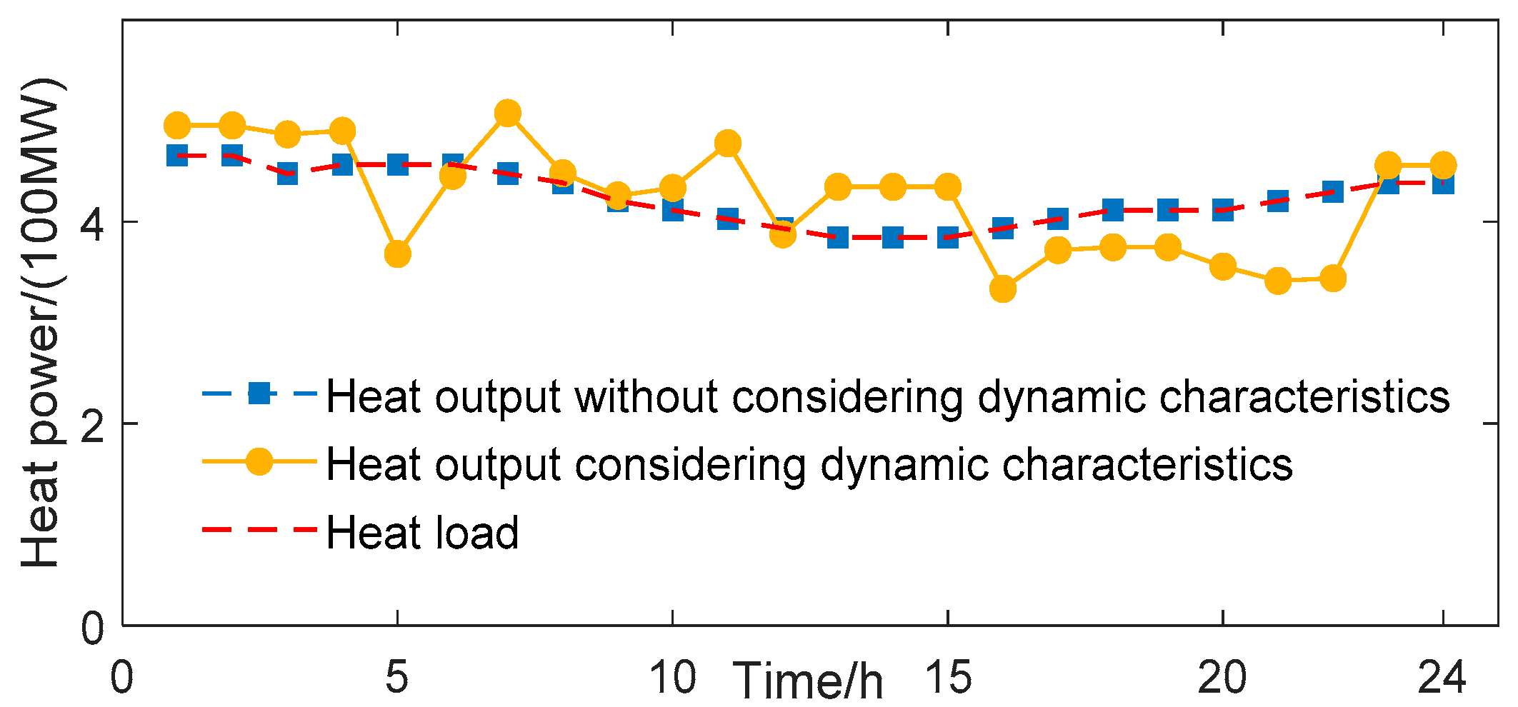
As shown in Figure 7, under the condition of neglecting the dynamic characteristics of the heating network, the CHP output and the external heat source output are constrained by the heat load, and the output and load are coincident. After considering the dynamic characteristics of the heating network, the CHP output and the heat source output are no longer subject to the heat load. During 5~6 h, 16~22 h, the heat load is higher than the heat output, and the heat load is satisfied by CHP, external heat source and heat storage. In the rest of the time, the heat output is higher than the heat load, so the excess heat energy is stored in the heat network as the heat storage energy.
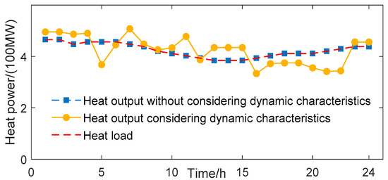
Figure 7.
Relationships between heat output and load.
It can be seen that after considering the dynamic characteristics of the heating network, it can be used as energy storage to decouple the heat source output and heat load to a certain extent. When the heating cost is low or the renewable energy needs to be consumed, the heating network performs energy storage, and the energy storage is called during the peak of heating, which improves the flexibility of system scheduling.
5. Conclusions
In this paper, a day-ahead scheduling model of EGHS considering the dynamic characteristics of the networks is established, and a convex distributed optimization algorithm for inner and outer layer co-ordination based on the ADMM-FE algorithm is proposed. Simulation analysis verifies that the algorithm in this paper can effectively obtain a convergent optimal solution in the three-region distributed optimization problem of the EGHS under the condition of protecting the privacy of the information of each subsystem.
In reality, each subsystem may have different optimization objectives besides cost requirements, and there may be conflicts between different optimization targets. Therefore, in the follow-up work, the game between the power system, natural gas system, and heating system in an open market environment and the multi-objective dispersion optimization problem of EGHS will be the main research direction. In addition, the calculation speed of the ADMM-FE algorithm is slower than the centralized algorithm. In the next work, the author will further study how to improve the calculation speed of the ADMM-FE algorithm.
Author Contributions
Methodology, H.Z.; investigation, W.W.; data curation, Z.L.; formal analysis, H.Z.; writing—original draft preparation, H.Z.; writing—review and editing, H.Z.; supervision, T.Y. All authors have read and agreed to the published version of the manuscript.
Funding
This research was funded by the National Natural Science Foundation of China (Grant. 51477055&51777078).
Acknowledgments
The authors gratefully acknowledge the support of the National Natural Science Foundation of China.
Conflicts of Interest
The authors declare no conflict of interest.
Appendix A
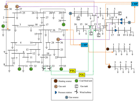
Figure A1.
The structure of Example System 1.
Figure A1.
The structure of Example System 1.
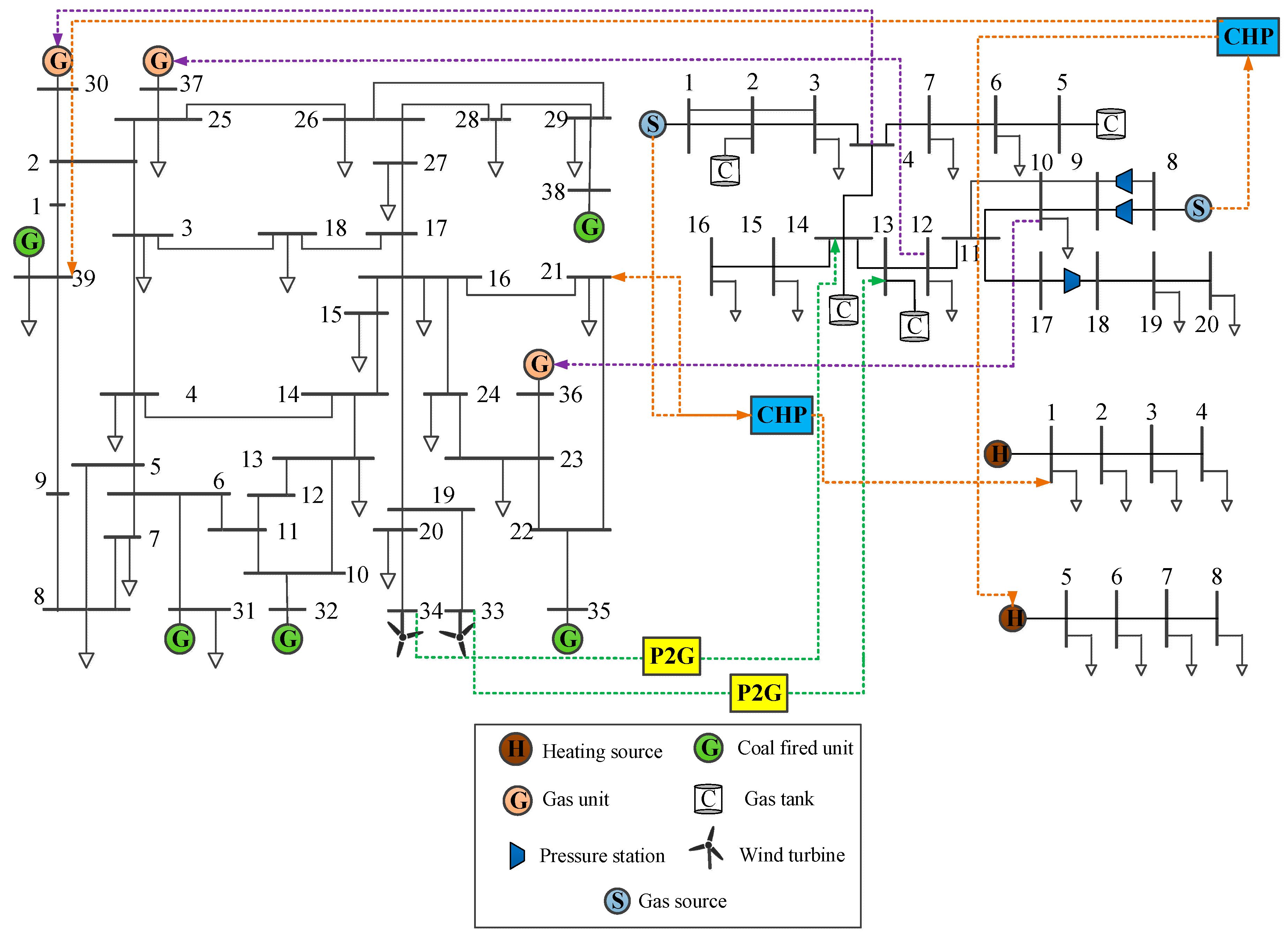
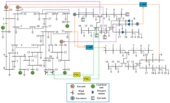
Figure A2.
The structure of Example System 2.
Figure A2.
The structure of Example System 2.
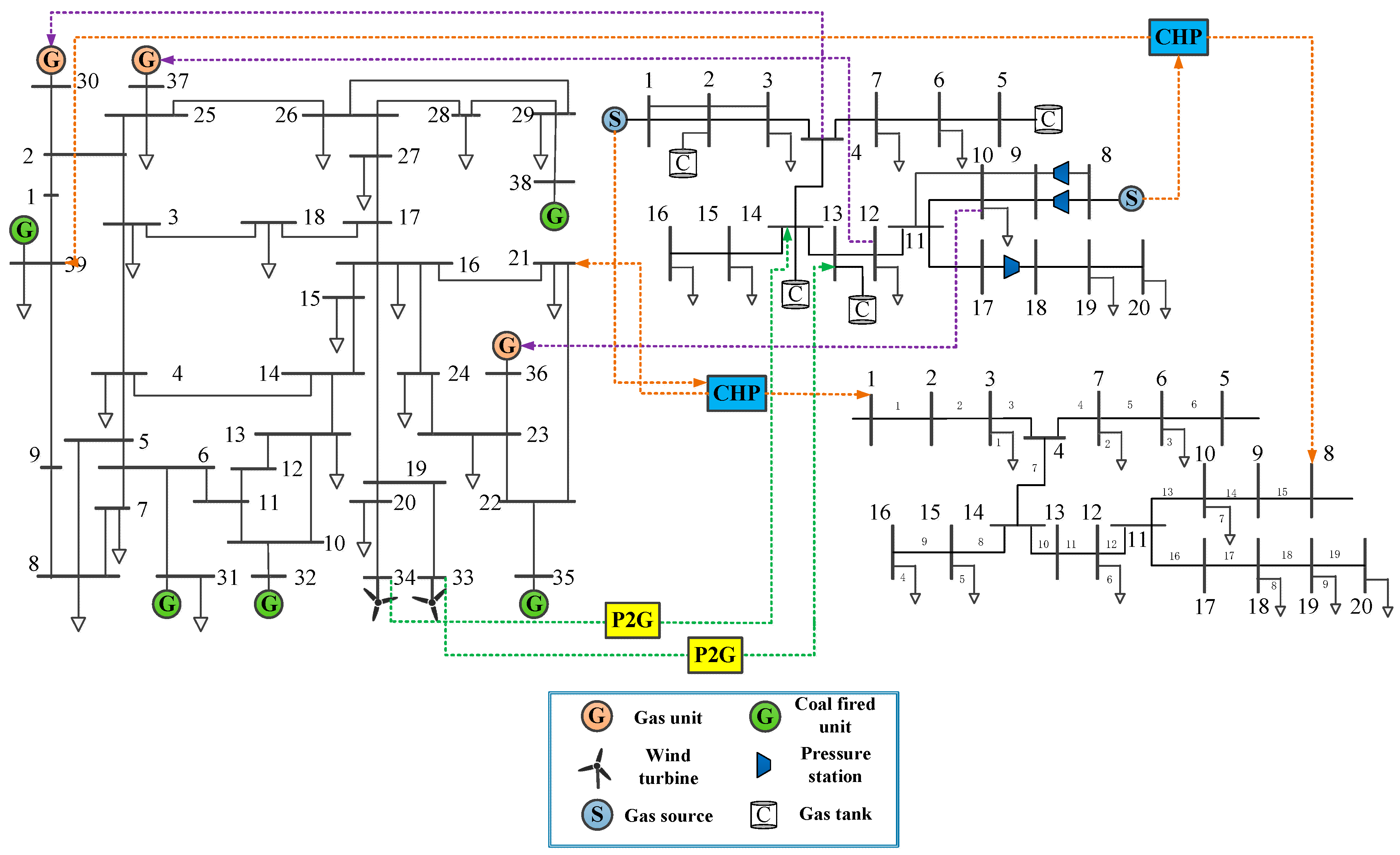
Table A1.
Parameters of gas units.
Table A1.
Parameters of gas units.
| Gas Unit | Electric Network Node | Gas Network Node | Pmax/MW |
|---|---|---|---|
| G1 | 30 | 4 | 520 |
| G7 | 36 | 10 | 290 |
| G8 | 37 | 12 | 280 |
Table A2.
Parameters of coal fired units.
Table A2.
Parameters of coal fired units.
| Coal Fired Unit | Cost Coefficient | Pmax/MW | ||
|---|---|---|---|---|
| a | b | c | ||
| G2 | 0.700 | 27 | 0 | 646 |
| G3 | 0.682 | 22 | 0 | 725 |
| G6 | 0.425 | 25 | 0 | 687 |
| G9 | 0.458 | 26 | 0 | 865 |
| G10 | 0.890 | 25 | 0 | 1100 |
Table A3.
Parameters of sources.
Table A3.
Parameters of sources.
| Gas Source | Gas Network Node | Upper Limit of Capacity/m3 | Lower Limit of Capacity/m3 | Upper Limit of Output/(m3/s) | Lower Limit of Output/(m3/s) |
|---|---|---|---|---|---|
| S1 | 1 | — | — | 150.52 | 10.27 |
| S2 | 8 | — | — | 150.24 | 11.97 |
| C1 | 2 | 175.00 | 29.17 | 29.17 | 29.17 |
| C2 | 5 | 100.00 | 16.67 | 16.67 | 16.67 |
| C3 | 13 | 25.00 | 4.17 | 4.17 | 4.17 |
| C4 | 14 | 117.22 | 19.54 | 19.54 | 19.54 |
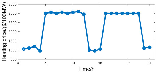
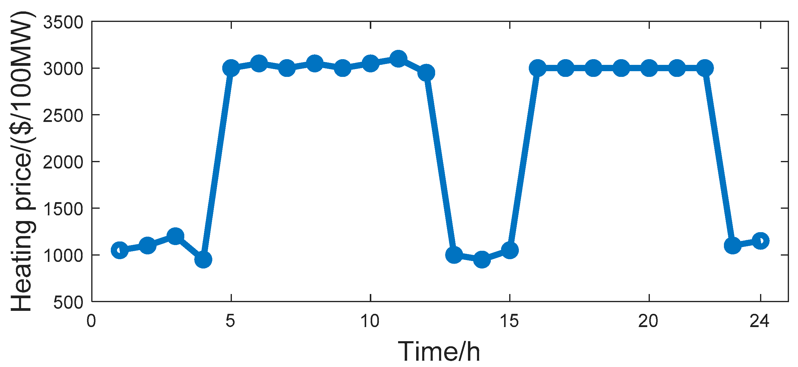
Figure A3.
Heating price.
Figure A3.
Heating price.
Appendix B
In Equations (2) and (3), M1 and M2 are constants depending on the parameters of the pipelines. The specific formulations are as follows (SI Units):
In the above, where f and D denote the friction factor and diameter of the gas pipeline. T means the average temperature of natural gas in the pipeline. Ps and Ts are the pressure and temperature under standard conditions (101325 Pa, 298 K). Rg is the gas constant for natural gas which equals the standard gas constant divided by the molar mass of natural gas.
References
- Aluisio, B.; Dicorato, M.; Forte, G.; Trovato, M. An optimization procedure for microgrid day-ahead operation in the presence of CHP facilities. Sustain. Energy Grids Netw. 2017, 11, 34–45. [Google Scholar] [CrossRef]
- Rehman, M.H.G.; Reisslein, M.G.; Rachedi, A.; Erol-Kantarci, M.G.; Radenkovic, M.G. Integrating renewable energy resources into the smart grid: Recent developments in information and communication technologies. IEEE Trans. Ind. Inf. 2018, 14, 2814–2825. [Google Scholar] [CrossRef]
- Fathi, M.; Bevrani, H. Statistical cooperative power dispatching in interconnected microgrids. IEEE Trans. Sustain. Energy 2013, 4, 586–593. [Google Scholar] [CrossRef]
- Wang, J.; Zhong, H.; Xia, Q.; Kang, C.; Du, E. Optimal joint-dispatch of energy and reserve for CCHP-based microgrids. IET Gener. Transm. Distrib. 2017, 11, 785–794. [Google Scholar] [CrossRef]
- Wen, Y.; Qu, X.; Li, W.; Liu, X.; Ye, X. Synergistic Operation of Electricity and Natural Gas Networks via ADMM. IEEE Trans. Smart Grid 2018, 9, 4555–4565. [Google Scholar] [CrossRef]
- Chen, J.; Zhang, W.; Zhang, Y.; Bao, G. Day-Ahead Scheduling of Distribution Level Integrated Electricity and Natural Gas System Based on Fast-ADMM With Restart Algorithm. IEEE Access 2018, 6, 17557–17569. [Google Scholar] [CrossRef]
- Martinez-Mares, A.; Fuerte-Esquivel, C.R. A Unified Gas and Power Flow Analysis in Natural Gas and Electricity Coupled Networks. IEEE Trans. Power Syst. 2012, 4, 2156–2166. [Google Scholar] [CrossRef]
- He, C.; Wu, L.; Liu, T.; Shahidehpour, M. Robust Co-Optimization Scheduling of Electricity and Natural Gas Systems via ADMM. IEEE Trans. Sustain. Energy 2017, 8, 658–670. [Google Scholar] [CrossRef]
- Bao, Y.; Wu, M.; Zhou, X.; Tang, X. Piecewise Linear Approximation of Gas Flow Function for the Optimization of Integrated Electricity and Natural Gas System. IEEE Access 2019, 7, 91819–91826. [Google Scholar] [CrossRef]
- Manshadi, S.D.; Khodayar, M.E. Co-ordinated Operation of Electricity and Natural Gas Systems: A Convex Relaxation Approach. IEEE Trans. Smart Grid 2019, 10, 3342–3354. [Google Scholar] [CrossRef]
- Ge, H.; Liu, F.; Chen, H.; Zhang, C. Co-Ordinated Optimization of District Electricity and Heating System Based on Genetic Algorithm. In Proceedings of the 2016 IEEE PES Asia-Pacific Power and Energy Engineering Conference (APPEEC), Xi’an, China, 25–28 October 2016; pp. 1543–1547. [Google Scholar]
- Yang, J.; Zhang, N.; Kang, C.; Xia, Q. Effect of Natural Gas Flow Dynamics in Robust Generation Scheduling Under Wind Uncertainty. IEEE Trans. Power Syst. 2018, 33, 2087–2097. [Google Scholar] [CrossRef]
- Shao, C.; Wang, X.; Wang, X.; Du, C.; Wang, B. Hierarchical Charge Control of Large Populations of EVs. IEEE Trans. Smart Grid 2016, 7, 1147–1155. [Google Scholar]
- Zhang, H.; Li, Y.; Gao, D.W.; Zhou, J. Distributed Optimal Energy Management for Energy Internet. IEEE Trans. Ind. Inform. 2017, 13, 3081–3097. [Google Scholar] [CrossRef]
- Dos Santos, T.N.; Diniz, A.; Borges, C.T. A New Nested Benders Decomposition Strategy for Parallel Processing Applied to the Hydrothermal Scheduling Problem. In Proceedings of the 2017 IEEE Power & Energy Society General Meeting, Chicago, IL, USA, 16–20 July 2017; Volume 1. [Google Scholar]
- Zhang, H.; Moura, S.J.; Hu, Z.; Qi, W.; Song, Y. Joint PEV Charging Network and Distributed PV Generation Planning Based on Accelerated Generalized Benders Decomposition. IEEE Trans. Transp. Electrif. 2018, 4, 789–803. [Google Scholar] [CrossRef]
- Li, Z.; Wu, W.; Zhang, B.; Wang, B. Decentralized Multi-Area Dynamic Economic Dispatch Using Modified Generalized Benders Decomposition. IEEE Trans. Power Syst. 2016, 31, 526–538. [Google Scholar] [CrossRef]
- Chen, C.H.; He, B.S.; Ye, Y.Y. The direct extension of ADMM for multi-block conver min-imization problems is not necessarily convergent. Math. Program. 2016, 155, 57–79. [Google Scholar] [CrossRef]
- Li, Z.; Wu, W.; Shahidehpour, M. Combined heat and power dispatch considering pipeline energy storage of district heating network. IEEE Trans. Sustain. Energy 2016, 7, 12–22. [Google Scholar] [CrossRef]
- Wang, C.; Wei, W.; Wang, J.; Bai, L.; Liang, Y.; Bi, T. Convex Optimization Based Distributed Optimal Gas-Power Flow Calculation. IEEE Trans. Sustain. Energy 2018, 9, 1145–1156. [Google Scholar] [CrossRef]


© 2020 by the authors. Licensee MDPI, Basel, Switzerland. This article is an open access article distributed under the terms and conditions of the Creative Commons Attribution (CC BY) license (http://creativecommons.org/licenses/by/4.0/).