1. Introduction
With the further advancement of the industrialization reform of the energy industry, the energy internet has received increasing attention and research. Integrated energy systems (IES) that include gas units, gas to power (P2G) equipment, and combined heat and power (CHP) equipment break the barriers to exchange between different forms of energy. Therefore, the integrated energy system can fully tap the potential of each energy to complement each other efficiently, and meet various requirements of economic and environmental protection [
1,
2,
3,
4]. In addition, in the open electricity market environment, the electricity supplier, gas supplier, and heating supplier in the electric heat interconnection system generally belong to different suppliers, it is important to ensure the privacy of the information in the co-ordinated operation, so data needs to be protected [
5,
6].
Many research works are reported, focusing on optimization technologies of IES which combine two types of energy flow. Some researchers established an electricity–gas system considering the influence of temperature, and convexified the power grid [
7]. Finally, the optimal power flow was studied on this model. A robust co-optimization scheduling model was proposed to study the co-ordinated optimal operation of electricity–gas systems, and the optimization problem of the model was solved by the alternating direction method of multipliers [
8]. The research proposed the piecewise linear approximation methods to solve the non-convex and non-linear Weymouth equation in gas networks [
9]. However, the above studies are mostly based on a single electricity–gas system or electricity–heating system. There are few studies that concentrate on the electricity–gas–heating system and most are lacking consideration of network dynamic characteristics. Based on this, this paper builds a day-ahead scheduling optimization model of the electricity–gas–heating system (EGHS), considering the dynamic characteristics of the network in order to tap the potential of complementary advantages between different energy flows.
On the other hand, in the existing research, the optimization methods of the IES system mostly adopt the centralized optimization method. A convex relaxation approach was proposed to achieve the co-ordinated operation of electricity and natural gas systems [
10]. Some researchers used a genetic algorithm to achieve the co-ordinated optimization of the district electricity and heating system [
11]. However, the centralized solution used in the above research requires an upper-level co-ordination center to collect the operating information of each subsystem to solve the optimal strategy, which ignores the actual needs of each subsystem to protect its privacy. Distributed computing methods can solve this problem. The distributed algorithm mainly includes the alternating direction multiplier method [
12,
13,
14] and the Benders decomposition algorithm [
15,
16,
17]. This kind of distributed algorithm is only for the 2-Block problem, meaning it is only used to solve the electricity–gas system or the electricity–heating system. The EGHS contains three subsystems, so it belongs to the 3-Block problem in distributed optimization. Therefore, conventional distributed algorithms cannot ensure the convergence of calculation results [
18].
Aiming at the above problems, this paper builds a day-ahead scheduling model of the EGHS considering the dynamic characteristics of the network, then uses inner and outer algorithms to solve the model. The outer penalty convex–concave procedure (PCCP) is responsible for the model convexification and the inner alternating direction method of multipliers (ADMM)-FE (forced equality) gets a convergent solution.
The rest of the paper is structured as follows:
Section 2 establishes a day-ahead scheduling model of the EGHS.
Section 3 introduces the PCCP-ADMM-FE algorithm for the day-ahead scheduling. Numeral testing results are provided in
Section 4. Finally, conclusions are summarized in
Section 5.
2. Day-ahead Scheduling Model for EGHS
2.1. The Structure of EGHS
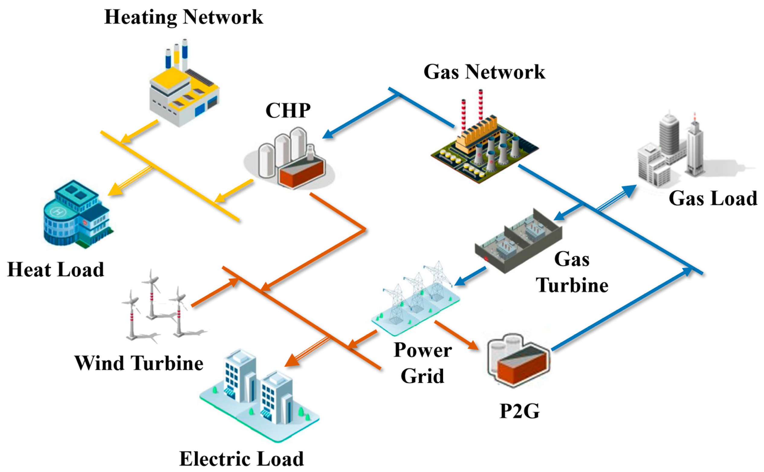
The EGHS studied in this paper consists of a power network, a natural gas network, and a heating network. Among them, the grid converts electric energy to natural gas through P2G equipment. The gas network converts natural gas to heat energy and electric energy through CHP equipment, and the gas network also converts natural gas to electric energy through the gas turbine. The coupling relationship between the systems is shown in
Figure 1.
2.2. Power Network Model
In order to simplify the power network model and ensure the convexity of the model, this paper uses the DC power flow model to simulate the power network constraints:
In the above, ΩEN is the grid node set; AG, AP2G, and ACHP are node–unit association matrix, node–P2G association matrix, and node–CHP association matrix; PD,t is the node load matrix; B is the imaginary part of the node admittance matrix; θt is the node voltage phase angle vector; and xij are the maximum transmission power and reactance of the line respectively; PG,t is the unit active output vector; PP2G,t is the P2G device consumes active power vector; PCHP,t is the CHP device active input power vector; ad and au are the upper and lower limits of the unit climbing rate constraint; is the balance node phase angle.
2.3. Natural Gas Network Model
The transmission speed of natural gas in pipelines is related to various factors such as pressure and temperature. The natural gas steady-state model ignores the transmission delay of natural gas in the pipeline, and simply equates the pipeline injection gas flow with the outflow gas flow, resulting in an increase in calculation error. This paper uses gas pipeline partial differential equations to describe the dynamic characteristics of natural gas networks:
In the above,
,
are the gas pressure and gas flow at pipe
x at time
t, respectively. M
1 and M
2 are pipe transmission constants and the specific expression of M1, M2 are provided in
Appendix B; Equations (2)–(3) are partial differential equations, which are difficult to solve directly. Therefore, they are transformed into algebraic equations by Euler’s finite difference method. The pipe
ij is divided into N segments, each segment length is
, and the equation is expressed as follows:
In the above, is the time step and is the space step.
There is a delay effect in the transmission of natural gas in the pipeline, and some natural gas is retained in the pipeline, which is called “pipe storage”. After completing a scheduling period, the storage should meet the following constraint:
In the above, ΩGP is a natural gas pipeline collection.
The pressurization station must meet the following constraints:
In the above, , is the pressure before and after boosting; , are the lower and upper limits of the career ratio; is the pipe airflow and is the pipe airflow limit.
Node air pressure and air source output constraints are as follows:
In the above, Ωg and ΩGB are gas source sets and gas node sets, respectively.
Gas tank constraints are as follows:
In the above, Ωs is the collection of gas storage tanks; and are the natural gas input and output of the gas storage tank n at time t, respectively; , are the inflation and deflation efficiency of the gas storage tank n at time t; is the rated gas storage capacity of the gas storage tank n.
The node traffic balancing constraint is as follows:
In the above, Bg, BP2G, BS, BCHP, BGT, and Ag are node–air source correlation matrix, node–P2G correlation matrix, node–gas tank association matrix, node–CHP correlation matrix, node–gas unit association matrix, and node–Pipeline association matrix, respectively. fg,t, fP2G,t, fCHP,t, fGT,t, and fD,t are the gas source output vector, P2G natural gas injection vector, CHP natural gas injection vector, gas unit gas injection vector, and natural gas load vector, respectively.
The dynamic model of the natural gas network can accurately describe the transmission characteristics of natural gas pipelines. The natural gas network is coupled to the power network and the heating network through a gas turbine, CHP. Accurately establishing the natural gas network model can fully explore the potential of EGHS’s energy complementarity.
2.4. Heating Network Model
In the heating network, the water flow is mostly used as the heat medium. The dynamic characteristics of the heat network are mainly reflected in the heat transfer delay and temperature loss. Therefore, in the heating network model, the water flow rate is regarded as constant, and the heating network dynamic characteristics are described as follows:
In the above, and are the water temperature and water flow at the distance from the nozzle x at time t of the k-pipe. is the heat loss factor, and cw is the specific heat capacity of the water. is the density of water and Rk is the radius of the pipe. is the ambient temperature of the k pipe at time t.
In the above, and are the water inflow and outflow temperatures of the kth pipe at time t. is the time it takes for water to pass through the k-pipe.
The water flow can be regarded as a constant, so the above construction can be converted into the following form:
In the above, Lk is the length of the k pipe and Mk is the water flow of the k pipe.
The electrical and heating output relationship of the CHP unit can be expressed as follows:
In the above, is the unit’s electric-to-heat ratio and is the CHP unit’s heat output. is the water flow. is the water supply temperature. is the return water temperature.
Heat exchange station constraints are as follows:
Heating network node water temperature constraints:
In the above, Ωpipe,out,k and Ωpipe,in,k are the collections of pipes with node k at the outflow point and the inflow point, respectively. Tmix,k is the mixing temperature of node k.
The water temperature of the water supply network and the backwater network meet the following constraints:
In the above, and are the upper and lower limits of the water temperature of the water supply network, respectively. and are the upper and lower limits of the water temperature of the backwater network.
The dynamic model of the heating network can be used to describe the operating characteristics more accurately. The heating energy stored in the pipe can be used as the energy buffer of EGHS, which increases the flexibility of scheduling [
19].
2.5. Coupling Device Constraint
Power networks and natural gas networks are coupled with gas turbines and P2G devices and need to meet the following constraints:
In the above, ΩGT, ΩP2G are gas turbines and P2G sets, respectively. PGT,i,t, fGT,i,t are the active power of the gas turbine and the corresponding natural gas consumption at time t. PP2G,j,t, fP2G,j,t are the active power of P2G device and the corresponding natural gas conversion amount at time t. h2,i, h1,i, h0,i, and hP2G,i are coefficients.
In addition, the natural gas network is coupled to the heating network and the power network through the CHP device. The working mode of the CHP is to determine the electrical output through the heat output, and the constraints are as follows:
In the above, ΩCHP is a collection of CHP. HCHP,c,t, PCHP,c,t are CHP heating power and electric power respectively. KCHP,c is the ratio of CHP output power and thermal energy. fCHP,c,t is the natural gas consumption of CHP unit. ηCHP is CHP unit conversion efficiency. HGV is the calorific value of natural gas.
2.6. Objective Function
The objective function is the total operation cost:
In the above, T is the scheduling period. ΩG is the collection of coal-fired units. Ωg is the collection of wind turbines. ΩW is the collection of wind turbines. Ωs is the collection of gas cans. Ωh is the collection of heat sources. PG,i,t is the output of coal-fired unit i at time t. ai, bi, and ci are the unit cost coefficients. fg,j,t is the gas output of the gas source j at time t. ξj is the cost coefficient of purchasing gas. PW,k,max is the upper limit of the wind turbine output. PW,i,t is the output of wind turbine i at time t. δk is the penalty coefficient for discarding wind energy. CS,n,t is the cost coefficient of the gas storage tank. Hh,m,t is the output of heat source m at time t. Ch,m,t is the cost of purchasing heating energy.
The electric–gas–heating system’s daily dispatching model aims at minimizing the operating cost of the system, that is, minimizing the system’s energy supply cost through optimized scheduling.
3. Distributed Optimized Scheduling of EGHS
In order to protect the privacy of each system operation, this paper uses an improved ADMM algorithm to solve the day-ahead scheduling problem. The application of the ADMM algorithm requires that the model is convex, while Equations (5) and (21) are non-convex constraints. Therefore, this paper proposes a convex distributed optimization framework for internal and external co-ordination.
3.1. Outer Layer PCCP Algorithm
The constraint in Equation (5) is processed as follows [
20]:
In the above, Equation (27) is a convex constraint. The relaxation of Equation (28) is as follows:
In the above, and are the pressure value and airflow of the pipeline position d + 1 at time t after the k − 1 iteration; is a relaxation variable with a value greater than or equal to 0.
The constraint in Equation (21) is processed as follows:
Since unnecessary gas consumption will increase the cost of energy supply to the system, the constraint in Equation (29) is always tight. In order to keep the relaxation domain tight, the relaxation variables are added to the inner optimization objective function:
In the above, W(k) is the objective function value including the penalty function obtained by the kth optimization; ρ(k) is the penalty factor for the kth iteration of the outer PCCP; Ωd is the set of relaxation variables.
The convergence conditions of PCCP are as follows:
In the above,
ε1 and
ε2 are convergence determination parameters;
δ is the relaxation variable matrix; If the convergence conditions are not met, the penalty factor is updated as follows:
In the above, ρmax is the maximum penalty factor; vc is the dynamic adjustment coefficient.
3.2. Inner Layer ADMM-FE Algorithm
Generally, ADMM is only used to solve two-operator problems. The electricity–gas–heating system model constructed in this paper is a three-operator problem. If the ADMM is directly extended by the three operators, the calculation result does not necessarily converge. The electricity–gas–heating system optimization problem is as follows:
In the above, x, y, and z are separable three operators. A, B, and C are the constraint coefficient vectors related to the grid, gas network, and heat grid, respectively. D is the parameter vector of the correlation equation.
Augmented Lagrangian function:
In the above, is an augmented Lagrangian function that introduces Lagrangian multiplier λ and penalty factor η.
The standard ADMM iteration format is as follows:
The above formula is a standard ADMM iterative format, and its convergence is guaranteed, but
yk+1 and
zk+1 are updated synchronously, and distributed computing is not implemented. In order to achieve fully distributed computing, ADMM is directly promoted as follow:
Comparing Equation (35) with Equation (36), Equation (35) uses (
Axk+1,
Byk,
Czk,
λk) to update
yk+1, but Equation (29) uses (
Axk+1,
Byk,
Czk+1,
λk) to update
yk+1. The equal status of
y and
z is destroyed, resulting in the algorithm may not converge. Therefore, modify the iteration format as follows:
The above formula updates yk+1 and zk+1 with the same information, guarantees the equal and parallel processing of y and z, and adds regular items when updating y and z. The meaning is to add a self-constraining mechanism to the variable to correct the variables. The improved ADMM algorithm guarantees the convergence of the algorithm by forcing equal updates of the variables. The improved algorithm is ADMM-FE.
3.3. PCCP-ADMM-FE Algorithm Steps
Based on the above algorithms, a convex distributed optimization framework for internal and external co-ordination is established in this paper. The specific steps are as follows:
(1) Initialize the parameters of the EGHS system, ignore Equation (28), and use the second-order cone program model to obtain a good initial iteration point. Initialize PCCP parameters and enter the inner layer calculation.
(2) Relax the equality constraint to the objective function, then yield an augmented Lagrange function:
In the above, XP2G, XG2P, and XCHP are the P2G, G2P, and CHP variables in the power grid, respectively. YP2G, YG2P, and YCHP are P2G, G2P, and CHP variables in the gas network, respectively. ZP2G is the CHP variable in the heating network.
The iteration format of ADMM-FE is as follows:
In the above,
Ce,
Cg, and
Ch are the power grid, gas network, and heat grid costs separated in the objective function, respectively.
λxy,k is the Lagrange multiplier of the grid and gas network coupling variables.
λzy,k is the Lagrange multiplier of the coupled variable of the heating network and the gas network.
λxz,k is the Lagrange multiplier of the coupled variable of the grid and the heating network.
In the above, ρ, τ, and β are penalty parameters. k1, k2, k3 are the conversion coefficients of the coupling variables of the CHP equipment between the grid, the gas network, and the heating network. λP2G,k and λG2P,k are the Lagrange multipliers of the grid and gas network P2G coupling equipment and G2P coupling equipment respectively. λCHPxy,k, λCHPzy,k, and λCHPxz,k are Lagrange multipliers of CHP coupling devices.
(3) The inner ADMM-FE convergence decision is as follows:
In the above, εx, εy, and εz are the absolute values of the maximum difference between the boundary variables of each subsystem after the kth iteration. εk is the maximum of , , and .
When the difference between the boundary variables calculated by the
kth and the
k+1th time is less than a certain value, and the rate of change of the objective function values between the continuous two-time calculation is less than a certain value, the algorithm is considered to be convergent. The convergence is determined as follows:
In the above, a and b are constants used to determine whether or not to converge.
(4) Outer layer ADMM-FE convergence decision: Judge according to Equations (31) and (32).
5. Conclusions
In this paper, a day-ahead scheduling model of EGHS considering the dynamic characteristics of the networks is established, and a convex distributed optimization algorithm for inner and outer layer co-ordination based on the ADMM-FE algorithm is proposed. Simulation analysis verifies that the algorithm in this paper can effectively obtain a convergent optimal solution in the three-region distributed optimization problem of the EGHS under the condition of protecting the privacy of the information of each subsystem.
In reality, each subsystem may have different optimization objectives besides cost requirements, and there may be conflicts between different optimization targets. Therefore, in the follow-up work, the game between the power system, natural gas system, and heating system in an open market environment and the multi-objective dispersion optimization problem of EGHS will be the main research direction. In addition, the calculation speed of the ADMM-FE algorithm is slower than the centralized algorithm. In the next work, the author will further study how to improve the calculation speed of the ADMM-FE algorithm.


