Wavelia Breast Imaging: The Optical Breast Contour Detection Subsystem

Abstract

Wavelia is a low-power electromagnetic wave breast imaging device for breast cancer diagnosis, which consists of two subsystems, both performing non-invasive examinations: the Microwave Breast Imaging (MBI) subsystem and the Optical Breast Contour Detection (OBCD) subsystem. The Wavelia OBCD subsystem is a 3D scanning device using an infrared 3D stereoscopic camera, which performs an azimuthal scan to acquire 3D point clouds of the external surface of the breast. The OBCD subsystem aims at reconstructing fully the external envelope of the breast, with high precision, to provide the total volume of the breast and morphological data as a priori information to the MBI subsystem. This paper presents a new shape-based calibration procedure for turntable-based 3D scanning devices, a new 3D breast surface reconstruction method based on a linear stretching function, as well as the breast volume computation method that have been developed and integrated with the Wavelia OBCD subsystem, before its installation at the Clinical Research Facility of Galway (CRFG), in Ireland, for first-in-human clinical testing. Indicative results of the Wavelia OBCD subsystem both from scans of experimental breast phantoms and from patient scans are thoroughly presented and discussed in the paper.

1. Introduction

Wavelia is a prototype medical device which has recently been developed by MVG Industries. The purpose of Wavelia is to offer an alternative and/or complementary imaging modality to X-ray mammography for breast cancer diagnosis. As it involves microwave technology, so non-ionizing radiation, it may allow for diagnosis and follow-up of rapidly evolving pathologies by making it possible to safely schedule regular 3D scans of the breast as often as required [1,2]. Given the incorporated radar detection technology [3], this novel imaging modality is also meant to provide the clinicians with a useful tool for automated Computer-Aided Diagnosis (CAD). The hardware modules integrated in Wavelia are partly inherited from the technical background and expertise of the company in antenna measurement systems [4,5]. A detailed presentation of the actual R&D status of the system has been reported in [3].

Wavelia is now installed at Galway University Hospital, Ireland, for a first-in-human clinical investigation which started running in the last quarter of 2018. Prior to the initiation of the clinical investigation, on-site validation [3] has been performed using breast phantoms [6]. The pilot study holds full approval by the Local Ethics Committee, and the Health Products Regulatory Authority (HPRA), in Dublin, Ireland. Details on the clinical protocol of the pilot study can be found in the ClinicalTrials.gov repository to which the trial has been registered with identifier NCT03475992 [7].

The Wavelia prototype medical device consists of two subsystems, both performing a non-invasive examination: the Microwave Breast Imaging (MBI) subsystem, which is the main part of the system and the Optical Breast Contour Detection (OBCD) subsystem, which plays an auxiliary role. The MBI subsystem illuminates the breast with low-power electromagnetic waves in the microwave frequency range, which penetrate the breast under examination. The subsystem collects the scattered electromagnetic waves and recovers useful information on the breast tissue consistency, given the dielectric contrast of these tissues; this information can be represented as 3D volumetric.

The OBCD subsystem performs an azimuthal scan of the breast using a 3D infrared stereoscopic camera. The objective of the OBCD subsystem is triple [3]:

• compute the volume of the patient’s breast, thus indirectly deriving the required volume of transition liquid such that the container of the MBI subsystem is optimally filled after immersion of the breast;
• compute the distance (vertical extent) from the lowest point of the pendulous breast to the lower plane of the examination table, in order to optimally define the vertical scan positions for the MBI scan of each breast; the number of vertical scan positions and thus the time duration of the MBI scan will vary accordingly to the size of each breast;
• reconstruct the external envelope of the breast, with millimetric precision; such information will further serve to quantify the level of deformation of the breast due to immersion in the transition liquid during the microwave imaging scan, as introduced in [8]; in the case of breasts minimally deformed when immersed in the transition liquid (younger patients with breasts not very large), the OBCD-reconstructed breast surface, after registration with the MBI scan, is also meant to improve the localization of the abnormalities detected with MBI in the breast, by means of revealing the exact orientation of the pendulous breast under scan, as well as details such as the nipple location, which cannot be defined using the MBI-derived reconstruction of the breast surface alone, due to its centimetric level of spatial resolution. With no access to such level of detail, the annotation of the breast quadrant and clock-position at which an abnormality has been detected with MBI cannot be very accurate, when using the MBI system stand-alone, thus inhibiting the comparison and ultimate validation of the microwave breast imaging modality against conventional reference breast imaging data (X-Ray mammography and Ultrasound breast scan).

For the third purpose to be achieved at the maximal possible level with the actual prototype #1 implementation of the Wavelia system, which involves operation of the OBCD and MBI scans on two separate identical examination tables, it is important that the patient lies in the same position for both scans. A standardized position for the arms and the overall body posture of the patient has been established and respected on both scanners during the ongoing first-in-human clinical investigation, such that rigid registration of the two breast surface reconstructions (OBCD and MBI) of each patient’s breast is feasible. Two indicative results of OBCD reconstructions of patient breast surfaces, after rigid registration with the MBI scan, are presented in Section 3.4 of the paper.

The importance of retrieving the external breast envelope with high accuracy as a priori information for efficient microwave breast imaging has been extensively highlighted by the microwave breast imaging research community so far [8,9,10,11,12]. The significant added-value of the use of an auxiliary (laser) system to further enhance the maximal achievable accuracy of the estimated breast envelope has been analyzed in [13,14]. Such a laser system has been incorporated in the TSAR microwave breast imaging system and has been clinically trialed on a small group of patients in Calgary, Canada [13,14]. For the Wavelia system, an infrared 3D stereoscopic camera has been integrated, after appropriate selection and configuration, to perform optimally in the interior of the Wavelia examination table and for the case of the human skin texture. To the authors’ knowledge, this is the first time that such an optical system is incorporated in the setting of clinical breast imaging.

The relevant state-of-the-art methods from which the Wavelia OBCD design could have been inspired are the existing 3D Surface Imaging methods, mainly designed for post-surgical and/or aesthetic breast reconstruction. An overview of these methods, the set of commercial devices in which they are used, as well the achievable accuracy of the volume computation can be found in [15,16,17,18].

Due to their application to aesthetic breast reconstruction, most of those systems and methods are designed to image the patient’s torso, while at regular standing or sitting position. To the authors’ knowledge, other than the MRI and CT scanners, there are no well-known systems and methods for surface reconstruction and volume computation of the pendulous breast (patient lying at prone position).

Other particularities of the Wavelia OBCD system, which justify the need for a new, system-tailored development, are:

• the requirement for integration of the OBCD system in a specific examination table, the layout of which is driven by the architecture of the MBI subsystem; this is the main reason why system-specific algorithms for denoising and extraction of the useful portion of the recorded 3D point clouds are required to be designed;
• the need to operate in an obscure, closed environment, which justifies the specific choice of a stereoscopic 3D camera to scan the breast. The procedure that led to the selection of the specific 3D camera is presented in Appendix A.

This paper will focus on the presentation of the Wavelia OBCD subsystem. An overview of the Wavelia system architecture is presented in Section 2.1. Given that the full 3D reconstruction of the breast is performed using multiple camera measurements taken along an azimuth scan of the breast, the design of an accurate calibration algorithm, resulting in a high-quality alignment of the multiple point clouds on a unique reference coordinate system is critically important for the overall performance of the imaging system. The new calibration algorithm which has been designed and integrated in the Wavelia breast imaging prototype device, in view of its first-in-human clinical test, is presented in the Section 2.2 of this paper. The new method developed for 3D breast surface reconstruction from 3D point clouds, as well as the breast volume computation method, are presented in Section 2.3. The method used to validate the Wavelia OBCD subsystem in terms of achievable accuracy of breast surface reconstruction using static breast phantoms is presented in Section 2.4. Indicative performance results of the calibration algorithm, breast surface reconstruction results from both phantom and patient scans, as well as some information concerning the envisioned evolutions of the Wavelia OBCD subsystem towards a real-time support tool for the Wavelia MBI examination and breast cancer diagnosis, are presented in Section 3 of the paper. The main conclusions that can be drawn from this study can be found in Section 4. Some supplementary technical material has been included in Appendix A, Appendix B and Appendix C.

2. Materials and Methods

2.1. Wavelia Breast Examination: OBCD Subsystem Architecture

As already mentioned in the introduction, the MBI and OBCD subsystems of the Wavelia investigational medical device are housed in two separate examination tables. This is a temporary technical limitation of the Wavelia prototype #1 system, which is planned to be resolved in the future with integration of the two subsystems in the same examination table. Such an integration is not trivial though, mainly due to two well-identified technical challenges:

• The circular array of microwave sensors moves along an opaque cylindrical container filled with a creamy opaque transition liquid. These opaque materials have dielectric properties appropriately selected to favor the penetration of the electromagnetic waves in the breast, while being biocompatible and acceptable in the clinical setting. Their replacement by semi-transparent counterparts with the desired properties is feasible, but not evident or straightforward;
• An appropriate motorization system needs to be designed, such that the MBI and OBCD scans can be performed sequentially, while the sensors (optical and microwave) are not in close vicinity to each other during the respective scans.

Given the temporary technical constraint of housing the MBI and OBCD subsystems in two separate examination tables and in order for the 3D data generated by the OBCD subsystem to be useful a priori information for the MBI subsystem, the two examination tables have been manufactured to be identical. In addition, they both use the same 3D reference system (Wavelia reference system), located on each examination table plane and centered on the circular opening, as seen in Figure 1.

The examination procedure is divided into two steps. In the first step the patient is lying in prone position on the examination table of the OBCD subsystem. The dedicated circular opening on the examination table permits a 3D optical scan of the breast and then a priori information for the MBI subsystem is computed. The opening is fitted with a plastic ring to protect the patient’s breast.

In the second step the patient is moved to the MBI subsystem and asked to lie in prone position on the examination table. The breast is introduced in the dedicated circular opening and immersed in a tube containing a specific liquid, which will serve as coupling (transition) medium between the imaging system and the breast. A horizontal circular probe array located outside the tube, slides vertically along the tube to reach a set of predefined vertical scan positions.

It is important that the patient is lying in the same prone position during both examinations. The objective is to facilitate the registration between the 3D data generated by the OBCD subsystem and the 3D data generated by the MBI subsystem.

For the examination on the OBCD subsystem, the patient is lying on the examination table, with her breast under examination inserted in the circular opening of the examination table. For this examination, the breast is hanging below the examination table; no coupling liquid is used. An infrared 3D stereoscopic camera is placed below the examination table, at a distance of several tens of centimeters below the breast. A motorization system enables azimuthal motion of the camera in one single horizontal plane with an angular step of 30° (see Figure 2). The azimuthal scan of the 3D camera permits to acquire twelve 3D point clouds and then to reconstruct the external envelope of the breast with sub-millimetric precision. The working environment inside the OBCD subsystem where the 3D breast scan is performed is small, closed and with no light. The small closed environment is essentially a multi-reflection environment, for which stereoscopic cameras are meant to be efficient. In addition, the obscurity of the environment justifies the selection of an infrared camera. The procedure that has been followed to select a specific 3D infrared stereoscopic camera, among other candidates, for the Wavealia OBCD subsystem is reported in Appendix A.

2.2. Optical Breast Contour Detection (OBCD) Subsystem: The Calibration Procedure

The OBCD subsystem can be associated to a turntable-based 3D scanning system [19], however, the only difference in our case is that the camera is the moving element and not the patient’s breast. After the 3D data acquisitions are performed by the OBCD subsystem, several point clouds are obtained; these point clouds need to be registered into the Wavelia reference coordinate system and ultimately merged. In the case of turntable-based 3D scanning systems, two main approaches can be used to perform the registration operation. The first one consists in using iterative methods like Iterative Closest Point (ICP) to perform this registration on the acquired point clouds [20]. The second approach consists in performing a preliminary calibration step of the turntable, by using a known reference object [21]. The aim of the calibration operation is to compute the transformation matrix, in order to pass from the camera coordinate system to the turntable reference coordinate system, for each angular position of the turntable. Due to the closed and obscure environment of the OBCD subsystem and the expected significant variability of shapes and sizes of the breasts to be scanned, we decided to use the second approach. In this context, we developed a new calibration procedure with no iterative process, based on the use of a cross-shaped calibration tool. The cross-shaped object was chosen because it is a simple shape that can be easily defined as the intersection of two linear segments perpendicular to each other, thus it is easy to associate a 3D reference system to this shape.

The first objective of this procedure is to compute the $T_c$ transformation which allows the passage of the point cloud acquired at 30° (azimuthal angular acquisition step) from the camera reference system at 30° to the camera reference system at 0°. $T_c$ is further used to compute the cumulative transformations to transform the point clouds acquired at the other azimuthal angular positions (60° to 330°) to the camera reference system at 0°, as follows:

$$\begin{array}{l}{T}_{c60}=T_c\times T_c\\ T_{c90}=T_c\times T_{c60}\\ T_{c120}=T_c\times T_{c90}\\ T_{c150}=T_c\times T_{c120}\\ T_{c180}=T_c \times T_{c150}\\ T_{c210}=T_c\times T_{c180}\\ T_{c240}=T_c\times T_{c210}\\ T_{c270}=T_c\times T_{c240}\\ T_{c300}=T_c\times T_{c270}\\ T_{c330}=T_c\times T_{c300}\end{array}$$

The second objective is to compute the Wavelia reference system, as defined in Figure 1.

The calibration procedure is divided into two steps: at the first step, a 3D scan of the lower plane of the examination table is performed; at the second step a 3D scan of a cross-shaped object is performed. The point clouds acquired during both steps are used to compute $T_c$ and the Wavelia reference coordinate system, as defined in Section 2.2.1 and Section 2.2.2.

2.2.1. The Calibration Procedure: Step A

At this step, the circular opening on the examination table is covered with a lid. Then, four 3D acquisitions are performed at 0°, 90°, 180° and 270°. A bounding box referenced to the camera reference system is used to define the volume of interest to extract the points corresponding to the lower plane of the examination table from each acquired point cloud (see points inside the bounding box in Figure 3). The dimensions and positions of the bounding box are defined manually by using the software module that was developed to perform the full calibration procedure. The four extracted point clouds are further named $P{c}_{A0}$, $P{c}_{A90}$, $P{c}_{A180}$ and $P{c}_{A270}$.

2.2.2. The Calibration Procedure: Step B

At this step a cross-shaped reference object is used. Its dimensions are slightly longer than 100 mm vertically and horizontally (see Figure 4a). The cross is fixed to a square bar. The inclination angle of the cross is the same as the inclination of the camera. The cross is centered and fixed to a cylinder that will fit into the circular opening of the examination table (see Figure 4b), making it possible to move the bar vertically or to make it rotate. The aim is to position the cross optimally, such that it can be seen by the camera at 0°, 30° and 330° (see Figure 4c).

After the cross-shaped reference object is mounted, four 3D acquisitions are performed at 0°, 30°, 180° and 330°. Then, the points corresponding to the cross-shaped object at 0°, 30° and 330° and the points corresponding to the vertical square bar at 180° are extracted. To ensure that the extracted points at 0°, 30° and 330° correspond to the cross-shaped object, the best fitting plane to each extracted point cloud is computed, by using a Least-Squares (LS) method and the points in the close vicinity to each plane are selected. The final extracted point clouds are further named $P{c}_{B0}$, $P{c}_{B30}$, $P{c}_{B180}$ and $P{c}_{B330}$. Figure 5 shows these point clouds in relation to the xy plane of the camera reference system and their optimal orientations in relation to the x and y camera axes. These optimal orientations are the key of our method to compute the axes of each cross-shaped object point cloud, as explained below.

To compute the transformation $T_c$, the 3D reference systems associated with the cross-shaped object at 0°, 30° and 330° need to be determined. To do this, each of the point clouds $P{c}_{B0}$, $P{c}_{B30}$, and $P{c}_{B330}$ is fitted to a plane (cross-shaped object plane) by using a LS method. The unitary cross-shaped plane vector at each angular position is used as z unitary vector and is named ${\widehat{v}}_{z0}$ (0°), ${\widehat{v}}_{z30}$ (30°) and ${\widehat{v}}_{z330}$ (330°). Then, four point-cloud sections corresponding to the vertical and horizontal axes are extracted from $P{c}_{B0}$, $P{c}_{B30}$, and $P{c}_{B330}$, according to the following conditions:

• upper section extraction conditions:

  $$\left(p{m}_x-siz{e}_x·UpperXMinFactor\right)<p{x}_i<\left(p{m}_x+siz{e}_x·UpperXMaxFactor\right)$$

  $$\left(p{m}_y+siz{e}_y·UpperLowerYMinFactor\right)<p{y}_i<\left(p{m}_y+siz{e}_y·UpperLowerYMaxFactor\right)$$
• lower section extraction conditions:

  $$\left(p{m}_x-siz{e}_x·LowerXMinFactor\right)<p{x}_i<\left(p{m}_x+siz{e}_x·LowerXMaxFactor\right)$$

  $$\left(p{m}_y-siz{e}_y·UpperLowerYMaxFactor\right)<p{y}_i<\left(p{m}_y-siz{e}_y·UpperLowerYMinFactor\right)$$
• left section extraction conditions:

  $$\left(p{m}_x+siz{e}_x·LeftRightXMinFactor\right)<p{x}_i<\left(p{m}_x+siz{e}_x·LeftRightXMaxFactor\right)$$

  $$\left(p{m}_y-siz{e}_y·LeftYMinFactor\right)<p{y}_i<\left(p{m}_y+siz{e}_y·LeftYMaxFactor\right)$$
• right section extraction conditions:

  $$\left(p{m}_x-siz{e}_x·LeftRightXMaxFactor\right)<p{x}_i<\left(p{m}_x-siz{e}_x·LeftRightXMinFactor\right)$$

  $$\left(p{m}_y-siz{e}_y·RightYMinFactor\right)<p{y}_i<\left(p{m}_y+siz{e}_y·RightYMaxFactor\right)$$

where $p{m}_x$ and $p{m}_y$ correspond to the x and y coordinates of the centroid of the point cloud, $p{x}_i$ and $p{y}_i$ correspond to the x and y coordinates of each point on the point cloud and $siz{e}_x$, $siz{e}_y$ correspond to the size of the bounding box of the point cloud along the x and y camera axes respectively. The factor values (e.g., UpperLowerYMaxFactor) are positives and lower than 0.5, they have been defined empirically for each angular position of the camera, considering several 3D scans of the cross-shaped object at 0°, 30° and 330° degrees. Figure 6 shows the four extracted sections, at each angular position.

The extracted point cloud sections are used to compute the x and y axes for each angular position of the camera, as depicted in Figure 7, by using a LS method. The unitary orientation vectors, ${\widehat{v}}_{x0}$ and ${\widehat{v}}_{y0}$ for 0°, ${\widehat{v}}_{x30}$ and ${\widehat{v}}_{y30}$ for 30° and ${\widehat{v}}_{x330}$ and ${\widehat{v}}_{y330}$ for 330°, are used as x and y unitary vectors at each camera position. The closest point between the x and y axes at each camera position (see Figure 7) is further determined. This point is projected on the cross-shaped object plane. The resulting points on the cross-shaped object planes, at each angular position, are named $p_0$, $p_{30}$ and $p_{330}$.

The 3D reference systems $Re{f}_0$, $Re{f}_{30}$ and $Re{f}_{330}$ for each camera position respectively and the transforms $T_0$, $T_{30}$ and $T_{330}$ are computed as defined in Equations (1)–(6).

$$\begin{gathered} {\widehat{e}}_{z0}={\widehat{v}}_{z0} \\ {\widehat{e}}_{y0}={\widehat{e}}_{z0}\times {\widehat{v}}_{x0} \\ {\widehat{e}}_{x0}={\widehat{e}}_{y0}\times {\widehat{e}}_{z0} \end{gathered}$$

(1)

$$Re{f}_0=\left({\widehat{e}}_{x0}, {\widehat{e}}_{y0}, {\widehat{e}}_{z0},p_0\right)$$

$$\begin{gathered} {\widehat{e}}_{z30}={\widehat{v}}_{z30} \\ {\widehat{e}}_{y30}={\widehat{e}}_{z30}\times {\widehat{v}}_{x30} \\ {\widehat{e}}_{x30}={\widehat{e}}_{y30}\times {\widehat{e}}_{z30} \end{gathered}$$

(2)

$$Re{f}_{30}=\left({\widehat{e}}_{x30}, {\widehat{e}}_{y30}, {\widehat{e}}_{z30},p_{30}\right)$$

$$\begin{gathered} {\widehat{e}}_{z330}={\widehat{v}}_{z330} \\ {\widehat{e}}_{y330}={\widehat{e}}_{z330}\times {\widehat{v}}_{x330} \\ {\widehat{e}}_{x330}={\widehat{e}}_{y330}\times {\widehat{e}}_{z330} \end{gathered}$$

(3)

$$Re{f}_{330}=\left({\widehat{e}}_{x330}, {\widehat{e}}_{y330}, {\widehat{e}}_{z330},p_{330}\right)$$

$$T_0=\left[\begin{array}{cccc}{\widehat{e}}_{x0}& {\widehat{e}}_{y0}& {\widehat{e}}_{z0}& p_0\\ 0& 0& 0& 1\end{array}\right]$$

(4)

$$T_{30}=\left[\begin{array}{cccc}{\widehat{e}}_{x30}& {\widehat{e}}_{y30}& {\widehat{e}}_{z30}& p_{30}\\ 0& 0& 0& 1\end{array}\right]$$

(5)

$$T_{330}=\left[\begin{array}{cccc}{\widehat{e}}_{x330}& {\widehat{e}}_{y330}& {\widehat{e}}_{z330}& p_{330}\\ 0& 0& 0& 1\end{array}\right]$$

(6)

The transforms $T_{30to0}$, $T_{0to330}$ and $T_{mean}$ are computed as defined in Equations (7)–(9).

$$T_{30to0}=T_0\times T_{30}{}^{-1}$$

(7)

$$T_{0to330}=T_{330}\times T_0{}^{-1}$$

(8)

$$T_{mean}=\frac{T_{30to0}+ T_{0to330}}{2}$$

(9)

$T_{30to0}$, $T_{0to330}$ and $T_{mean}$ allow to switch the 3D reference coordinate system of the camera from 30° to 0°. $T_c$ is further defined as the most accurate among these three estimated transforms. To evaluate accuracy, a control point $p_{ctrl}$ is used (see green sphere in Figure 8). It is referenced to the 3D coordinate system at the camera angular position 0° (in theory the same coordinates at 360°). Its position has been manually defined at about 130 mm from the azimuth rotation axis and under the lower plane of the examination table, then a cumulative transform to switch the 3D camera reference coordinate system from 360° to 0° is computed as $T_{c360}=T_c\times T_{c330}$. This cumulative transform is applied to $p_{ctrl}$ to obtain ${p^{\prime }}_{ctrl}$. The Eucledian distance between $p_{ctrl}$ and ${p^{\prime }}_{ctrl}$ is used as a criterion to select the most accurate transform among $T_{30to0}$, $T_{0to330}$ and $T_{mean}$ and to define the calibration transform error.

After the $T_c$ transformation has been determined, the Wavelia reference system can be computed at 0°. To do this, the cumulative transformations $T_{c90}$,$T_{c180}$ and $T_{c270}$ (see Section 2.2) are respectively applied to the point clouds $P{c}_{A90}$, $P{c}_{A180}$ and $P{c}_{A270}$. The result is merged to the point cloud $P{c}_{A0}$ (see Figure 9).

The cumulative point cloud is fitted to a plane and the unitary plane vector is used as z unitary vector of the lower plane of the examination table. The unitary plane vector is defined to point upwards, and it is named ${\widehat{w}}_z$. Then, the x and y unitary vectors are computed, according to the following condition: the y unitary vector is defined to point towards the camera.

The x, y and z unitary vectors of the Wavelia reference coordinate system are defined as: ${\widehat{w}}_x$, ${\widehat{w}}_y$ and ${\widehat{w}}_z$, as shown in Equation (10).

$$\begin{gathered} {\widehat{e}}_y=\left(0, 0,-1\right) \\ {\widehat{w}}_x=\frac{{\widehat{e}}_y\times {\widehat{w}}_z}{\left|{\widehat{e}}_y\times {\widehat{w}}_z\right|} \\ {\widehat{w}}_y=\frac{{\widehat{w}}_z\times {\widehat{w}}_x}{\left|{\widehat{w}}_z\times {\widehat{w}}_x\right|} \end{gathered}$$

(10)

To compute the center of the Wavelia reference coordinate system,$T_{c180}$ is applied to the point cloud $P{c}_{B180}$ (see Figure 5). The new point cloud is then fitted to a plane. The unitary plane vector is defined to point towards the camera. It is named $\widehat{v}$. The mean point $p_{mean}$ of the new point cloud is also computed. Then, an axis is generated by using ${\widehat{w}}_z$ and $p_{mean}$. We determine the intersection point $p_{itr}$ between this axis and the lower plane of the examination table, as computed previously. Then, the origin $p_w$ of the Wavelia reference coordinate system is computed by using half of the side length of the square bar $L_{\mathrm{bar}}$, as follows: $p_w=p_{itr}+0.5·L_{\mathrm{bar}}·\widehat{v}$. The Wavelia reference system is defined by $Re{f}_{wavelia}=\left({\widehat{w}}_x, {\widehat{w}}_y, {\widehat{w}}_z, p_w\right)$.

2.3. Optical Breast Contour Detection (OBCD) Subsystem: The 3D Breast Surface Reconstruction Procedure

When the 3D scan of the patient’s breast is finished, the calibration parameters are applied to the acquired point clouds. The resulting cumulative point cloud is named $P{c}_{Acc}$ (see Figure 10).

Figure 10 shows the point cloud of the breast when it is introduced into the circular opening, the lower plane of the examination table and the lower section of the plastic ring used to protect the patient’s breast. To perform the 3D reconstruction of the breast, we need to remove the points corresponding to the ring and to extract a point cloud corresponding to the breast surface. The methods for 3D surface reconstruction from point clouds generally comprise three main processing steps: denoising, smoothing and mesh generation by triangulation, as presented in [19]. In most of the state-of-the-art methods, the input point cloud is preserved during the processing, while in other methods a deformation step is added before the standard processing [22]. Considering the shape of the pendulous breast during examination at prone patient position (see Figure 10), a new method for 3D breast surface reconstruction has been developed. This new method includes a linear stretching deformation step to transform the input point cloud into an elevation point cloud. Starting from an elevation point cloud, it is easier to transform it into a rectangular grid, thus enabling the use of 2D image processing methods, instead of 3D point cloud processing, to perform the denoising and smoothing steps. Moreover, this rectangular grid allows to define easier the topological connection relationships between points, in the meshing step.

As said before, the points related to the ring shall be removed and a point cloud corresponding to the breast surface has to be extracted from $P{c}_{Acc}$ to obtain the input point cloud $P{c}_B$ for the 3D breast surface reconstruction method. The procedure to generate $P{c}_B$ is detailed in Appendix B.

The 3D breast surface reconstruction method for the OBCD subsystem consists in the following processing steps:

• linear stretching procedure;
• denoising procedure;
• smoothing procedure;
• meshing procedure.

Each of the above processing steps as well as the breast volume computation are specified in a separate sub-section below.

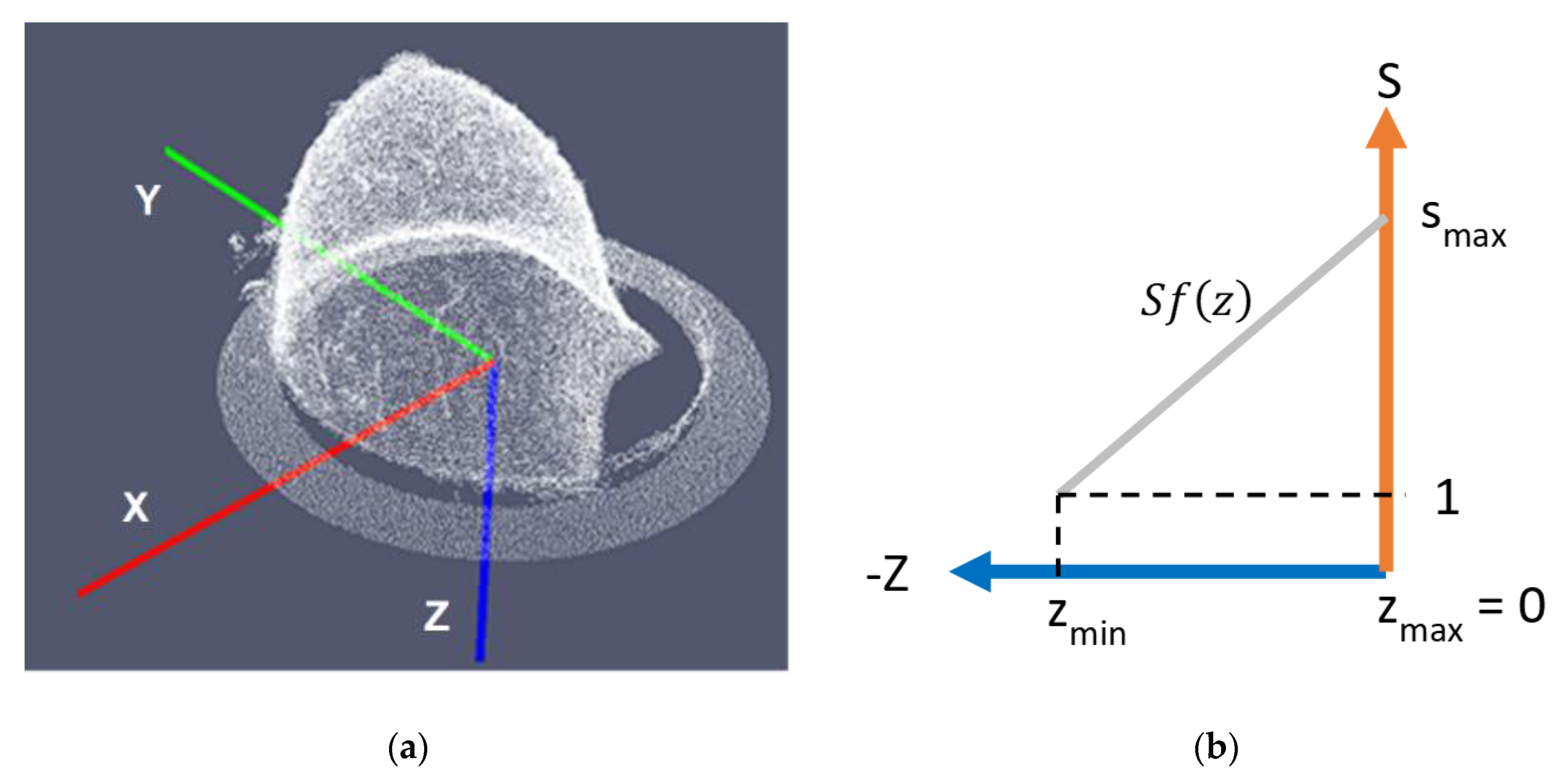
2.3.1. Linear Stretching Procedure

The aim of this processing step is to transform the point cloud $P{c}_B$, obtained after removal of the ring as explained in the previous sub-section, into an elevation point cloud to ensure the generation of a surface with no overlaps (see illustration in the right-hand images in Figure 11a–c). A surface with no overlaps is defined as a surface where there is one single z coordinate for each coordinates pair (x, y).

Overlaps, as defined below, are naturally very common in the geometry of the pendulous breast, especially in the case of elder patients. The stretching of the breast surface, such that it has no overlap, is a processing step which enables the use of 2D image processing methods for de-noising of the point cloud, before meshing. Obviously, the stretching operation is compensated before meshing, such that the original breast shape is ultimately reconstructed.

To perform this transformation, a new origin point $p_{str}$ needs to be defined. This point must be located at the bottom of the breast (close to the chest wall) and the z axis starting from it must intersect the non-stretched surface only once, to successfully stretch the x and y coordinates of the point cloud, as illustrated graphically in Figure 12.

In the following, the procedure put in place to define a linear stretching function $Sf\left(z\right)$ and compute the stretching factor for the x and y coordinates of each point as a function of the z coordinate (see Figure 13b), is detailed. The function is defined in the Wavelia reference coordinate system (see Figure 13a) and it is specified in Equation (11), where $s_{max}$ is the maximal stretching factor, $z_{min}$ and $z_{max}$ are the minimum and maximum z coordinates of the bounding box of $P{c}_B$, and z is the z coordinate of the point to be stretched. $z_{max}$ is equal to zero, as shown in Figure 13b.

$$Sf\left(z\right)=\frac{\left(s_{max}-1\right)}{\left(z_{max}-z_{min}\right)}·z+s_{max}$$

(11)

The following processing steps are applied to compute $s_{max}$:

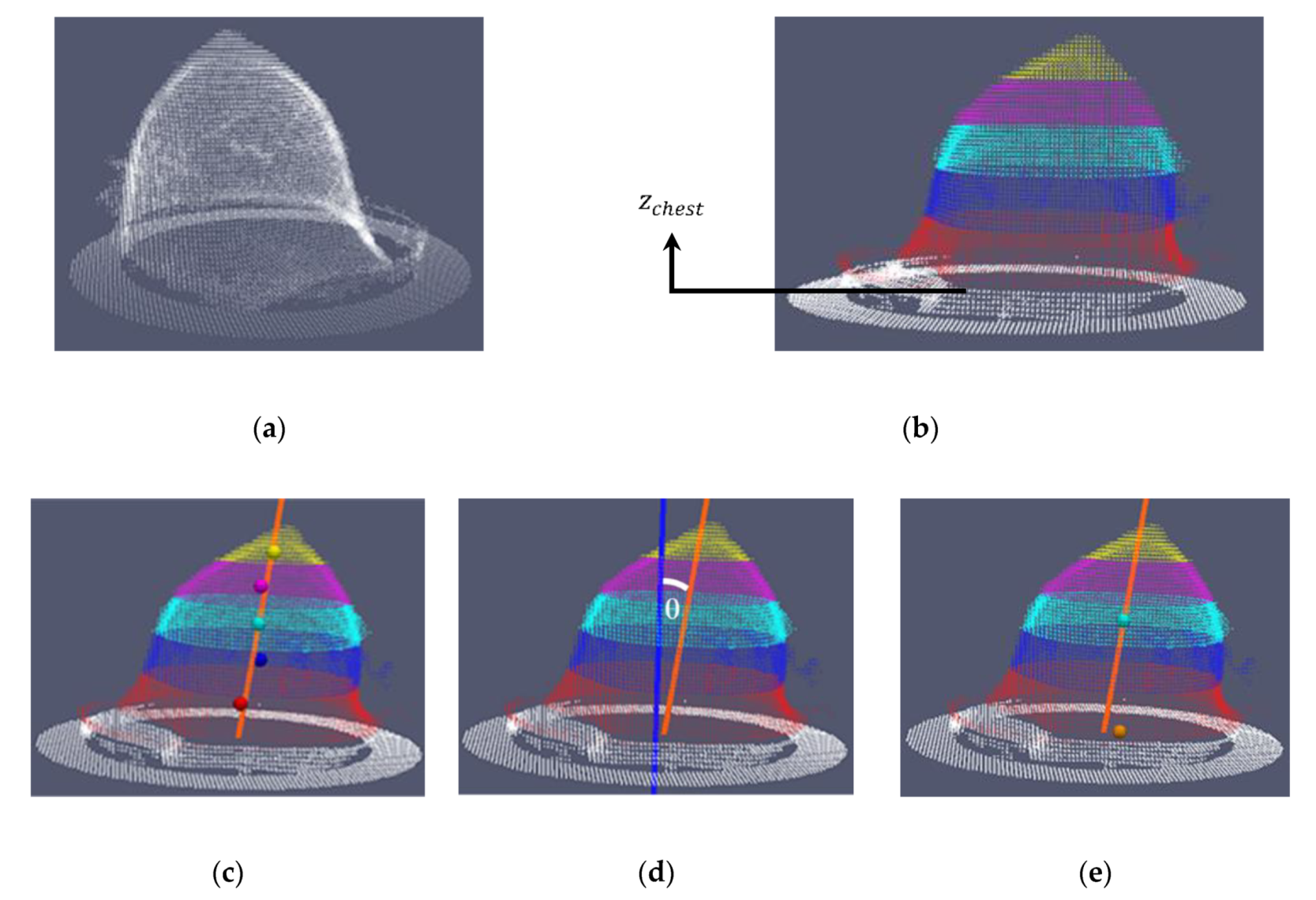
• the number of points of the point cloud is reduced by voxelization (Figure 14a).
• the points associated to the chest wall are removed from the voxelized point cloud, by removing the points where the z-coordinate is in range from 0 to $z_{chest}$ (white points in Figure 14b); $z_{chest}$ has been empirically determined, considering a series of tests on both human and phantom breasts. The aim of this step is to preserve the points corresponding to the pendulous breast.
• the point cloud obtained in the previous step is divided in five vertical sections (red, blue, cyan, magenta and yellow in Figure 14b).
• the orientation axis of the breast is computed, by applying a LS method on the centroids of the five vertical sections (see Figure 14c).
• the θ angle between this axis and the z axis of the Wavelia reference coordinate system is computed (see Figure 14d).
• Finally, $p_{str}$ is determined, by projecting the centroid of the middle section on the orientation axis of the breast (cyan sphere in Figure 14e) and setting to 0 the z coordinate of the projected point. The result corresponds to $p_{str}$ (orange sphere in Figure 14e).

Based on several tests performed both on human and phantom breasts, the minimum stretching value $s_{ref}=8.0$ that can be applied to generate non-overlapping point clouds in all performed tests was determined empirically. The maximum value of the angle θ for which the minimum stretching value $s_{ref} \mathrm{is} \mathrm{applied} \mathrm{by} \mathrm{default}$ has been empirically defined from the same tests. The notation ${\theta }_{ref}$ is used in the sequel of the paper to refer to this value. ${\theta }_{ref}$ is further used to compute the reference value for the tilt of the breast $b\_til{t}_{ref}$ as defined in Equation (12).

$$b\_til{t}_{ref}=1+\tan {\theta }_{ref}$$

(12)

The specific $s_{ref}$ and $b\_til{t}_{ref}$ values can be used to compute the maximal stretching factor $s_{max}$ as defined in Figure 15 and Equation (13), where $b\_tilt$ is the tilt of the breast which is computed by using Equation (12) while ${\theta }_{ref}$ is replaced by θ.

$$s_{max}=\frac{b\_tilt ·s_{ref}}{b\_til{t}_{ref}}$$

(13)

The full procedure to compute $s_{max}$ is presented in Figure 15 above. This procedure ensures that $s_{max}$ is always superior than $s_{ref}$.

Finally, the point cloud $P{c}_B$ is centered at the position $p_{str}$ and the stretching function $Sf\left(z\right)$ is applied (see Equation (11)). The stretched point cloud (right-hand images in Figure 11b,c) is named $P{c}_C$.

2.3.2. Denoising Procedure

Until the previous step, the pendulous breast point cloud has been transformed into an elevation point cloud $P{c}_C$ on the xy plane, while preserving the z coordinates. The aim of the denoising procedure is to remove the artifacts and the ring remaining points and to fill the zones with no points. To do this, the denoising procedure combines morphological information of the pendulous breast, and 2D imaging processing.

At the beginning of this procedure $P{c}_C$ is used to generate a reference rectangular grid for denoising which is then used to perform a first artifacts removal process on $P{c}_C$. To perform this process, the following parameters are used:

• $x_{min}$,$x_{max}$,$y_{min}$ and $y_{max}$: these values correspond to the minimum and maximum x and y coordinates of the bounding box of $P{c}_C$;
• mesh resolution (Dxy): it corresponds to the desired resolution on the xy plane for the 3D breast reconstructed mesh, before the linear stretching transformation (see definition also in Appendix B.2);
• $s_{max}$: this is the maximal stretching factor, as computed in the previous step (see Section 2.3.1);
• $x_{size}$ and $y_{size}$: these are integer values. They correspond to the size of the rectangular grid along the x and y axes after the linear stretching transformation. These values are computed by using Equations (14) and (15), where $Dxy·s_{max}$ corresponds to the stretched mesh resolution, after the stretching transformation. To preserve small parts like the nipple, after the stretching transformation, it was decided to increase the stretched mesh resolution by a factor of 2, as indicated in Equations (14) and (15).

  $$x_{size}=\left[\frac{x_{max}-x_{min}}{Dxy·s_{max}·0.5}\right]$$

  (14)

  $$y_{size}=\left[\frac{y_{max}-y_{min}}{Dxy·s_{max}·0.5}\right]$$

  (15)

By using $x_{size}$ and $y_{size}$ a rectangular grid on the xy plane is generated (see Figure 16b). Each of the z values in the grid (green points in Figure 16a) is computed as the mean value of all the z coordinates of the points located inside the associated small rectangular section (small blue rectangles in Figure 16a). If there are no points inside the small section, the associated z value is set to 0. This ensures a single z coordinate for each coordinates pair (x, y) on the grid.

The obtained rectangular grid can be considered as a 2D image, where the intensity at each point (x,y) corresponds to the z-value (in mm) of the point (x,y,z) in a new stretched point cloud (see Figure 17a). To reduce the noise, remove the larger artifacts and obtain a very smooth grid without completely removing the nipple, a median filter is applied with a large kernel size (11 × 11) to the rectangular grid. The result is the reference rectangular grid for denoising (see Figure 17b). The kernel size (11 × 11) has been selected among various kernel sizes, after testing on a series of both human and phantom breasts (test range from 9 × 9 to 17 × 17).

The signed vertical distance (along the z axis) to the reference rectangular grid for denoising is used as a criterion for the removal of points (positive distance for points above the grid and negative distance for points below the grid). The denoising is performed after splitting the breast into two vertical sections. These are defined in $P{c}_C$ by using the z limit of the nipple section (see Figure 18).

To apply the point removing criterion, the following parameters are defined:

• $z_{min}$ and $z_{max}$: these values correspond to the minimum and maximum z coordinates of the bounding box of $P{c}_C$.
• $z_{nipple}$: this parameter concerns the z limit of the nipple section (see Figure 18). Its value is computed by using Equation (16), where $D{z}_{nipple}$ is an empirically defined value within the range 0 to 1 based on tests performed on human and phantom breasts.

  $$z_{nipple}= z_{min}+ \left(z_{max}-z_{min}\right)·D{z}_{nipple}$$

  (16)
• valid distance: this parameter is applied to the points outside the nipple section. It corresponds to the maximal signed vertical distance to the reference rectangular grid for the denoising operation to preserve points corresponding to the breast surface.
• valid distance for nipple section: this parameter is applied to the points inside the nipple section, where the nipple points are above the breast surface. It corresponds to the maximal signed vertical distance to the reference rectangular grid for the denoising operation to preserve points corresponding to the nipple and areola vicinity on the breast surface.

The removing criterion is applied to $P{c}_C$ by using $z_{nipple}$, valid distance for nipple section and valid distance. The resulting point cloud, after denoising, is named $P{c}_D$. Figure 19a,b illustrates the denoising process applied to the data from two patient scans. In Figure 19, two sample zones (yellow delimited zones) are highlighted before the denoising procedure ($P{c}_C$) and after the denoising procedure ($P{c}_D$). Observing the impact of the denoising procedure on these zones permits to clearly illustrate the efficacy of the denoising procedure to significantly reduce the noise.

When the first artifacts removal process is finalized, $P{c}_D$ is transformed into a full filled rectangular grid $Pc{g}_A$. This point could $Pc{g}_A$ can be considered as a 2D image which allows using 2D imaging processing.

To generate the full filled rectangular grid $Pc{g}_A$ from $P{c}_D$, the size of the rectangular grid is defined in the x and y axes by using Equations (14) and (15). Then, a rectangular grid is generated on the xy plane. To improve the robustness against the noise along the z axis, each of the z values of the grid (green points in Figure 20a) is computed as the median value of all the z coordinates of the points located inside the associated small rectangular section (small blue rectangles in Figure 20a). Some points of the rectangular grid will remain with no defined z value. These points are named “empty points”, and the sections of empty points are named “holes” (see red points in Figure 20b). The points with a defined z value are named “valid points” (see green points in Figure 20b).

To define the z coordinate of the empty points in the rectangular grid (the process to fill the holes), the parameter ring height defined in Appendix B.2 is required. By using this parameter, we divide the valid points of the grid (green points in Figure 21) in two vertical sections: the first one concerns the points the z coordinates of which are in range of 0 to ring height (bright green points in Figure 21), and the second one concerns the points the z coordinates of which are outside the first interval (dark green points in Figure 21). The left-hand image in Figure 21 shows the two sections on the equivalent non-stretched point cloud for a better understanding.

Three types of holes are further defined:

• Type-A hole: the holes bordered by valid points the z coordinates of which are located inside the first interval (bright green points in Figure 22). This type of hole is composed of at least two consecutive empty points along the x axis or along the y axis (see yellow delimited zones in Figure 22). These holes correspond to the zones located between the internal vertical wall of the ring and the border of the breast surface. The z coordinate value of these empty points is set to 0.
• Type-B hole: all the holes not completely bordered by valid points (see Figure 23). These holes correspond to the zones located beyond the ring, where no section of the breast surface is present. The z coordinate value of these empty points is set to 0.
• Type-C hole: the holes bordered by valid points the z coordinates of which are outside the first interval (holes located inside the dark green section).

To fill the type-C holes and the other remaining empty points on the rectangular grid, a bi-linear interpolation is performed by using the closest points for which the z coordinate is defined. Finally, a smoothing procedure is performed by using two b-spline approximations [23]. The first approximation is carried out along the x axis, and the second one is carried out along the y axis. The result is the mean of the two approximations. The resulting point cloud is named $Pc{g}_A$ and it can be considered as a full filled rectangular grid.

At this stage it is possible to use 2D image processing to finalize the denoising procedure. Two 2D processing are performed. The first one is based on erosion and dilation morphological operations by using $Pc{g}_A$ as input. The result is a binary mask, which is applied to $Pc{g}_A$ by a multiplication operation. Then the second one consists in the use of a median filter of several kernel sizes to remove the last remaining artefacts. The final resulting point cloud is named $Pc{g}_C$. (see Appendix C).

2.3.3. Smoothing Step

The aim of this step is to smooth $Pc{g}_C$ while preserving the breast surface details around the nipple. To do this, $Pc{g}_C$ is considered as a 2D image. $Pc{g}_C$ is divided into four vertical sections by using the procedure presented in Appendix C.2, and then a bi-lateral filter [24] is applied with variable kernel size, as defined below:

• a (3 × 3) kernel size for the nipple section (this kernel size allows to smooth this section while sufficiently preserving the breast surface details around the nipple);
• a (5 × 5) kernel size for the second breast section;
• a (7 × 7) kernel size for the third breast section;
• a (9 × 9) kernel size for the fourth breast section.

This, empirically defined, combination of kernel sizes allowed to preserve a good continuity along the four breast sections in all the breast scans we have performed so far. The result is a point cloud we name $Pc{g}_D$.

2.3.4. Meshing Procedure

$Pc{g}_D$ is a rectangular grid that can be easily presented as a 2D matrix of 3D points. A triangular mesh is further generated, where the points of each triangle are connected in clockwise order, as illustrated in Figure 24.

To perform the final meshing, we compute the inverse of the stretching function earlier presented in Section 2.3.1, as defined in Equation (17). Then, we apply Equation (17) to the points of the grid, and finally the point $p_{str}$ is added, such that the original position of the breast is retrieved.

$$Sf{\left(z\right)}^{-1}=\frac{1}{Sf\left(z\right)}=\frac{1}{\frac{\left(s_{max}-1\right)}{\left(z_{max}-z_{min}\right)}·z+s_{max}}$$

(17)

Indicative results of the meshing procedure are presented in Figure 25.

2.3.5. Breast Volume Computation

To compute the volume of the 3D triangular mesh of the patient’s breast (Final Mesh) generated in the previous step we use as reference the cumulative method presented by Zhang and Chen [25] but instead of using a tetrahedron as elementary calculation object, we use a truncated triangular prism [26], which is perpendicular to the xy plane (see Figure 26). This condition permits to reduce the number of arithmetic operations.

The signed volume V of the elementary truncated triangular prism is computed for each triangle ($p_a$, $p_b$, $p_c$ in Figure 26) by using Equation (18), where A is the area of the basis of the truncated triangular prism and sign corresponds to the sign (1 or −1) of V. The value of sign is determined by the inner product $\overrightarrow{n_{abc}}.{\widehat{e}}_z$, where ${\widehat{e}}_z$ is the unitary vector (0,0,1) defining the orientation of the z axis in the Wavelia reference coordinate system (see Figure 26).

$$V=\left(A ·\frac{\left(\left| z_1\right|+\left| z_2\right|+\left| z_3\right|\right)}{3}\right)·sign$$

(18)

where:

$$A=\left|\frac{x_1·\left(y_2-y_3\right)+x_2·\left(y_3-y_1\right)+x_3·\left(y_1-y_2\right)}{2}\right|$$

To compute the total volume of Final Mesh we use Equation (19).

$$V_{total}=\left|{{\displaystyle \sum }}^{}{V}_i\right|$$

(19)

where: $V_i=\left(A_i ·\frac{\left(\left| z_{i1}\right|+\left| z_{i2}\right|+\left| z_{i3}\right|\right)}{3}\right)·sig{n}_i$, $A_i=\left|\frac{x_{i1}·\left(y_{i2}-y_{i3}\right)+x_{i2}·\left(y_{i3}-y_{i1}\right)+x_{i3}·\left(y_{i1}-y_{i2}\right)}{2}\right|$ and i stands for the index of triangles of elementary truncated triangular prisms. $\left(x_{i1}, y_{i1}, z_{i1}\right)$, $\left(x_{i2}, y_{i2}, z_{i2}\right)$ and $\left(x_{i3}, y_{i3}, z_{i3}\right)$ are the 3D coordinates of the vertices associated with the triangle i.

2.4. Description of the Method to Quantify the 3D Breast Surface Reconstruction Accuracy

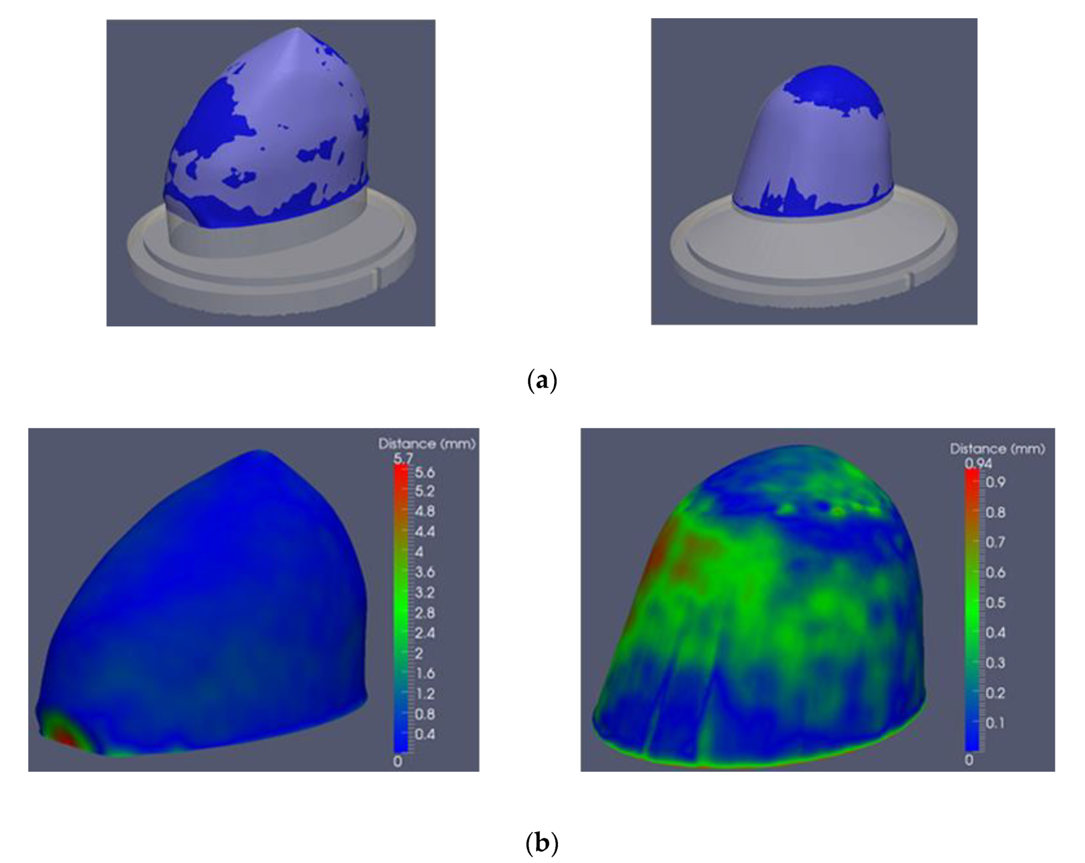
2.4.1. Generation of 3D Breast Reference Surfaces

To assess the accuracy of the 3D breast surface reconstruction and the breast volume computation, two MRI-based 3D printed breast phantoms named B1 and B2 have been used. The two anthropomorphic breast phantoms, which have been also used all along the Wavelia prototype medical device design, experimental testing and validation, are presented in Figure 27. As detailed in [6], the geometry of the phantoms which have been manufactured in-house by MVG Industries for this purpose, originated from real MRI images of patients, publicly made available by the University of Wisconsin (UWCEM database) [27].

Before starting the comparison procedure, a pre-processing step was performed on the 3D breast phantom representations in order to extract the external surface of each breast phantom (see Figure 28). To perform the pre-processing step, the MeshLab open source software has been used [28]. The resulting reference breast phantom representations have been named Model_B1_Ref and Model_B2_Ref.

Model_B1_Ref and Model_B2_Ref have been further on used to assess the accuracy of the 3D breast surface reconstruction, the estimation of the vertical extent of the breast and the estimation of the volume of the breast, as performed by the Wavelia OBCD subsystem. Figure 29 shows two indicative results of the Wavelia 3D reconstruction method (see Section 2.3).

2.4.2. Procedure to Quantify the Accuracy of the 3D Breast Surface Reconstruction

To quantify the accuracy of the 3D breast surface reconstruction method and the breast volume computation, we first extract the part of the reconstructed surface that corresponds to the breast surface (removal of the flat horizontal surface corresponding to the examination table). To perform this operation, the Wavelia reference coordinate system is used, as presented in Section 2.1, to define the z value of the cutting plane that will be used to extract the breast surfaces (see Figure 30).

The extraction procedure of the breast surfaces has been performed using the Paraview software [29]. After the breast surface has been extracted, a rigid registration is applied between this surface and its breast reference model. The Wavelia reference coordinate system is used as the main reference system for this operation. This procedure is performed by using the ICP (Iterative Closest Point) method, which is integrated in the MeshLab software [28]. The ICP transformation is applied to the breast reference model in order to obtain the registered breast reference model. The result of the registration procedure is shown in Figure 31a, where the extracted breast surface appears in blue and the registered breast reference model appears in semi-transparent grey. Then, the MeshLab software is used to compute the unsigned distance from each point of the extracted breast surface to the closest point of the registered breast reference model (distance error). We used the distance error as point color criterion to generate the breast distance color map of the extracted breast surface by using the MeshLab software as well (Figure 31b). Based on the distance data of the extracted breast surfaces, we also computed the following parameters to assess the accuracy of either 3D breast surface reconstruction:

• percentage of points with distance error less or equal to 0.5 mm;
• percentage of points with distance error less or equal to 1.0 mm;
• percentage of points with distance error less or equal to 1.5 mm;
• Root Mean Square (RMS) distance error in mm.

After the rigid registration has been performed, the breast reference surface is extracted from the registered breast reference model by using a cutting plane coinciding with the lower surface of the examination table. The breast reference surface is a closed surface.

Then, the vertical extent and the volume of the breast reference surface are computed by using the MeshLab software [28]. These parameters have been named: reference breast height ($H_{ref}$) and reference breast volume ($V_{ref}$). The following metrics are used to assess the accuracy of the vertical extent ($H_{comp}$) and the volume ($V_{comp}$) of the breast, as computed by the Wavelia OBCD subsystem:

• Breast vertical extent error [mm]: this metric is defined as: $H_{comp}-H_{ref}$.
• Breast volume error [mL]: this metric is defined as: $V_{comp}-V_{ref}$.
• Breast volume error in percentage: this metric is defined as: $\left(\frac{V_{comp}-V_{ref}}{V_{ref}}\right)·100$.

3. Results and Discussion

3.1. Calibration Evaluation

Several tests of the calibration procedure have been performed with the Wavelia OBCD subsystem. Indicative values of the calibration transform error, as evaluated during these tests, are presented in

Table 1. Performance results of calibration procedure tests.

Test ID	Calibration Transform Error (mm)
1	1.40
2	0.58
3	0.70
4	0.97
5	0.88
6	0.80

.

Table 1 reports a value greater than 1 mm for the calibration transform error, in the case of Test 1. Such a relatively high value of the calibration transform error could be due to small movements of the cross-shaped reference object during the azimuthal 3D scan of the camera. To prevent these movements and to ensure sub-millimetric precision in the computation of the calibration transform, it is very important to avoid any contact with the OBCD subsystem during the calibration azimuthal scan of the camera.

Test 1 was one of the first tests of the calibration method with the Wavelia prototype, while it was still at the factory. All the other reported tests (Test 2 to Test 6) have been performed after installation of the Wavelia system at the Galway University Hospital, while carrying-out the calibration procedure after repeated training. It is demonstrated that sub-millimetric precision of the method has been consistently assured, after validation of the system for transfer to the clinical investigation site.

It is worthwhile noting that, this being a prototype version 1 of the Wavelia system, installed in the hospital for a first-in-human clinical investigation, the calibration is meant to be performed by trained technical staff during installation or maintenance of the system. It is not meant to be repeated by the daily operator, during the clinical investigation. The calibration measurements are used to define once the cumulative transformation operator, which is afterwards applied to align the multi-view camera measurements of all breast scans. The required accuracy for the calibration measurement (controlled environment) is higher than the effective accuracy of the breast scan measurements, such that the cumulative transformation operator is optimally defined.

3.2. D Breast Surface Reconstruction: Quantitative Evaluation Results

A series of eight 3D breast reconstruction tests have been performed. Six of the tests were performed on breast phantoms fully introduced into the opening of the examination table (four tests for B1 phantom and two tests for B2 phantom). To simulate a smaller breast phantom, the two remaining 3D breast reconstructions were performed with the B2 breast phantom partially introduced into the opening of the examination table. The results of the eight tests are shown in Figure 32 and

Table 2. Summary of the accuracy results on eight 3D breast surface reconstruction tests involving the B1 and B2 breast phantoms.

	B1 Test 1	B1 Test 2	B1 Test 3	B1 Test 4	B2 Test 1	B2 Test 2	B2 Test 3	B2 Test 4
Total number of points on the extracted breast surface	177,228	178,570	178,562	179,896	134,808	137,000	119,758	119,748
Percentage of points with distance error <= 0.5 mm (%)	76.80	90.20	89.01	87.28	82.18	93.77	83.88	79.88
Percentage of points with distance error <= 1.0 mm (%)	96.26	95.19	94.58	97.45	100	99.14	98.12	99.77
Percentage of points with distance error <= 1.5 mm (%)	97.55	97.42	97.37	98.94	100	100	99.86	99.93
Percentage of points with distance error >1.5 mm (%)	2.45	2.58	2.63	1.06	0.00	0.00	0.14	0.07
RMS distance error (mm)	0.74	0.65	0.69	0.50	0.40	0.30	0.44	0.42
Reference Vertical Extent of the Breast (mm)	110.19	110.96	110.96	111.16	84.67	84.97	67.88	67.59
Computed Vertical Extent of the Breast (mm)	109.36	109.55	109.60	109.85	84.71	84.79	67.73	67.50
Error in the Vertical Extent of the Breast (mm)	−0.83	−1.41	−1.36	−1.31	0.04	−0.19	−0.15	−0.09
Reference Volume of the Breast (mL)	915.57	924.57	924.57	928.28	498.92	502.51	349.48	350.01
Computed Volume of the Breast (mL)	909.81	921.25	921.25	921.97	494.27	502.21	349.51	347.48
Breast Volume Error (mL)	−5.75	−3.31	−3.31	−6.31	−4.64	−0.31	0.03	−2.52
Breast Volume Error (%)	−0.63	−0.36	−0.36	−0.68	−0.93	−0.06	0.01	−0.72

.

The breast distance maps shown in Figure 32 demonstrate the homogeneous spatial distribution of the points with a distance inferior or equal to 1.0 mm. Figure 32 also confirms the limited extension of the zones where the distance error is greater than 1.5 mm.

Table 2 shows that at least 76% of the extracted breast surface has a distance error inferior or equal to 0.5 mm, that at least 94% of this surface has a distance error inferior or equal to 1.0 mm and at least 97% of this surface has a distance error inferior or very close to 1.0 mm (greater than 1.0 mm and less or equal to 1.5 mm). It also shows that only approximately 3% of the extracted breast surface has a distance error greater than 1.5 mm. Based on these results, we can affirm that globally the accuracy of the extracted breast surface is sub-millimetric. This sub-millimetric accuracy may be also deduced from the RMS distance error which is overall less than 0.75 mm.

Concerning the computation of the vertical extent of the pendulous breast, Table 2 shows that the computed breast vertical extent is generally underestimated (breast vertical extent error is often negative) and that the absolute breast vertical extent error is very close to 1.0 mm (worst-case error of −1.41 mm for B1 test 2 in Table 2).

Table 2 also shows that the computed breast volume tends also to be underestimated (volume error is often negative) and that the uncertainty in the breast volume computation is less than 1%.

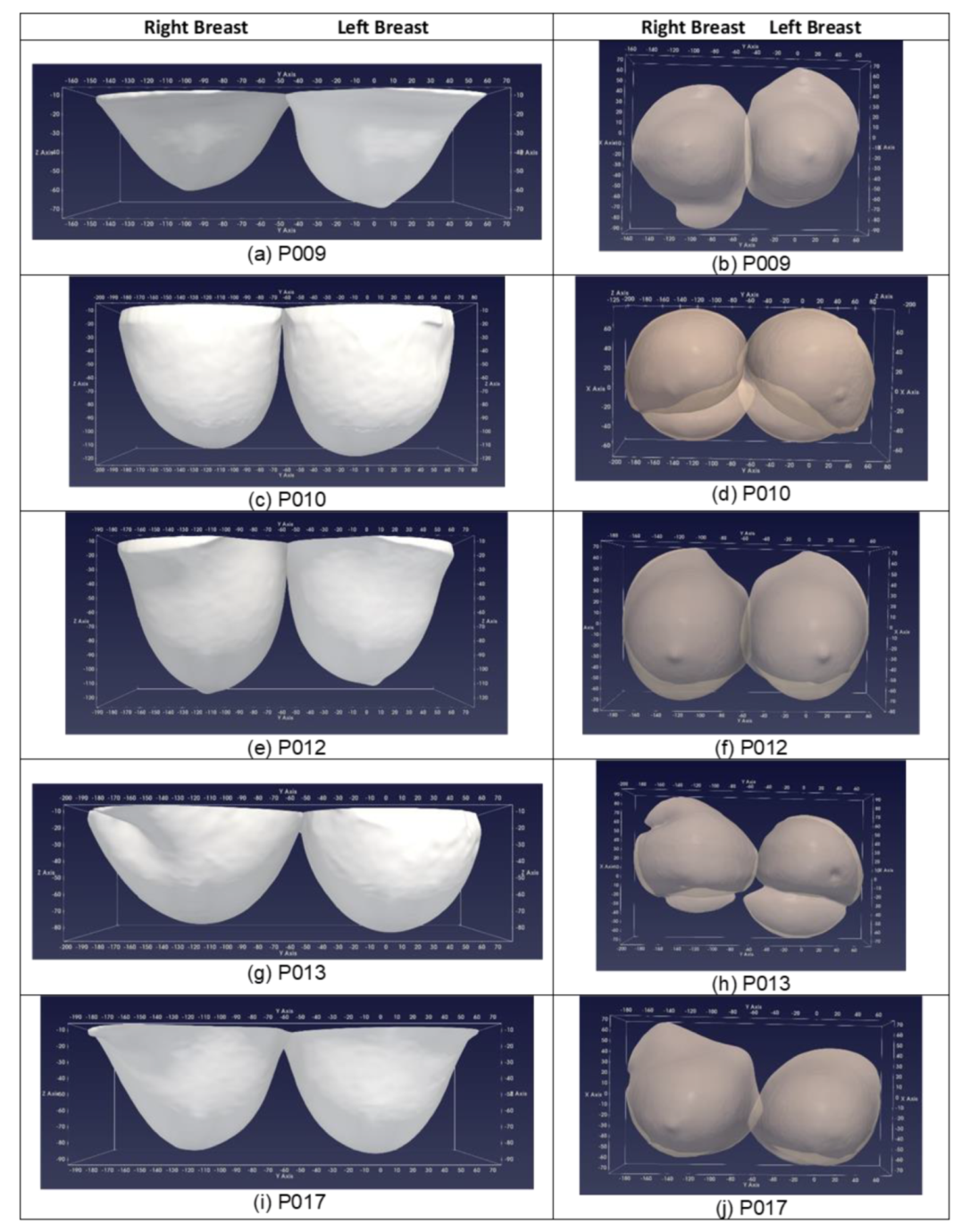
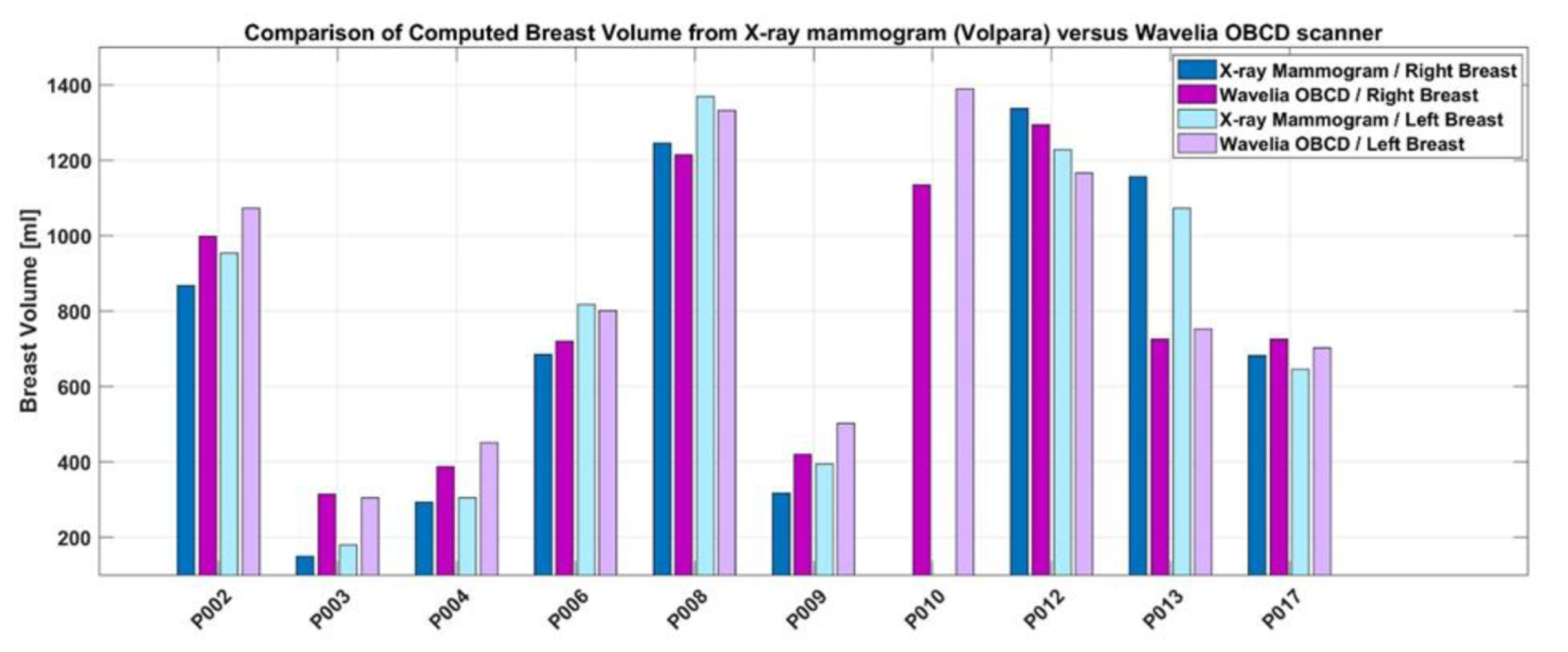
3.3. D Breast Surface Reconstruction: Indicative Results from the First Ten Patient Scans

In Figure 33 and Figure 34, the reconstructed breast surfaces using the Wavelia OBCD subsystem are shown for the ten first patients enrolled in the on-going first in-human clinical investigation of the Wavelia system, at Galway University Hospital. These are preliminary clinical results which serve to demonstrate the efficacy of the presented calibration algorithm and 3D breast surface reconstruction method on real clinical data. It is demonstrated that meaningful breast surfaces of good quality have been achieved for all the ten patient scans.

In Figure 33 and Figure 34, two views of the reconstructed surface of both breasts of each patient are shown. The two selected views for this illustration are: (a) a side view of the two pendulous breasts: looking at the patient from the front; (b) a supine-mimicking view of the two breasts: looking at the patient from the bottom. This comparative presentation of the breast anatomy for this group of ten patients, as captured during their Wavelia OBCD scans, highlights the expected variability in the positioning of the patients. Even though the same positioning of the arms and alignment of the patient’s body with the bed is intended in all cases, unavoidable rotations of the breasts and/or twist of the torso seem to happen in the case of some patients.

While a quantitative evaluation of the reconstructed surfaces is not straightforward in the case of the patient scans, the computation of the breast volume, as performed using the Wavelia OBCD scan data, has been possible to be validated using as reference the X-ray mammography breast volume data, being made available for the same patients.

All the patients enrolled in the clinical study have had an X-ray mammogram performed no more than 6 weeks ahead of their scan with the Wavelia prototype medical device. The mammograms have been processed with the Volpara VDM (Volumetric Density Measurement) software package [30] and the breast volume has been computed. The Volpara VDM breast volume and density computation have been extensively validated, against MRI breast volume and density estimation [31,32,33,34] and can be safely considered as a valid reference. In [33] breast volume estimates obtained from 186 FFDM (Full Filed Digital Mammography) exams including mediolateral oblique (MLO) and cranial-caudal (CC) views to objective reference standard measurements obtained from breast MRI have been presented. The Pearson’s correlation coefficient between the two computations of the breast volume has been found to be as high as 0.97. The Volpara commercial software was used to compute the breast volume and volumetric breast density, based on FFDM data, in this study. In [34], the agreement of three mammographic techniques (Single-energy X-ray Absorptiometry [SXA], Quantra, and Volpara) with MRI for percent fibro-glandular tissue volume, absolute fibro-glandular tissue volume, and total breast volume computation was assessed. In terms of breast volume computation, the squared Pearson’s correlation coefficient was reported to be 0.91 between all the three mammographic techniques and the MRI, while the achieved RMSE (Root Mean Squared Error) was found to be 108 mL, 109 mL and 121 mL for the three mammographic methods correspondingly, when compared to MRI. This study involved data from 99 women. Both referenced studies have been used to validate volumetric breast density and also breast volume computation using FFDM data, the validation being performed against computation using 3D MRI data.

A similar approach has been adopted in our study to validate breast volume computation using the Wavelia OBCD 3D data, against the computation performed by the already validated Volpara software on the available FFDM data. Results on the 10 first patients that have participated in the first-in-human clinical investigation of the Wavelia system are presented. In Figure 35, the volume of both breasts of each of the ten patients is plotted, as computed from either:

• the Wavelia OBCD 3D scan data, or
• the 2D X-ray mammogram (Volpara software package, computation on ‘For processing’ DICOM files of the two standard mammographic views – Cranio-Caudal and Medio-Lateral Oblique).

Good level of correspondence between the breast volume computation, as performed by the two distinct imaging modalities, is demonstrated, thus validating the Wavelia OBCD breast surface reconstruction and volume computation. It is interesting to observe that the RMSE error computed between the Wavelia OBCD and FFDM (Volpara) breast volume computations based on this first small dataset of patients is 154.6 mL, thus in the same order of magnitude as the RMSE reported in [34] between FFDM and MRI.

Significant discrepancy between the X-ray mammography and the Wavelia OBCD breast volume computation can be noticed only in the case of Patient 013 (P013). This has most probably been due to the patient not being well positioned on the Wavelia scanner, resulting in part of her breasts not being scanned. Patient 003 had very small breasts, potentially difficult to be fully inserted in-between the X-ray mammography plates, resulting in under-estimation of the breast volume by the X-ray mammography in this case. The ‘for processing’ DICOM files, which are required for processing the mammograms with Volpara VDM, were not available in the case of Patient 010.

Finally, in order to evaluate the impact of potential movement of the patient’s breast during the OBCD scan, a quality check has been developed and executed after each OBCD patient scan. For the purpose of the quality check, two versions of the breast surface are reconstructed using two interlaced and non-overlapping subsets of the full set of recorded azimuthal samples (Subset 1: camera at the azimuthal positions {0:60:300}°, Subset 2: camera at the azimuthal positions {30:60:330}°). The OBCD scan is validated, as long as the RMS distance between the two surfaces is inferior to 0.8 mm. The OBCD scans of all the patients participating in the first clinical investigation so far have been validated with this criterion, which indicates that if sub-millimetric precision has been demonstrated in the case of static breast phantoms, the same level of precision can be maintained during the OBCD scan of a real breast. Obviously, before the scan starts, the patient is instructed by the research assistant to stay still, avoid heavy breathing and maintain a relaxed position during the total duration of the scan, which lasts approximately 1 min.

3.4. Wavelia OBCD Breast Surface Reconstruction: Towards Development of a Real-Time Support Tool for the Wavelia MBI Examination and Breast Cancer Diagnosis

As specified in the introduction, in the first prototype of the Wavelia breast imaging medical device, the OBCD and MBI subsystems are integrated in two separate examination tables on which the two scans are sequentially performed, while the patient positions herself in approximately the same way during both examinations. The OBCD scan is performed while the breast is hanging in the air, while the MBI scan is performed with the breast being immersed in a coupling (or transition) creamy liquid, which is opaque.

Given this implementation, at this stage of development of the Wavelia system, the breast surface reconstruction using the OBCD subsystem serves to define the amount of transition liquid to be used for the MBI scan and also to define the length of the vertical scan of the pendulous breast with the MBI system. In the context of the first-in-human clinical study of the Wavelia breast imaging medical device, it has also served to verify the correspondence of the breast anatomy, as retrieved using two distinct imaging modalities (Wavelia OBCD and MBI), tested for the first time on humans.

Rigid registration is performed to match the reconstructed breast surfaces, as computed during the two scans (OBCD and MBI). The ultimate objective of this operation is to exploit the sub-millimetric level of detail of the OBCD-derived breast surface, as a high-quality envelope for the MBI-derived breast abnormality detections for breast cancer diagnosis. It is recalled that due to the physically limited spatial resolution that can be achievable at the microwave frequency range, the exact orientation of the pendulous breast under scan, as well as details such as the nipple location, cannot be defined using the MBI-derived reconstruction of the breast surface alone. With no access to such level of detail, the annotation of the breast quadrant and clock-position at which an abnormality has been detected with MBI cannot be very accurate either, when using the MBI system stand-alone.

Given the potential deformation of the breast when submerged in the transition liquid, the exploitation of the OBCD breast surface for refined localization of the detected breast abnormalities with MBI is possible only in the case of minimally deformed breasts, in the actual implementation. In Figure 36a, the example of a young patient (37 years old) with medium-sized breasts, which have not been significantly deformed when immersed in the transition liquid, is shown. For such a patient, the registered OBCD contour can be safely used as envelope for the breast abnormalities, as detected with MBI. In Figure 36b, the example of an elderly patient (68 years old) with large breasts, which have been significantly deformed when immersed in the transition liquid, is shown. This second patient is a case in which the simple rigid registration of the OBCD-derived breast surface is not usable as an envelope for the breast abnormalities, as detected with MBI, in the actual implementation of the system.

In a future generation of the Wavelia breast imaging medical device prototype, it is planned to integrate both the OBCD and MBI subsystems in the same examination table, such that both scans are performed while the patient stays at the exact same position and the breast is in the exact same ambient conditions. A semi-transparent transition liquid would then need to replace the actual creamy and opaque transition liquid, such that the OBCD scan can be performed in the same conditions as the MBI scan and the breast is identically deformed during both scans. With such a future version of the Wavelia system, the OBCD-derived breast surface reconstruction is meant to enhance significantly the potential of the Wavelia Microwave Breast Imaging system in terms accurate localization of the detected breast abnormalities in the patient’s breast, no matter what the level of breast deformation due to immersion in the transition liquid is. In addition, while being practically real-time available, the OBCD breast surface reconstruction is meant to drive the operator during the positioning of the patient (e.g., improve the centering of the breast in the system), such that the MBI scan can be performed in the best possible conditions.

4. Conclusions

In this paper, a new calibration algorithm for turntable-based 3D scanning systems, a new method for 3D surface reconstruction from point cloud based on a linear stretching function, and a breast volume computation method, which have been designed for and integrated in the OBCD subsystem of the Wavelia prototype breast imaging medical device, have been thoroughly presented. Indicative experimental results with two test breast phantoms and preliminary results from ten patient scans have demonstrated the efficacy of the system in reconstructing with high precision the external envelope of a female patient’s breast hanging below the examination table, while the patient is in prone position. This consists in very valuable input information for the second counterpart of the Wavelia medical device, the MBI subsystem, which aims at detecting the presence of breast pathologies, based on the contrast, in terms of dielectric properties, between healthy and malignant breast tissue.

The envelope of the breast being scanned with the microwave breast imaging system is essential to be known for any detection in the microwave image to be meaningfully referenced in space. In addition, specifically for microwave breast imaging, as the dielectric properties of the interior of the breast are unknown, while the dielectric properties of the transition medium are known, the breast envelope which is extracted at first also serves as boundary between the two electromagnetic wave propagating media (dielectrically known exterior of the breast versus dielectrically unspecified interior of the breast), which is very important a priori information for any microwave imaging algorithm, further on. The spatial resolution of the OBCD (optical) subsystem is significantly finer than the one of the MBI (microwave) subsystem, but the optical subsystem cannot penetrate the breast skin, while the microwave subsystem can. The interest in fusing the optical and microwave data is exactly to profit from a highly detailed breast envelope, as spatial reference for any abnormalities of the breast tissues being detectable with microwaves.

The Wavelia prototype medical device has only recently been installed at the Galway University Hospital, Ireland, for its first-in-human pilot clinical test. To this day, the system has been tested on twenty patients in total (the aim being to test it on thirty patients by the end of this first-in-human clinical investigation). The OBCD subsystem, which has been the main focus of this paper, has been evaluated positively by the users, so far, and generated reliable data which are being efficiently exploited in the ongoing off-line processing of the MBI subsystem datasets. A first encouraging patient result, involving the detection of a palpable Invasive Ductal Carcinoma (IDC) of approximate size 15 mm in the breast of a 44-year old patient, using the Wavelia breast imaging medical device, has been presented in [35]. More complete associated clinical data results will be included in future publications on the Wavelia Microwave Breast Imaging system.

The proposed method for new 3D surface reconstruction from point clouds has been designed based on the shape of the breast when the patient is in prone position on the examination table (Wavelia MBI and OBCD subsystems). However, beyond this specific application, the method could be also used to reconstruct objects other than the breast, as long as the object is representable with the shape of a cone or a cylinder (e.g., the breast can be represented by a cone). The proposed calibration method could be used to calibrate any turntable-based 3D scanning system, in general.

References

1. Fear, E.C.; Meaney, P.M.; Stuchly, M.A. Microwaves for Breast Cancer Detection? IEEE Potentials 2003. [Google Scholar] [CrossRef]
2. O’Loughlin, D.; O’Halloran, M.; Moloney, B.M.; Glavin, M.; Jones, E.; Elahi, M.A. Microwave breast imaging: Clinical advances and remaining challenges. IEEE Trans. Biomed. Eng. 2018, 65, 2580–2590. [Google Scholar] [CrossRef] [PubMed]
3. Fasoula, A.; Duchesne, L.; Cano, J.G.; Lawrence, P.; Robin, G.; Bernard, J.-G. On-Site Validation of a Microwave Breast Imaging System, before First Patient Study. Diagnostics 2018, 8, 53. [Google Scholar] [CrossRef] [PubMed] [Green Version]
4. Iversen, P.O.; Garreau, P.; Burrell, D. Real-time spherical near-field handset antenna measurements. IEEE Antennas Propag. Mag. 2001. [Google Scholar] [CrossRef]
5. Fasoula, A.; Anwar, S.; Toutain, Y.; Duchesne, L. Microwave vision: From RF safety to medical imaging. In Proceedings of the 2017 11th European Conference on Antennas and Propagation, EUCAP, Paris, France, 19–24 March 2017. [Google Scholar] [CrossRef]
6. Fasoula, A.; Bernard, J.; Robin, G.; Duchesne, L. Elaborated breast phantoms and experimental benchmarking of a microwave breast imaging system before first clinical studyTitle. In Proceedings of the 12th European Conference on Antennas and Propagation, London, UK, 9–13 April 2018. [Google Scholar]
7. Registered Cinical Trial Protocol. Available online: https://clinicaltrials.gov/ct2/show/NCT03475992 (accessed on 11 February 2020).
8. Lawrence, P.; Fasoula, A.; Duchesne, L. RF-based Breast Surface Estimation—Registration with Reference Imaging Modality. In Proceedings of the 2018 IEEE International Symposium on Antennas and Propagation & USNC/URSI National Radio Science Meeting, Boston, MA, USA, 8–13 July 2018. [Google Scholar]
9. Winters, D.W.; Shea, J.D.; Madsen, E.L.; Frank, G.R.; van Veen, B.D.; Hagness, S.C. Estimating the breast surface using UWB microwave monostatic backscatter measurements. IEEE Trans. Biomed. Eng. 2007. [Google Scholar] [CrossRef]
10. Sakamotov, T.; Sato, T. A target shape estimation algorithm for pulse radar systems based on boundary scattering transform. IEICE Trans. Commun. 2004. [Google Scholar] [CrossRef]
11. Endo, F.; Kidera, S. Accuracy enhanced beamforming method based on envelope surface extraction for non-contact UWB breast cancer radar. In Proceedings of the ISAP 2016—International Symposium on Antennas and Propagation, Okinawa, Japan, 24–28 October 2016. [Google Scholar]
12. Sarafianou, M.; Preece, A.W.; Craddock, I.J.; Klemm, M.; Leendertz, J.A. Evaluation of Two Approaches for Breast Surface Measurement Applied to a Radar-Based Imaging System. IEEE Trans. Antennas Propag. 2016. [Google Scholar] [CrossRef] [Green Version]
13. Williams, T.C.; Bourqui, J.; Cameron, T.R.; Okoniewski, M.; Fear, E.C. Laser surface estimation for microwave breast imaging systems. IEEE Trans. Biomed. Eng. 2011. [Google Scholar] [CrossRef]
14. Kurrant, D.; Bourqui, J.; Fear, E. Surface estimation for microwave imaging. Sensors 2017, 7, 1658. [Google Scholar] [CrossRef] [Green Version]
15. Lee, W.Y.; Kim, M.J.; Lew, D.H.; Song, S.Y.; Lee, D.W. Three-dimensional surface imaging is an effective tool for measuring breast volume: A validation study. Arch. Plast. Surg. 2016. [Google Scholar] [CrossRef] [Green Version]
16. Chae, M.P.; Rozen, W.M.; Spychal, R.T.; Hunter-Smith, D.J. Breast volumetric analysis for aesthetic planning in breast reconstruction: A literature review of techniques. Gland. Surg. 2016. [Google Scholar] [CrossRef]
17. Choppin, S.B.; Wheat, J.S.; Gee, M.; Goyal, A. The accuracy of breast volume measurement methods: A systematic review. Breast 2016. [Google Scholar] [CrossRef]
18. O’Connell, R.L.; Khabra, K.; Bamber, J.C.; deSouza, N.; Meybodi, F.; Barry, P.A.; Rusby, J.E. Validation of the Vectra XT three-dimensional imaging system for measuring breast volume and symmetry following oncological reconstruction. Breast Cancer Res. Treat. 2018. [Google Scholar] [CrossRef] [PubMed] [Green Version]
19. Khawaldeh, S.; Aleef, T.A.; Pervaiz, U.; Minh, V.H.; Hagos, Y.B. Complete End-to-End Low Cost Solution to a 3D Scanning System with Integrated Turntable. Int. J. Comput. Sci. Inf. Technol. 2017. [Google Scholar] [CrossRef]
20. Song, T.; Zhou, L.; Ding, X.; Yi, W. 3D Surface Reconstruction Based on Kinect Sensor. Int. J. Comput. Theory Eng. 2013. [Google Scholar] [CrossRef] [Green Version]
21. Ye, Y.; Song, Z. An accurate 3D point cloud registration approach for the turntable-based 3D scanning system. In Proceedings of the 2015 IEEE International Conference on Information and Automation, ICIA, Lijiang, China, 8–10 August 2015. [Google Scholar] [CrossRef]
22. Xiao, W.; Deng, M.; Li, C. A surface reconstruction algorithm based on 3D point cloud stratified sliced. Sens. Transducers 2014, 173, 197. [Google Scholar]
23. Rankin, J.R. Computer Graphics Software Construction; Prentice Hall of Australia: Sydney, Australia, 1989; ISBN 0-7248-0194-9. [Google Scholar]
24. Tomasi, C.; Manduchi, R. Bilateral filtering for gray and color images. In Proceedings of the IEEE International Conference on Computer Vision, Bombay, India, 7 January 1998. [Google Scholar] [CrossRef]
25. Zhang, C.; Chen, T. Efficient feature extraction for 2D/3D objects in mesh representation. In Proceedings of the IEEE International Conference on Image Processing, Thessaloniki, Greece, 7–10 October 2001. [Google Scholar] [CrossRef]
26. Klamkin, M.S. On the Volume of a Class of Truncated Prisms and Some Related Centroid Problems. Math. Mag. 1968. [Google Scholar] [CrossRef]
27. Zastrow, E.; Davis, S.K.; Lazebnik, M.; Kelcz, F.; van Veen, B.D.; Hagness, S.C. Development of anatomically realistic numerical breast phantoms with accurate dielectric properties for modeling microwave interactions with the human breast. IEEE Trans. Biomed. Eng. 2008. [Google Scholar] [CrossRef] [Green Version]
28. Cignoni, P.; Callieri, M.; Corsini, M.; Dellepiane, M.; Ganovelli, F.; Ranzuglia, G. MeshLab: An open-source mesh processing tool. In Proceedings of the 6th Eurographics Italian Chapter Conference, Salerno, Italy, 2–4 July 2008. [Google Scholar]
29. Ahrens, J.; Geveci, B.; Law, C. ParaView: An end-user tool for large-data visualization. In Visualization Handbook; Elsevier: Amsterdam, The Netherlands, 2005; ISBN 978-0123875822. [Google Scholar]
30. Highnam, R.; Brady, M.; Yaffe, M.J.; Karssemeijer, N.; Harvey, J. Robust breast composition measurement—VolparaTM. In International Workshop on Digital Mammography; Springer: Berlin, Germany, 2010. [Google Scholar] [CrossRef]
31. Brandt, K.R.; Scott, C.G.; Ma, L.; Mahmoudzadeh, A.P.; Jensen, M.R.; Whaley, D.H.; Wu, F.F.; Malkov, S.; Hruska, C.B.; Norman, A.D.; et al. Comparison of Clinical and Automated Breast Density Measurements: Implications for Risk Prediction and Supplemental Screening. Radiology 2016. [Google Scholar] [CrossRef] [Green Version]
32. Ko, S.Y.; Kim, E.-K.; Kim, M.J.; Moon, H.J. Mammographic density estimation with automated volumetric breast density measurement. Korean J. Radiol. 2014. [Google Scholar] [CrossRef] [Green Version]
33. Gubern-Mérida, A.; Kallenberg, M.; Platel, B.; Mann, R.M.; Martí, R.; Karssemeijer, N. Volumetric breast density estimation from full-field digital mammograms: A validation study. PLoS ONE 2014. [Google Scholar] [CrossRef] [PubMed]
34. Wang, J.; Azziz, A.; Fan, B.; Malkov, S.; Klifa, C.; Newitt, D.; Yitta, S.; Hylton, N.; Kerlikowske, K.; Shepherd, J.A. Agreement of mammographic measures of volumetric breast density to MRI. PLoS ONE 2013. [Google Scholar] [CrossRef] [PubMed]
35. Fasoula, A.; Moloney, B.M.; Duchesne, L.; Cano, J.G.; Oliveira, B.L.; Bernard, J.G.; Kerin, M.J. Super-resolution radar imaging for breast cancer detection with microwaves: The integrated information selection criteria. In Proceedings of the 41st Annual International Conference of the IEEE Engineering in Medicine & Biology Society (EMBC), Berlin, Germany, 23–27 July 2019. [Google Scholar]
36. O3D Camera. Available online: https://www.ifm.com/fr/en/product/O3D302 (accessed on 11 February 2020).
37. Ensenso N10 Camera. Available online: https://en.ids-imaging.com/ensenso-n10.html (accessed on 11 February 2020).
Figure 1. The Wavelia prototype medical device: the OBCD subsystem (on the Front) and the MBI subsystem (on the Rear). The Wavelia reference coordinate system is also shown (red and green axes).
Applsci 10 01234 g001
Figure 2. Internal schematic view of the OBCD subsystem.
Applsci 10 01234 g002
Figure 3. Selection of points corresponding to the lower plane of the examination table.
Applsci 10 01234 g003
Figure 4. (a) The cross-shaped reference object; (b) Schematic visualization of the cross-shaped reference object, as installed in the Wavelia examination table, for camera calibration; (c) The point cloud corresponding to the cross-shaped reference object as seen by the camera at 0°.
Applsci 10 01234 g004
Figure 5. Extracted point clouds at the four angular positions of the camera, during the calibration step B. The red axis corresponds to the x camera axis and the green axis corresponds to the y camera axis.
Applsci 10 01234 g005
Figure 6. The cross-shaped object point clouds at three angular positions of the camera: the upper and lower sections are highlighted with green color, the left and right sections are highlighted with red color.
Applsci 10 01234 g006
Figure 7. The x and y axes of the cross-shaped object point cloud at 30° and the closest point between these axes, highlighted with yellow color.
Applsci 10 01234 g007
Figure 8. Control point in green for the calibration transform error computation.
Applsci 10 01234 g008
Figure 9. Cumulative point cloud of the lower plane of the examination table.
Applsci 10 01234 g009
Figure 10. Cumulative point clouds corresponding to three 3D breast scans with the Wavelia OBCD subsystem: (a) cumulative point clouds corresponding to two human breasts: Patient 002 and Patient 004; (b) cumulative point cloud corresponding to a test breast phantom.
Applsci 10 01234 g010
Figure 11. Linear stretching transformation: (a) example of stretching procedure applied to a surface with overlaps, the result is a surface without overlaps; (b) stretching procedure applied to a breast phantom point cloud; (c) stretching procedure applied to Patient 002 breast point cloud.
Applsci 10 01234 g011
Figure 12. (a) Example of a bad choice of origin point (illustrated with yellow color): the resulting surface after the stretching process was applied is shown on the right; (b) example of a good choice of origin point (illustrated with yellow color): the resulting surface after the stretching process was applied is shown on the right.
Applsci 10 01234 g012
Figure 13. Linear stretching function S f ( z ) : (a) the Wavelia reference coordinate system; (b) graphical representation of the Sf(z) function.
Applsci 10 01234 g013
Figure 14. (a) Voxelized point cloud; (b) The five vertical sections of the breast, highlighted with different colors; (c) Orientation axis of the breast and centroids (colored spheres) of the pre-defined vertical sections; (d) The angle θ between the orientation axis of the breast (orange color) and the z axis of the Wavelia reference coordinate system (blue color); (e) New origin point p s t r (orange sphere).
Applsci 10 01234 g014
Figure 15. Procedure to compute s m a x .
Applsci 10 01234 g015
Figure 16. Procedure to generate a rectangular grid from a point cloud: (a) the rectangular grid configuration; (b) example of rectangular grid generation from the stretched point cloud corresponding to Patient 002.
Applsci 10 01234 g016
Figure 17. Procedure to generate the reference rectangular grid for denoising: (a) rectangular grid considered as a 2D image: in the right-hand image the z coordinates of the grid points are mapped to the color of the image; (b) reference rectangular grid for denoising obtained by using a median 11 × 11 filter.
Applsci 10 01234 g017
Figure 18. Nipple section (magenta points) in the not stretched point cloud (left-hand images) and in the stretched point cloud P c C (right-hand images): (a) point cloud corresponding to Patient 002; (b) point cloud corresponding to Patient 004.
Applsci 10 01234 g018
Figure 19. Denoising step by using the reference rectangular grid for denoising. Two yellow delimited zones are shown in P c C (before denoising) and P c D (after denoising): (a) point cloud corresponding to Patient 002; (b) point cloud corresponding to Patient 004.
Applsci 10 01234 g019
Figure 20. Procedure to generate a rectangular grid from a point cloud by preserving the holes: (a) the rectangular grid configuration; (b) example of rectangular grid generation by preserving the holes (red point sections) from the stretched point cloud corresponding to Patient 002.
Applsci 10 01234 g020
Figure 21. Valid points (green points) of the rectangular grid divided into two sections (bright green and dark green) by using the ring height parameter, in the non-stretched point cloud (left-hand image) and in the stretched point cloud P c D (right-hand images). Illustration on Patient 002.
Applsci 10 01234 g021
Figure 22. Type-A hole. Illustration on Patient002.
Applsci 10 01234 g022
Figure 23. Type-B hole. Illustration on Patient 002.
Applsci 10 01234 g023
Figure 24. Generation of triangular mesh from a rectangular grid.
Applsci 10 01234 g024
Figure 25. Meshing procedure results: (a) 3D surface reconstructions corresponding to two human breasts: Patient 002 and Patient 004; (b) 3D surface reconstructions corresponding to two test breast phantoms: Test Breast phantom B1 and Test Breast phantom B2.
Applsci 10 01234 g025
Figure 26. 3D mesh volume computation by using a truncated triangular prism as elementary object.
Applsci 10 01234 g026
Figure 27. MRI-based 3D printed breast phantoms and their 3D representations: (a) Test breast phantom B1; (b) Test breast phantom B2.
Applsci 10 01234 g027
Figure 28. 3D breast phantom representations (a) before, (b) after application of the surface pre-processing step.
Applsci 10 01234 g028
Figure 29. 3D breast reconstructions from point clouds using the Wavelia OBCD breast surface reconstruction method.
Applsci 10 01234 g029
Figure 30. Wavelia reference coordinate system and 3D reconstructions of the breast phantoms B1 and B2.
Applsci 10 01234 g030
Figure 31. Breast phantom rigid registration: (a) example of results of the rigid registration of B1 and B2 reconstructed breast surfaces with the corresponding breast reference models; (b) example of breast distance color maps for the B1 and B2 extracted breast surfaces.
Applsci 10 01234 g031
Figure 32. Breast distance color maps for B1 and B2 extracted breast surfaces: multiple scans used for the evaluation of the surface reconstruction of either of the two test breast phantoms.
Applsci 10 01234 g032
Figure 33. Breast Anatomy, as seen in the Wavelia OBCD scanner: Side view (Left), Supine position mimicking view (Right) - the first five patient scans.
Applsci 10 01234 g033
Figure 34. Breast Anatomy, as seen in the Wavelia OBCD scanner: Side view (Left), Supine position mimicking view (Right) - the second series of five patient scans.
Applsci 10 01234 g034
Figure 35. Comparative presentation of the breast volume, as computed by the Wavelia OBCD scanner (pendulous breast) and the X-ray mammogram (compressed breast - averaging over Cranio-Caudal and Medio-Lateral view captures).
Applsci 10 01234 g035
Figure 36. Illustration of the expected level of breast deformation due to immersion in the transition liquid of the Wavelia MBI scanner: (a) Patient 017: not significantly deformed breast, when immersed in the transition liquid of the Wavelia MBI subsystem; (b) Patient 008: significantly deformed breast, when immersed in the transition liquid of the Wavelia MBI subsystem.
Applsci 10 01234 g036