Railway Wheel Flat Recognition and Precise Positioning Method Based on Multisensor Arrays

Featured Application

Wheel flats are one of the most threatening defects during the service lifespan of railway vehicle wheels. This study proposes a new long-term monitoring method for wheel flats based on multisensor arrays. The dynamic strain responses of rails are captured by sensor arrays mounted on the rail web, ensuring that all the wheels are assessed during the train passage. Through data fusion among multiple sensors, the method locates the specific position of wheel defects. This study provides potential guidance for the maintenance of vehicles soon after the occurrences of defects.

Abstract

Wheel flats have become a major problem affecting the long-term service of railway systems. Wheels with flats create intermittent impact loads to trains and rails. This not only accelerates the deterioration of vehicle and track components but also leads to abnormal wheel-rail contact conditions. An effective method for detecting wheel conditions is urgently needed to ensure the operation of the railway and provide guidance for the repair of wheels. However, most previous researches have used qualitative detection methods, and hence have been unable to achieve accurate positioning of the wheel flats. In addition, the theoretical basis for the layout scheme for wheel flat detection sensors is lacking, making it impossible to meet the needs of field applications. In this study, we simulated the spatial distribution characteristics of rail strain, under different wheel flat conditions, and based on this, a layout scheme of multisensor arrays was proposed which more effectively captured the responses of the wheel flats. A wheel flat recognition and precise positioning method based on multisensor fusion was designed. The algorithm was validated through the combination of experimental and simulation methods. The result shows that the algorithm can ideally detect and locate the wheel flats under complex conditions.

1. Introduction

In the field of railway transportation, the health state of wheels has a crucial impact on vehicle operation safety. Therefore, it is of great significance to monitor the generation and development of wheel defects in real time to enhance the safety and reliability of railway operation. Wheel flats are the most typical form of defect during long-term service of train wheels, and this defect induces the failure of both the vehicles and the infrastructures. Wheel flats are mainly the result of the following two aspects: (1) The anomalous wear of the wheel tread due to sudden braking of the moving vehicle [1] and (2) the local reduction of wheel-rail adhesion force, which is often caused by rail surface foreign matters, leading to complete sliding between the wheel and rail [2].

Wheels with flats create intermittent impact loads on trains and rails while moving, which strongly increases the dynamic responses of the vehicle-track coupling system [3]. In light of previous studies, the wheel-rail impact loads caused by wheel flats are far higher than the wheel-rail contact force under normal circumstances [4]. These high impact loads accelerate the aging of the vehicle and track components, inducing defects such as axle abnormal vibration, rail abrasion, and fastener fracture. In some extreme situations, the wheel-rail contact conditions change dramatically because of wheel flats, which directly threatens the operation safety.

To solve this problem, railway operation departments generally take measures with respect to both precautions and renovation. In terms of precautions, at present, most passenger trains are equipped with advanced anti-sliding systems, which, to some extent, alleviate the frequency of wheel-rail sliding [5,6]. Nevertheless, with increasing operating speed and axle load, wheel flats cannot be completely avoided. In addition, with regards to those freight trains without an anti-sliding system, the condition of the wheels is usually even worse, which has a significant impact on the long-term service of the trains and infrastructures.

Concerning the repair of wheel flats, nowadays, wheel reprofiling is the most effective, and therefore the most popular approach for repairing wheel defects [7]. However, under the premise that the health state of wheels is difficult to monitor in real time, how to develop a reasonable wheel tread reprofiling strategy becomes an open issue. Excessive repairs not only cause a surge in management costs but also shorten the life of healthy wheels, since all the wheels are subject to grinding during a reprofiling procedure [8]. Therefore, it is of great importance to reprofile the wheelsets according to their real conditions.

In recent years, researchers have proposed many different methods for in-service measuring of wheel defects, which have, generally, been divided into two types, on-board and wayside measurements [9]. Most on-board techniques are based on vibration, acoustic, image detection, and ultrasonic technologies. Bosso, Gugliotta et al. [10] proposed a diagnosis method based on the time domain analysis of the train axial accelerations and introduced a new index to judge whether the wheel flats exist. Gao, Shang et al. [11] put forward an acoustic emission (AE) signal-based detection approach. By installing an acoustic sensor near the wheel, anomalous wheel-rail noises excited by wheel flats are collected and, then, analyzed. Verkhoglyad, Kuropyatnik et al. [12] used an infrared camera to capture alterations of temperature extension on the wheel tread to detect the surface cracks. A limitation for on-board methods is that this method is quite time-consuming since the detection is only implemented after the rail is heated. Cavuto, Martarelli et al. [13] proposed an air-coupled ultrasonic method. They installed the sensors on the bogie approaching the wheels to measure the radial and circumferential defect of wheel. However, the high cost of equipment makes it difficult to promote this approach. It is worthwhile to note that all of the above methods only detect the health state of the wheels near the location where the sensors are deployed. In order to achieve comprehensive detection and management of all wheels, the only solution is to install sensors on every wheel. Hence, on-board detection methods are usually used to evaluate track structure rather than long-term monitoring of wheel conditions [14].

On the contrary, currently, wayside measurement methods are an ideal solution for identification of wheel defects, since the condition of all wheels is assessed during the train passage. Stratman, Liu et al. [15] proposed a wheel condition estimation method based on wheel impact load detectors. From the statistical characteristics of the major trend of the sensor output signals, two criteria of wheel removal were put forward. Liu, Ni et al. [16] installed more than 20 FBG sensors at the rail foot along the longitudinal direction to measure the bending moments of rail under a defected wheel. Gao, He et al. [17] designed a wheel flat detection device based on a parallelogram mechanism, on the assumption that all the rigid displacements of the rail are completely transmitted to the sensing unit. Filograno, Corredera et al. [18,19] mounted a total of 22 FBG sensors at various locations on a segment of rail to measure the temperature and strain changes of the rails, and two of the sensors were used to diagnose the state of the wheels. AE and laser technology has also been used in the wayside measurement [20]. Brizuela, Jose et al. [21,22] calculated the roundtrip time-of-flight (RTOF) of wheel flat impact echo to detect the wheel defect. The biggest limitation of this method is that high accuracy is only achieved when the train moves at a relatively low speed (5 to 15 km/h). Salzburger, Schuppmann et al. [23] developed a wheel roundness inspection system based on an ultrasonic technology, namely AUROPA III. Electromagnetic probes are mounted on the rail to generate magnetic field and a special sensor is used to detect the Rayleigh waves caused by the arrival of vehicles. Bollas, Papasalouros et al. [24] tried to improve the speed limitation of the AE measurement method. They mounted sensors on the rail to monitor the AE signals in real time and extract features to diagnose wheel flats. This method is useful when the train speed is 40 km/h. Amini, Entezami et al. [25] made an attempt to apply the AE method to detect the inner defect of wheels.

However, when formulating sensor layout schemes, most previous studies have been based on engineering experiences rather than sufficient theoretical analysis. As a result, it is difficult to ensure that all the mounted sensors are of high sensitivity to wheel flats and immune to interferences from other no-defective factors. Another limitation is that the existing detection methods have only focused on qualitative testing and do not accurately locate the specific location of the wheel flats, and therefore have been unable to meet the needs of scientific maintenance strategies based on actual conditions.

Therefore, through numerical inspections, this paper has established a vehicle-track system coupling dynamic model and analyzed the sensitivity and reliability of different sensor layout schemes with different wheel flat conditions. In view of this, a more effective scheme based on multisensor arrays has been proposed, which better captures the abnormal responses caused by wheel flats. Using simulated sensor output signals, a wheel flat recognition and precise positioning method has been developed. By jointly analyzing multisensor signals, this algorithm accurately identifies the specific moments when wheel flat impacts occur, as well as traces their source, which could provide railway operation departments with important basic information for the maintenance and health management of vehicles and track system.

2. Multisensor Array Layout Scheme Based on the Spatial Distribution Characteristics of Rail Strain

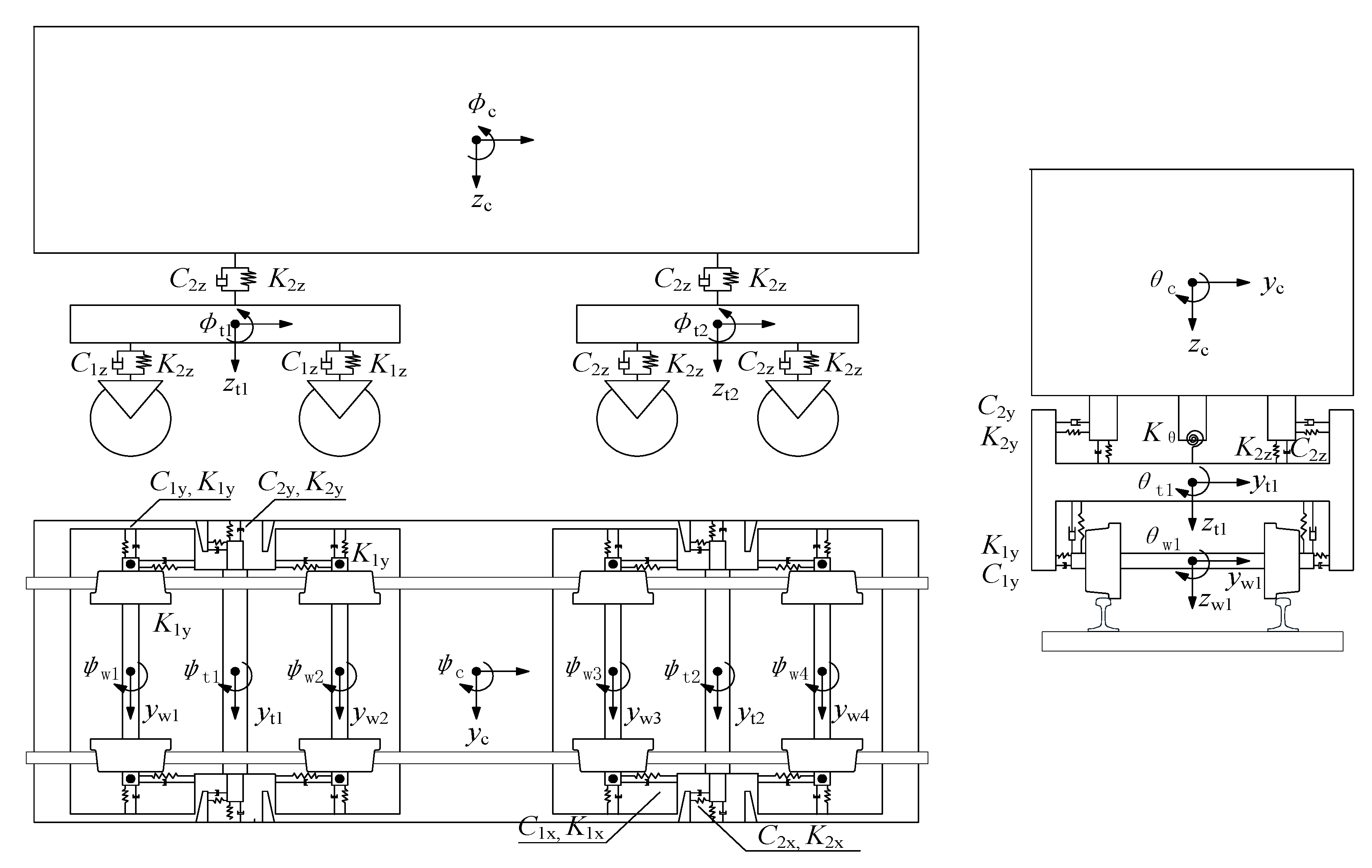
2.1. Establishment of Simulation Model

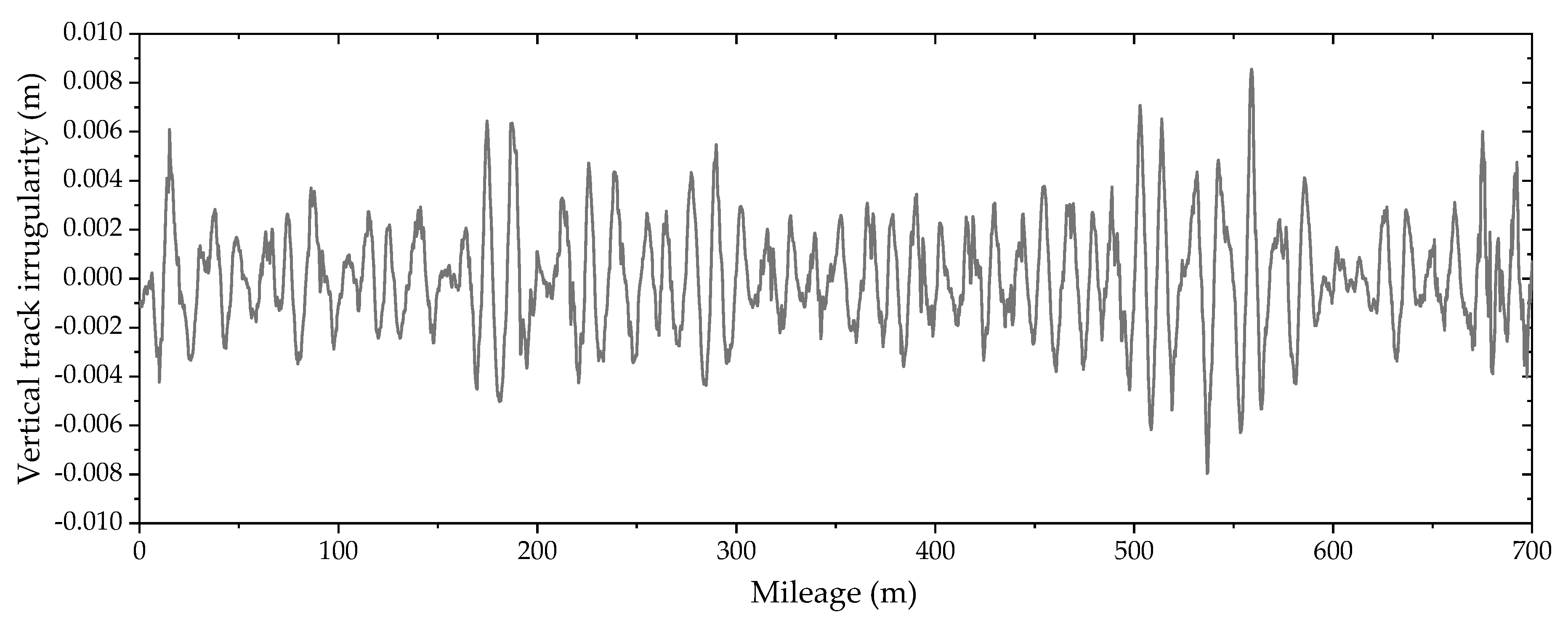
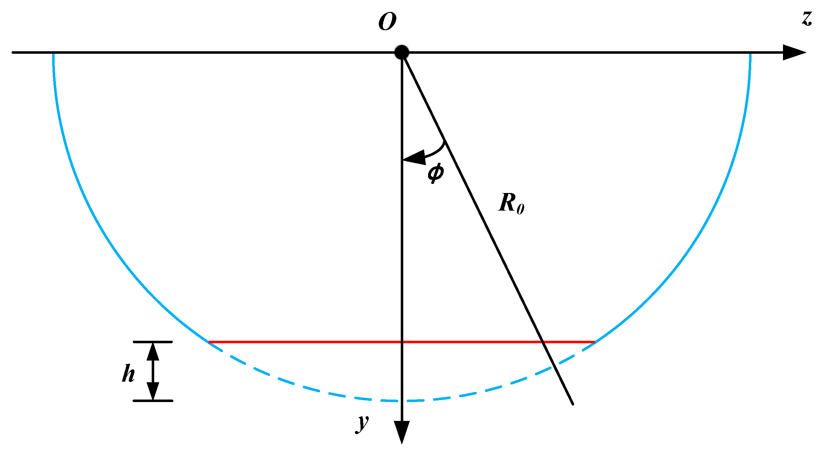
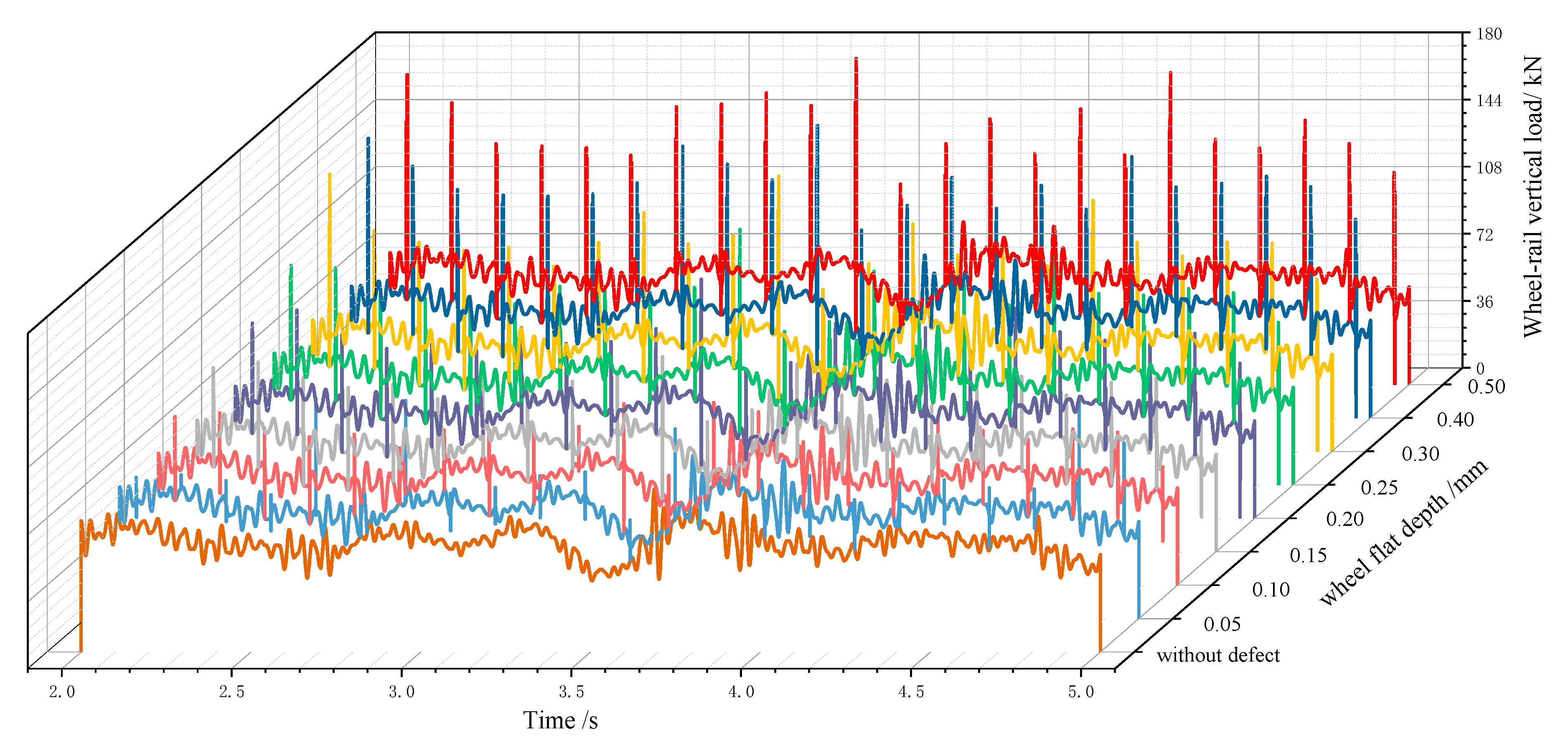
2.1.1. Wheel-Rail Force Simulation Model

Multibody dynamics (MBD) is the science that studies the laws of motion for a multibody system, which is generally composed of several flexible or rigid objects connected to each other. MBD simulation has been widely used in the design, homologation test, and research of railway transportation [26]. The MBD software, Simpack, was used to calculate the wheel-rail forces under different wheel flat conditions. As is shown in Figure 1, the vehicle model had 38 degrees of freedom and consisted of a vehicle body, two bogies, and four wheelsets. The modeling parameters are shown in

Table 1. Parameters of the vehicle model.

Type	Parameter	Value	Unit
Mass	Vehicle body	33,593	kg
	Bogie	3730	kg
	Wheel	1730	kg
Moment of inertia	Vehicle body (around x/y/z axis)	50,000/1,101,000/1,099,000	kg·m2
	Bogie (around x/y/z axis)	1194/876/2099	kg·m2
	Wheel (around x/y/z axis)	1042/137/1042	kg·m2
Stiffness	Primary suspension (longitudinal/lateral/vertical)	17.62 × 106/9.62 × 106/5.35 × 106	N/m
	Secondary suspension (longitudinal/lateral/vertical)	0.16 × 106/0.16 × 106/0.35 × 106	N/m
Damping	Secondary suspension (lateral)	5000	N·s/m
	Secondary suspension (vertical)	5000	N·s/m

.

In actual conditions, the rails are not perfect, which also affects the wheel-rail forces. Therefore, we used a sample of vertical track irregularity measured on a subway in Nanjing, China as the initial excitation of the wheel-rail contact. As shown in Figure 2, the total length of the sample is 700 m and the interval is 0.25 m.

The wheel flats are simulated by defining the deviation of wheel radius. As shown in Figure 3, the equation of the undamaged wheel (plotted in blue) is expressed as follows:

$$z^2+y^2=R_0{}^2$$

(1)

where z and y are the longitudinal and vertical position of a certain point relative to the center of the wheel and $R_0$ is the nominal radius of a perfect wheel.

According to the generation mechanism, a wheel with flats is approximately equivalent to cutting a plane from a certain position on the wheel tread [27]. Therefore, the equation of the flat (plotted in red) can be expressed as follows:

$${y=R}_0-h$$

(2)

where h is the depth of the wheel flat. Convert the above equations into polar coordinates, thus the deviation of wheel radius of a damaged wheel can be expressed as follows:

$$\Delta R\left(\phi \right)=\{\begin{array}{c}0,\phi \ge \frac{{\alpha }_R}{2}\mathrm{or}\phi \le -\frac{{\alpha }_R}{2}\\ R_0-\left|\frac{R_0-h}{\cos \left(\phi \right)}\right|,-\frac{{\alpha }_R}{2}<\phi <\frac{{\alpha }_R}{2}\end{array}$$

(3)

where $\phi$ is the angle between the radial line and the vertical line through the center of the wheel, ${\alpha }_R$ is central angle corresponding to the wheel flat region and equals ${2\times \cos }^{-1}{\left[\right(R}_0{-h)/R}_0]$.

By defining the radius deviation of wheels according to Equation (3), the geometric information of the wheel flats is input into the Simpack model. In this section, we have set nine damage conditions of different flat depths from 0 to 0.5 mm. Only one of the eight wheels has wheel flat and the vehicle runs at a speed of 20 m/s with a sampling frequency of 4 kHz. The calculated wheel-rail forces of different damage conditions are shown in Figure 4. The occurrence of wheel flats induces intermittent peaks to the load history and the amplitude increases as the depth grows.

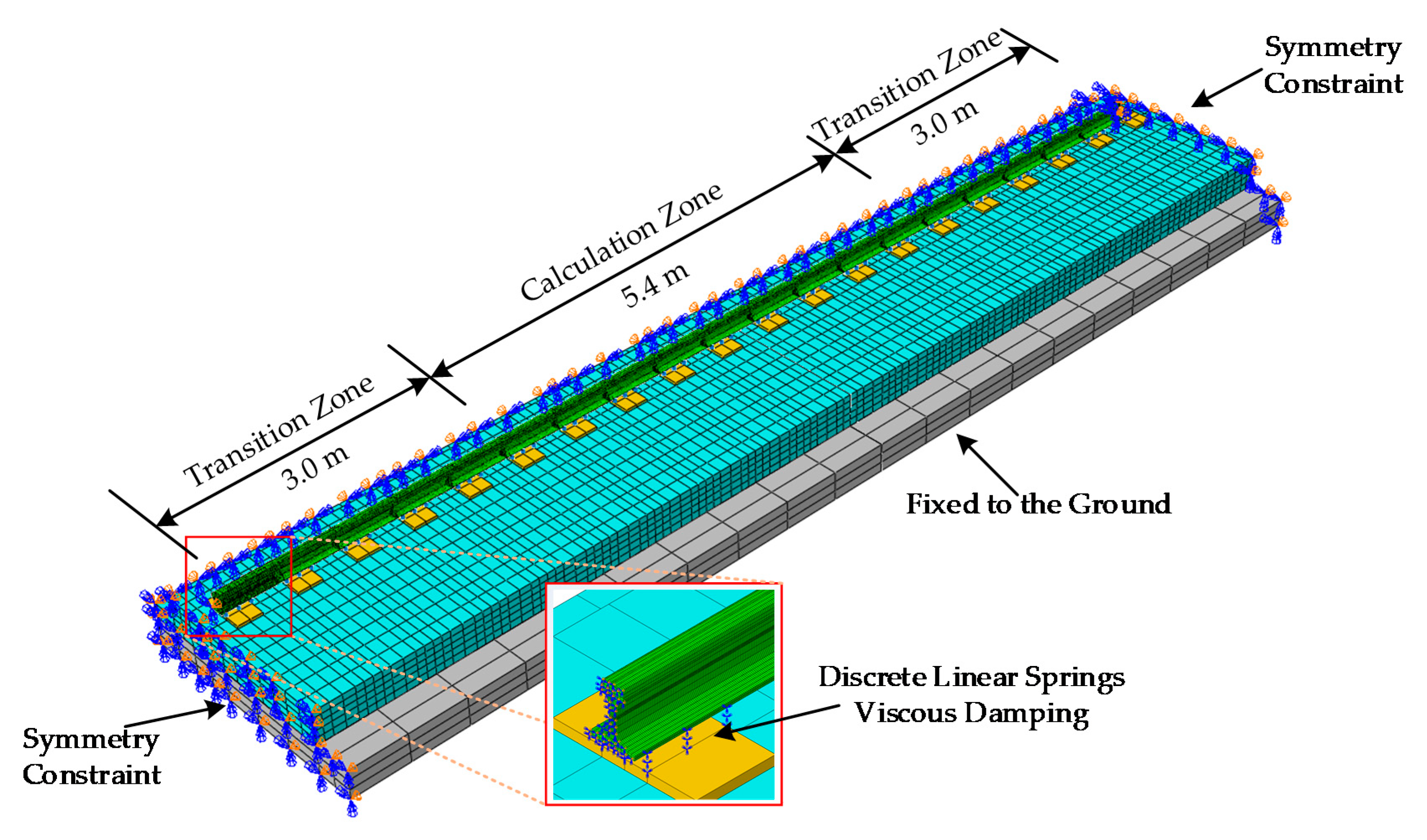
2.1.2. Refined Rail Response Simulation Model

A refined numerical model (shown in Figure 5) is developed with finite element method (FEM) software Abaqus to investigate the strain responses of rails under the previous calculated wheel-rail forces. The rails, sleepers, and slab track are modeled with solid elements according to their respective nominal geometry and material properties. The fastener system is modeled with multiple discrete linear springs and viscous damping to simulate the effect of rail pads and clamps.

The boundary settings are shown in the picture. To avoid the influence of boundary conditions on the calculation results, the model is divided into a calculation zone and two transition zones. The rail in the calculation zone is more precisely meshed. The mesh size in the longitudinal direction is 5 mm because the per unit time movement of the load on the rail is 5 mm at the given sampling frequency of 4 kHz. Since the sensors are usually mounted at the rail web or near the rail foot, due to the limitation of installation condition, the meshes at these regions are refined in the cross-section.

To transmit the wheel-rail forces to the FEM model, the user subroutine VDLOAD of Abaqus is deployed. The role of this subroutine is to define nonuniformly distributed loads as a function of position, time, and velocity, etc. According to the Hertz contact theory [28], the elastic deformation of the steel of the wheel and the rail creates an elliptic contact area. Assuming that the contact elliptic does not change during the movement, the effect of the vehicle can be regarded as a moving surface load applied to the tread of the rail. In the VDLOAD, the contact elliptic is simplified to a rectangular area (15 mm × 5 mm). The velocity of the moving load is 20 m/s and the load history are specified by the former section. The steps of the VDLOAD, at each point in time, are as follows: (1) Determine the center position of the load based on the speed of the vehicle and the time of the movement, (2) determine the contact area according to the predefined contact elliptic size, and (3) traverse all the nodes on the rail tread and calculate the stresses exerting on the nodes within the contact area in accordance with the load history.

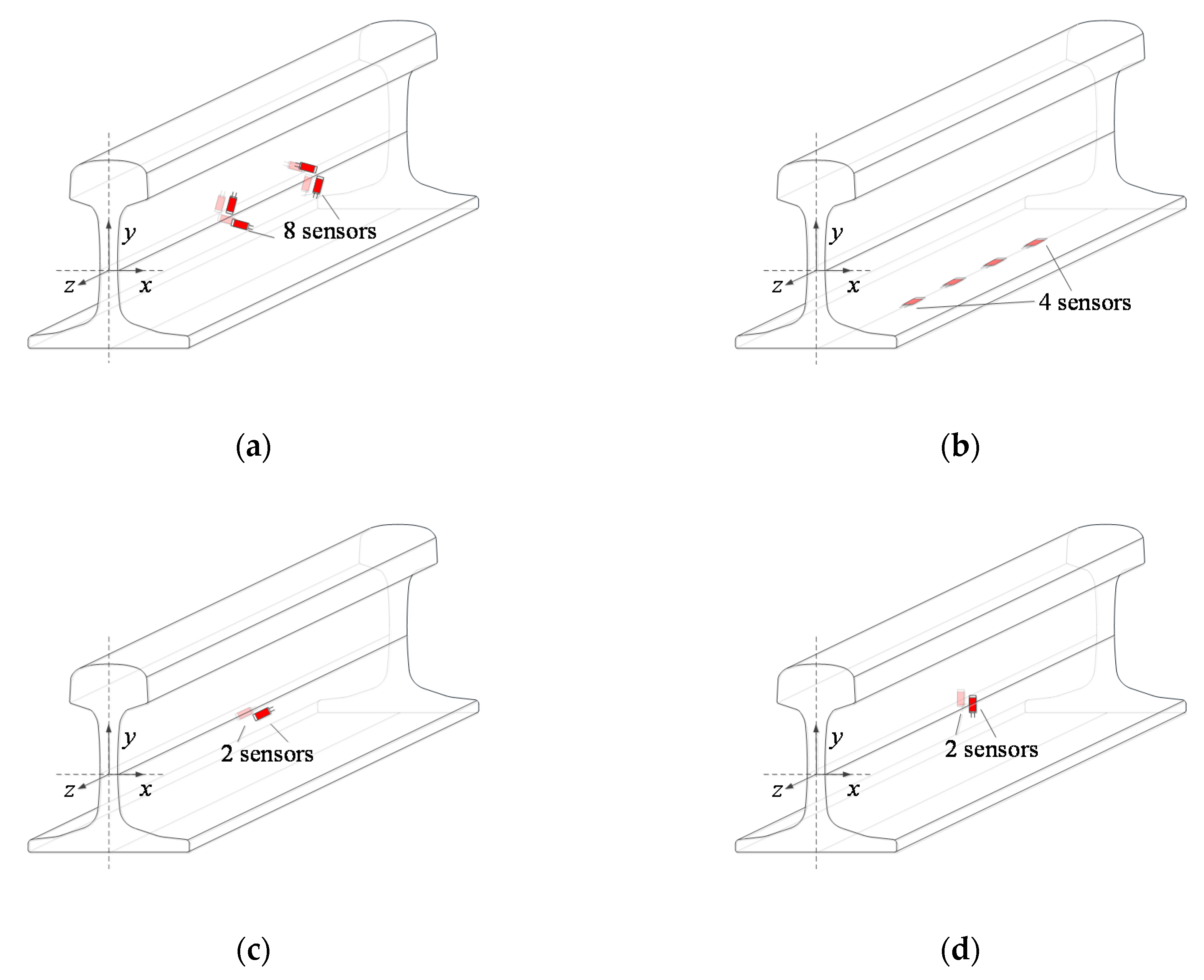
2.2. Layout Scheme of Multisensor Arrays in the Rail Cross-Section

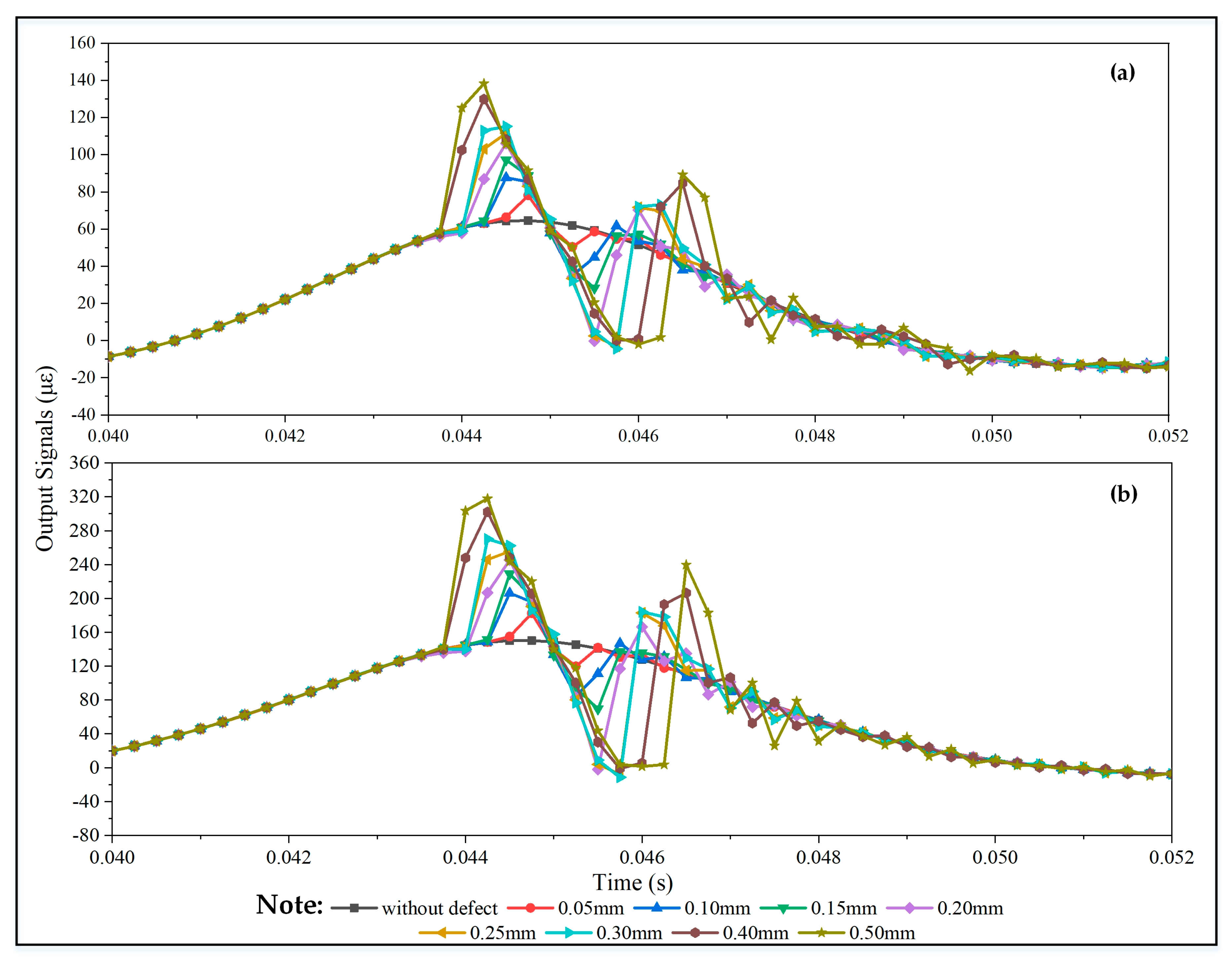
2.2.1. Sensitivity of Different Layout Schemes to Wheel Flats

Considering that the vertical rail responses surge intensively when wheel flats exist [29], measurement methods for vertical wheel-rail forces are feasible solutions to monitor the wheel defects. Conventional vertical wheel-rail forces measurement methods include: (1) sheer force method [30], (2) rail base bending moment method [31], (3) rail web bending moment method [32], and (4) rail web compression method [33]. Although they have different layout schemes (shown in Figure 6), they all achieve the purpose by establishing a relationship between the sensor outputs and the vertical loads.

Although the sheer force method is widely used in field tests for wheel-rail force, it is not a suitable choice for the long-term monitoring of wheel flats because this method uses eight strain gauges to form a bridge which is vulnerable to water and electromagnetic environment. In addition, the baseline drift is inevitable for strain gauges during long-term service, making it impossible to stay consistent for a long period of time. The rail base bending moment method is not an ideal choice since all the sensors are required to be attached to the bottom of the rail along the longitudinal direction which makes it difficult to ensure the installation accuracy without replacing the rail.

In contrast, the latter two methods, rail web bending moment and rail web compression, seem to have more potential for the long-term monitoring of wheel flats. For these methods, only two sensors need to be installed at the rail web. It is worth mentioning that the aim of this study is the recognition of wheel defects. Therefore, the sensors mounted on rails should capture the abnormal impact signals excited by wheel flats as effective as possible, rather than measure the exact dynamic loads. In view of this, we analyzed the sensitivity of these two methods under different defect conditions using the established refined rail response model. The predefined defect depths varied from 0 to 0.5 mm.

As illustrated in Figure 7, the output signals of these two methods have similar characteristics. Each series of signals consists of a major trend reflecting the wheel passage, as well as the fluctuation induced by a wheel flat. As the depth of the wheel flat increases, the fluctuation becomes more intense.

It is obvious that signals collected by the rail web compression method are much stronger than those of its counterpart. Therefore, the rail web compression method is considered to be more sensitive to wheel flat impact because the signals collected by the rail web bending moment method are essentially the longitudinal dynamic bending strains caused by the wheel loads. Since the sensors are mounted near the neutral axis, the strains are relatively small. By adjusting the sensor positions away from the neutral axis, the test results are further improved. It is, nevertheless, inevitable that the installation of sensors is hindered by track equipment such as fasteners and sleepers.

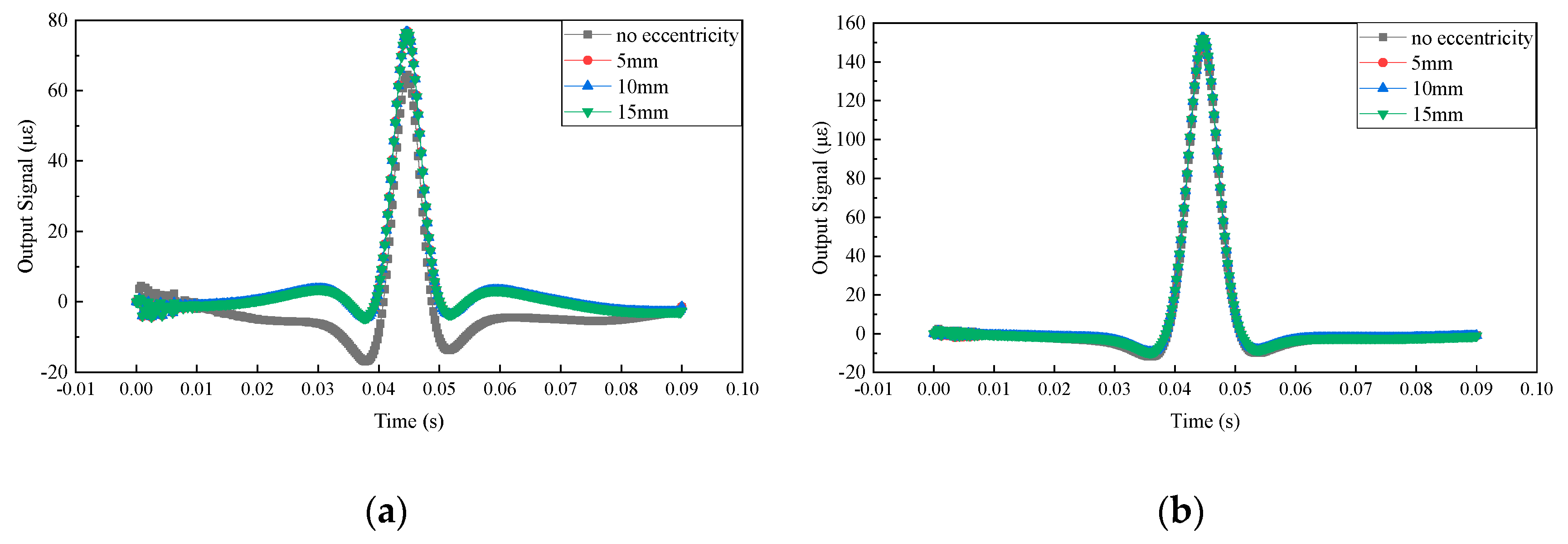
2.2.2. Influences of Wheel-Rail Contact States on Different Layout Schemes

In addition to the vertical wheel loads, the rail is also subjected to bending moments and torques caused by the lateral wheel-rail forces and wheel eccentricity which makes the strain distribution in the rail cross-section much more complicated. Therefore, the selected method is supposed to be immune to these interferences, and therefore is better able to capture the vertical impacts caused by wheel flats.

To determine the influences of lateral forces, the model established in Section 2.1 was used to simulate the outputs of different sensor layout schemes during an intact wheel passage. Different levels of lateral forces (0, 10, 20, 30, and 40 kN) were exerted to the model during the process. Figure 8 shows the effects of the different lateral forces on the outputs of the rail web bending moment method and the rail web compression method. We concluded that the existence of lateral forces plays an important role in the measurement of the rail web bending moment method, while on the contrary, it has little effects on the test results of the rail web compression method.

Similarly, we analyzed the influences of wheel eccentricity on different layout schemes. In the analysis, wheel eccentricity is defined as the distance between the wheel-rail contact center and the symmetry axis of the rail. Figure 9 shows a comparison of the output signals of these two methods under different wheel eccentricity conditions (0, 5, 10, and 15 mm). Apparently, wheel eccentricity has a greater impact on the rail web bending moment method.

Figure 10 concludes the influences of different wheel-rail contact states on these two layout schemes. The Y-axis represents the errors under different interferences. The result shows that the rail web compression method is the optimal solution for the sensor layout in the rail cross-section.

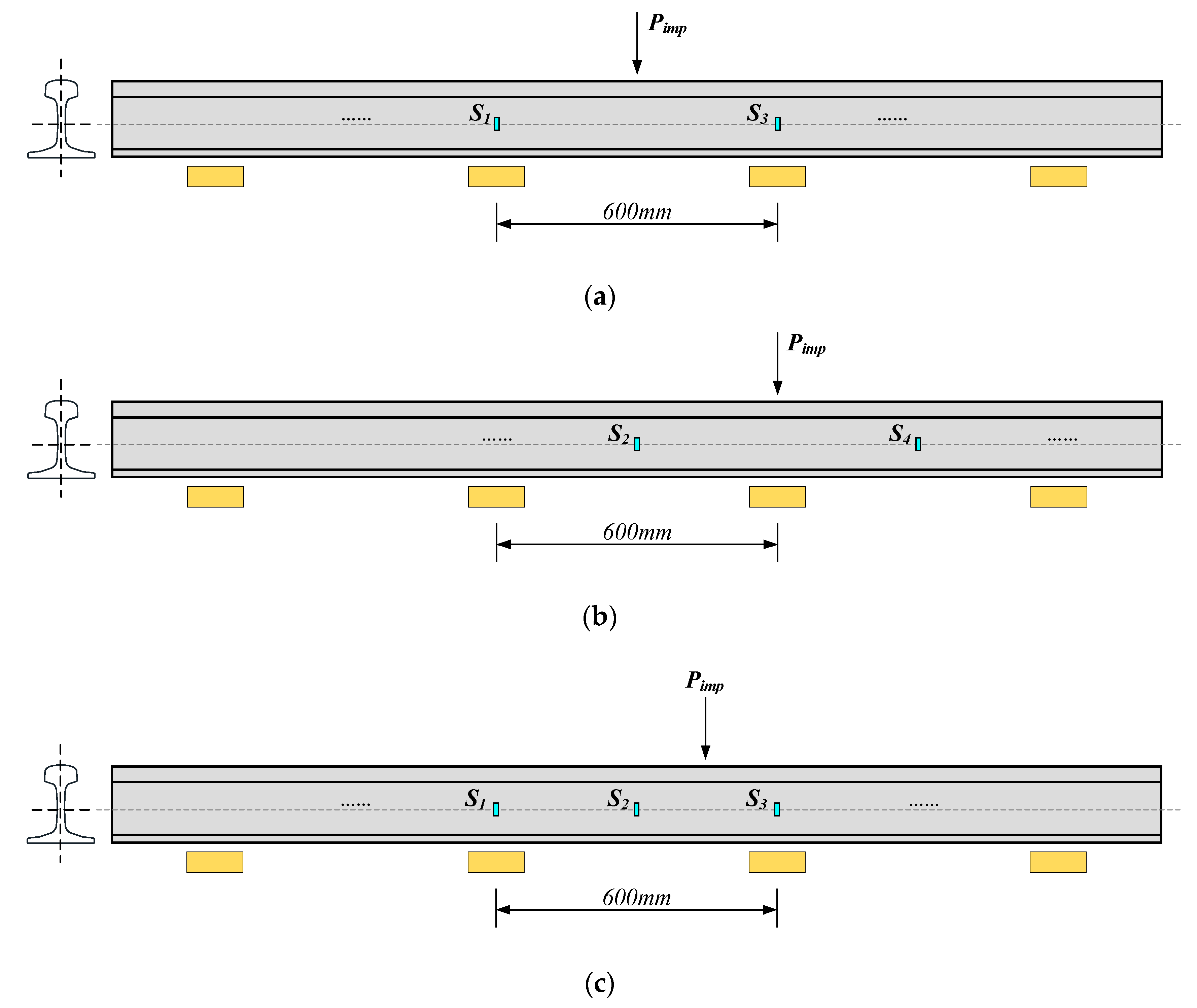
2.3. Layout Scheme of Multisensor Arrays along the Longitudinal Direction of Rail

2.3.1. Design of Sensor Arrangement Spacing in the Longitudinal Direction

In order to ensure that the multisensor arrays effectively capture the impact signals caused by wheel defects and avoids omissions, it is necessary to find out a reasonable spacing arrangement of sensors. Considering the limited spaces for railway field monitoring, three layout schemes for multisensor arrays in the longitudinal direction are proposed, as shown in Figure 11. Although other positions also have potential for the sensor arrangement, they are not discussed in this section because they are not easy to locate during installation.

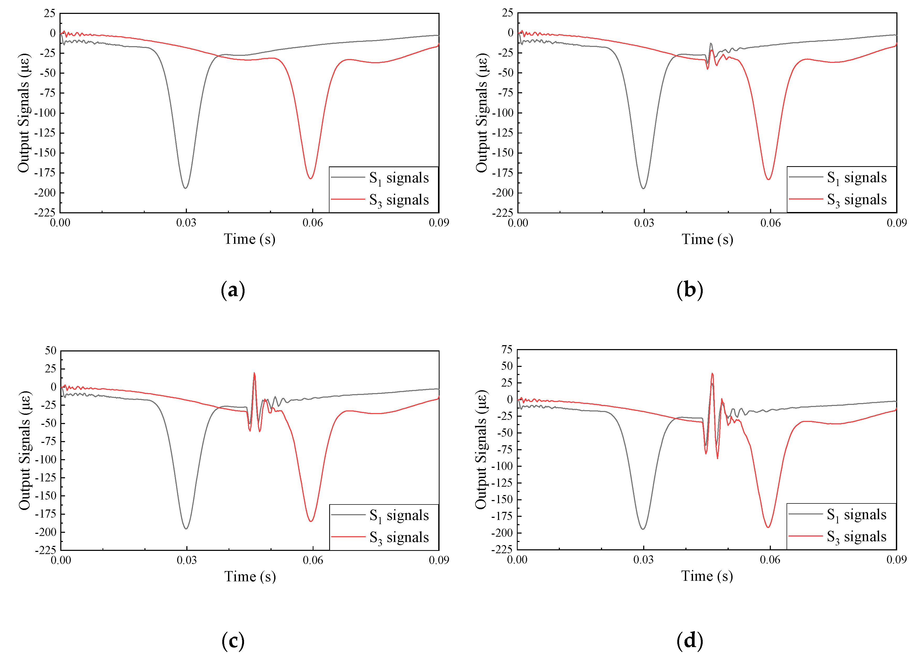
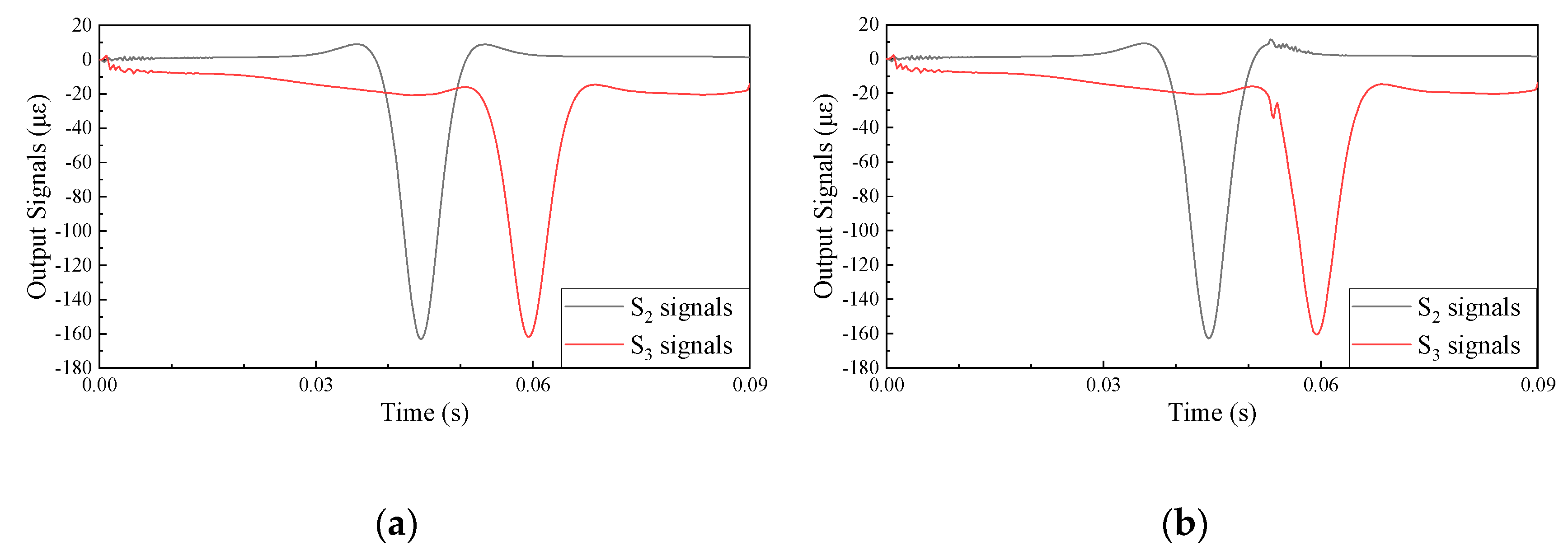
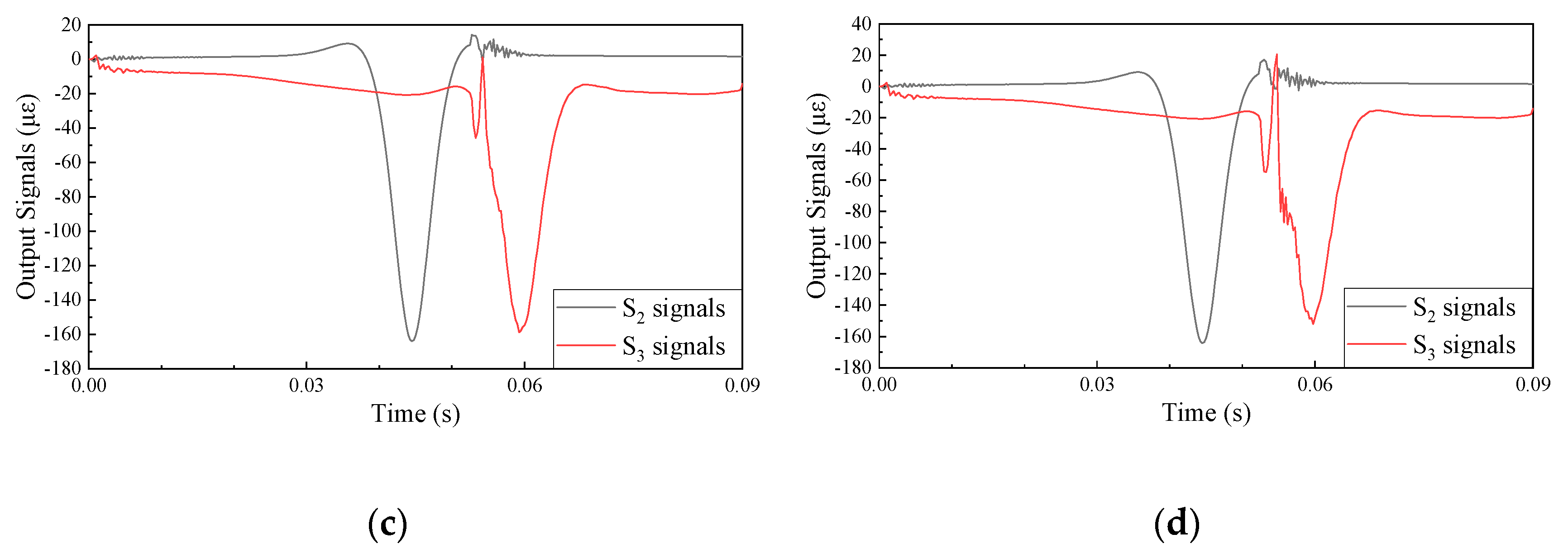
2.3.2. Comparison of Different Sensor Arrangement Plans

The “most unfavorable impact position” is introduced to describe the impact position which is most difficult for adjacent sensors to recognize. The most unfavorable impact position is generally the middle position between every two sensors. When the wheel flat hits exactly this position, the impact signals collected by sensors are weakest.

The most unfavorable impact positions of the above plans are marked with P_imp. By adjusting the initial time of the simulation, the wheel flat impacts are ensured to occur just at those most unfavorable positions. Figure 12 shows the output signals of Plan I, where wheel flat impact occurs in the middle of the sleeper spacing. The wheel flat causes a sudden change in the signals of both adjacent sensors. Even when the wheel defect is very slight, for example, 0.1 mm, the sensors still completely capture the abnormal responses. As the depth increases, the sudden change becomes more intense.

Figure 13 shows the output signals of Plan II where the wheel flat impact occurs right above the sleeper. Compared to Plan I, the signals of Plan II are much weaker, even if the wheel flat depth reaches 0.5 mm. When applied to the field test, the impact signals are likely to be submerged in system noises.

Plan III is essentially a combination of Plan I and Plan II. As shown in Figure 14, although the distance between sensors is halved, the test effects are not necessarily improved. Contrarily, the output signals are very dissimilar because the sensors are mounted in two different situations. In the middle of the sleeper spacing, the rail is relatively free in the vertical direction. Most of the wheel flat impact energy is dissipated through the vertical rigid body motion of the rail, leading to the smaller compression strain at the rail web. Therefore, the responses of sensors installed in these locations, like S₂, are much weaker. Whereas for the rail above the sleepers, it cannot freely vibrate because of the restraints of sleepers. The impact energy is mostly converted into elastic potential energy of the rail. As a result, these sensors, like S₃, have stronger output signals.

However, the fusion of multiple sensors is reliable only when the sensors are mounted in identical situations. Otherwise, the adjacent sensors have different transfer functions to the same excitation. This means that signals sampled by sensors are based on different baselines. Therefore, Plan III is not suitable for the sensor arrangement. By comparison, Plan I is considered as the best option.

3. Wheel Flat Recognition and Positioning Algorithm Based on Multisensor Arrays

3.1. Design of the Algorithm

Using the established models, we simulated the output signals of the multisensor arrays during a bogie passage. Figure 15a shows the movement of the defected bogie and the configuration of the sensors. There is a wheel flat with a depth of 0.2 mm at the front wheel, whereas the rear wheel is intact. Ten pairs of sensors are mounted on the rail web, marked from S₁ to S₁₀. The length of a multisensor array is 5.4 m, which is longer than the circumference of the wheel. Thus, every wheel revolves two times during its passage of the measurement area. This ensures that a flat spot on the wheel hits at the rail tread within this segment no less than two times. Figure 15a shows the output signals of S₄. The successive two troughs represent the respective moments when the front and rear wheels arrive at the location of S₄. Similarly, Figure 15b,c displays the outputs of S₅ and S₆. We found that the outputs of different sensors have almost the identical main trend, except for the time delay due to the arrangement of sensors.

Apparently, the defected front wheel significantly influences the outputs of sensors. There are two obvious impact processes sensed by all the sensors. At 0.21 s, the defected wheel exactly hits the rail above S₅. Therefore, the fluctuation amplitude of S₅ at this moment is much greater than those of S₄ and S₆. With the rotation of the wheels, the flat spot on the front wheel hits the rail again between S₉ and S₁₀, at 0.34 s. However, this time the fluctuation caused by the impact process occurs just around the second trough of S₆ that reflects the arrival of the rear wheel. The reason is that the rear wheel is above S₆ at this moment. If we only observe the outputs of S₆, it is easy to draw the wrong conclusion that the rear wheel is also damaged.

Since the in situ condition is much more complex than this case (the only imperfectness is a flat spot on the front wheel), separate analysis can hardly acquire the accurate information. Even if we observe the responses of multiple sensors on the same wheel, it is still difficult to have a comprehensive understanding of the wheel states. Therefore, data fusion of multiple sensors is critical to the better diagnosis of wheel defects. On the basis of the correlations between sensors, we designed a wheel flat recognition and positioning algorithm. As shown in Figure 16, by solving the three key problems of “when”, “where”, and “which wheel”, successively, it accurately accesses the damage states of the wheels.

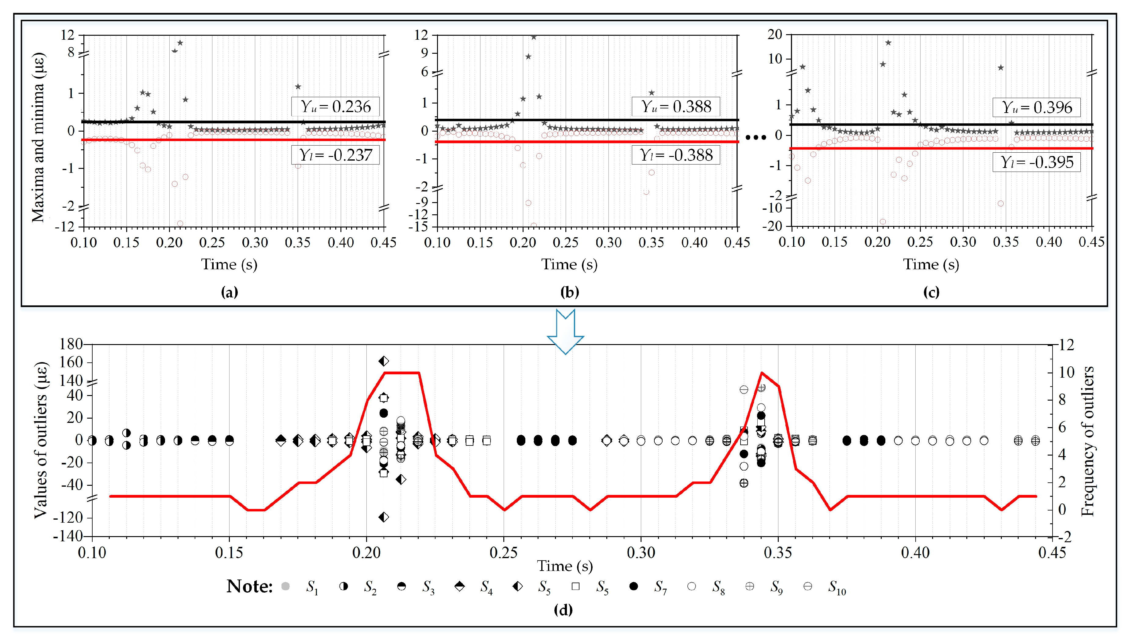
3.2. Step I: When the Abnormal Impacts Occurred

The purpose of this step is to determine the specific moments when abnormal impacts occur. The fast Fourier transform (FFT) filter is applied to eliminate the major trends of output signals. With a cut-off frequency of 200 Hz, the high-frequency components caused by wheel flats are extracted, as shown in Figure 17. After the high-pass filtering, the defect signals become much more obvious. All 10 sensors have sensed two anomalous responses caused by the wheel flat on the front wheel at 0.21 s and 0.34 s.

Additionally, an interesting fact is that the response amplitudes of sensors to a certain wheel flat seem to obey some special distribution. As the red dashed lines show, the responses to the first impact are almost symmetrically distributed around the location of S₆. As for the second impact, the amplitude of response increases along with an increase of the sensor’s sequence number. This characteristic provides a hint as to how to locate where the impact happens, which will be later discussed in the Section 3.3.

In order to screen out all the impact processes, the sliding window method is introduced in this step. As is shown in Figure 17, the sliding window, with a size of d, moves forward progressively by the step length of δ. The window is a matrix containing the signals of multiple sensors in a certain time range, which can be expressed as follows:

$$W_k=\left(\begin{array}{ccccc}{S}_1,N_k& S_1,N_k+1& \dots & S_1,N_k+M-2& S_1,N_k+M-1\\ S_2,N_k& S_2,N_k+1& \dots & S_2,N_k+M-2& S_2,N_k+M-1\\ ⋮& ⋮& \ddots & ⋮& ⋮\\ S_{N_s-1},N_k& S_{N_s-1},N_k+1& \dots & S_{N_s-1},N_k+M-2& S_{N_s-1},N_k+M-1\\ S_{N_s},N_k& S_{N_s},N_k+1& \dots & S_{N_s},N_k+M-2& S_{N_s},N_k+M-1\end{array}\right)$$

(4)

where N_s is the number of sensors. In this case, N_s = 10. M is the number of samples of each step determined by the window size d and the sampling frequency f. N_k represents the starting number of the sample in the k-th step. These two parameters can be calculated using the following equations:

$$M=d\times f$$

(5)

$$N_k=1+(k-1)\times \delta \times f$$

(6)

Outlier tests are performed during every step. Since the filtered signals are not normally distributed, the boxplot method is deployed to distinguish the outliers. This method uses quantiles to determine the thresholds of the normal data, which can effectively eliminate the influence of extreme values on the overall distribution. In light of this, the boxplot method has strong robustness in the outlier test for non-normally distributed data.

The upper and lower thresholds of the normal signals of i-th sensor specified by the boxplot method can be expressed in Equations (7) and (8), respectively [34].

$$Y_u{=Q}_3+\alpha \times IQR$$

(7)

$$Y_l{=Q}_1-\alpha \times IQR$$

(8)

where $Q_3$ and $Q_1$ are the upper and lower quartiles of the sample, $IQR$ is difference between $Q_3$ and $Q_1$, and $\alpha$ is an adjustable coefficient which is often set as 1.5. Outliers are defined as values outside the range between $Y_u$ and $Y_l$.

By comparing the maxima and minima of every row of W_k with the calculated thresholds, we discover how many sensors have sensed some abnormal fluctuations in the corresponding time range. Figure 18a illustrates the maxima and minima of the sensor S₁ during every sliding step. The black dots represent the maximums and the red ones stand for the minimums. Compared with $Y_u$ and $Y_l$ (black and red solid lines), outliers of S₁ during the measurement can be screened out. Similarly, the outliers of other sensors are shown in Figure 18b,c.

The outliers collected from the sliding window method are drawn in Figure 18d. It can be seen that all the outliers are clustered at two moments. To eliminate the interferences of sensor noises, the frequency of outliers in every step is calculated and shown with the red curve. If there are more than five sensors that have outliers in a certain step, the corresponding period is regarded as an impact process. These periods are denoted as time series IMP_j (j = 1, 2, …, N_I) where N_I is the number of identified impact processes. In this case, two impact processes have been screened out through the sliding window method, i.e., IMP₁ (0.1875~0.225 s) and IMP₂ (0.325~0.35 s).

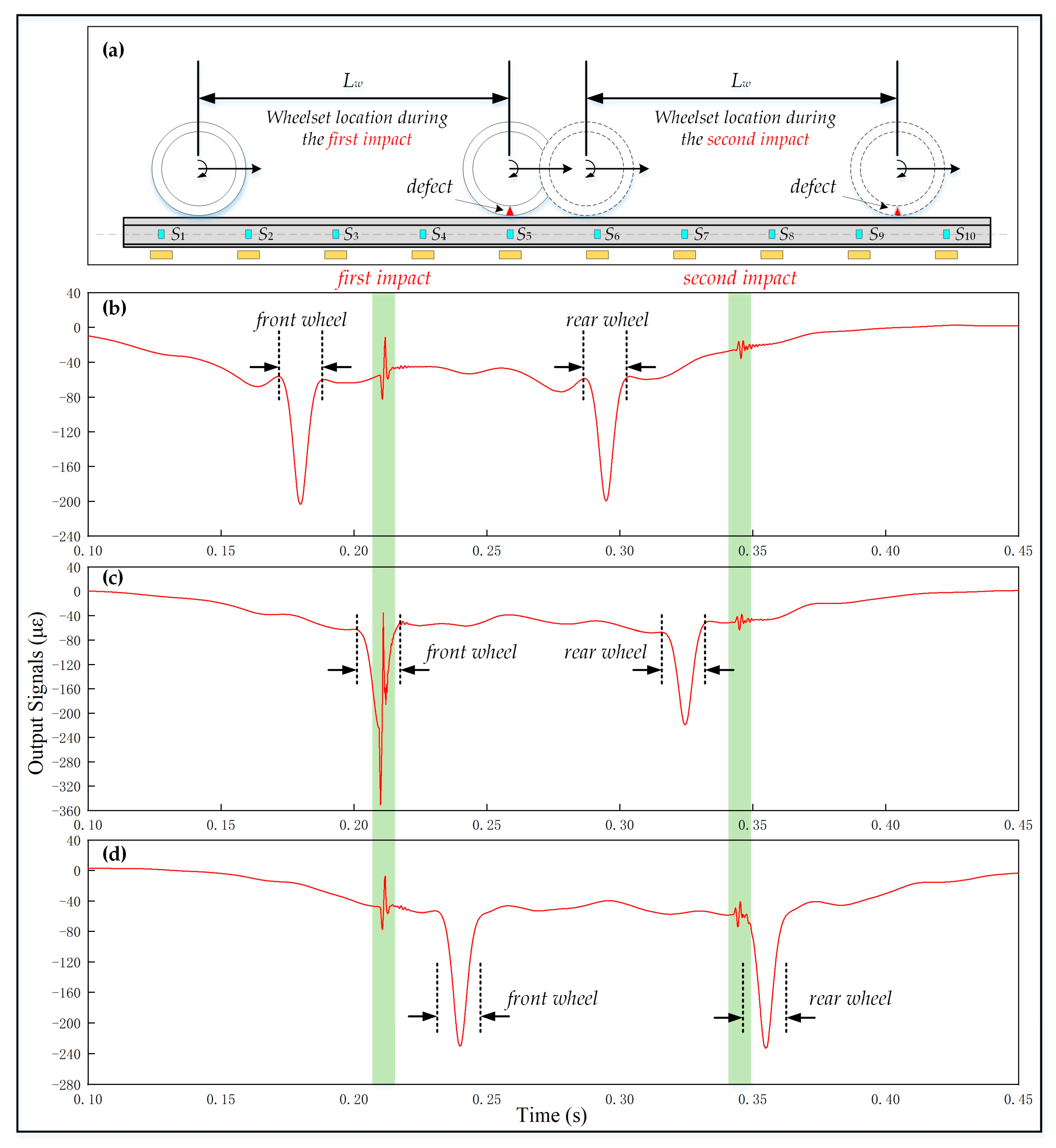
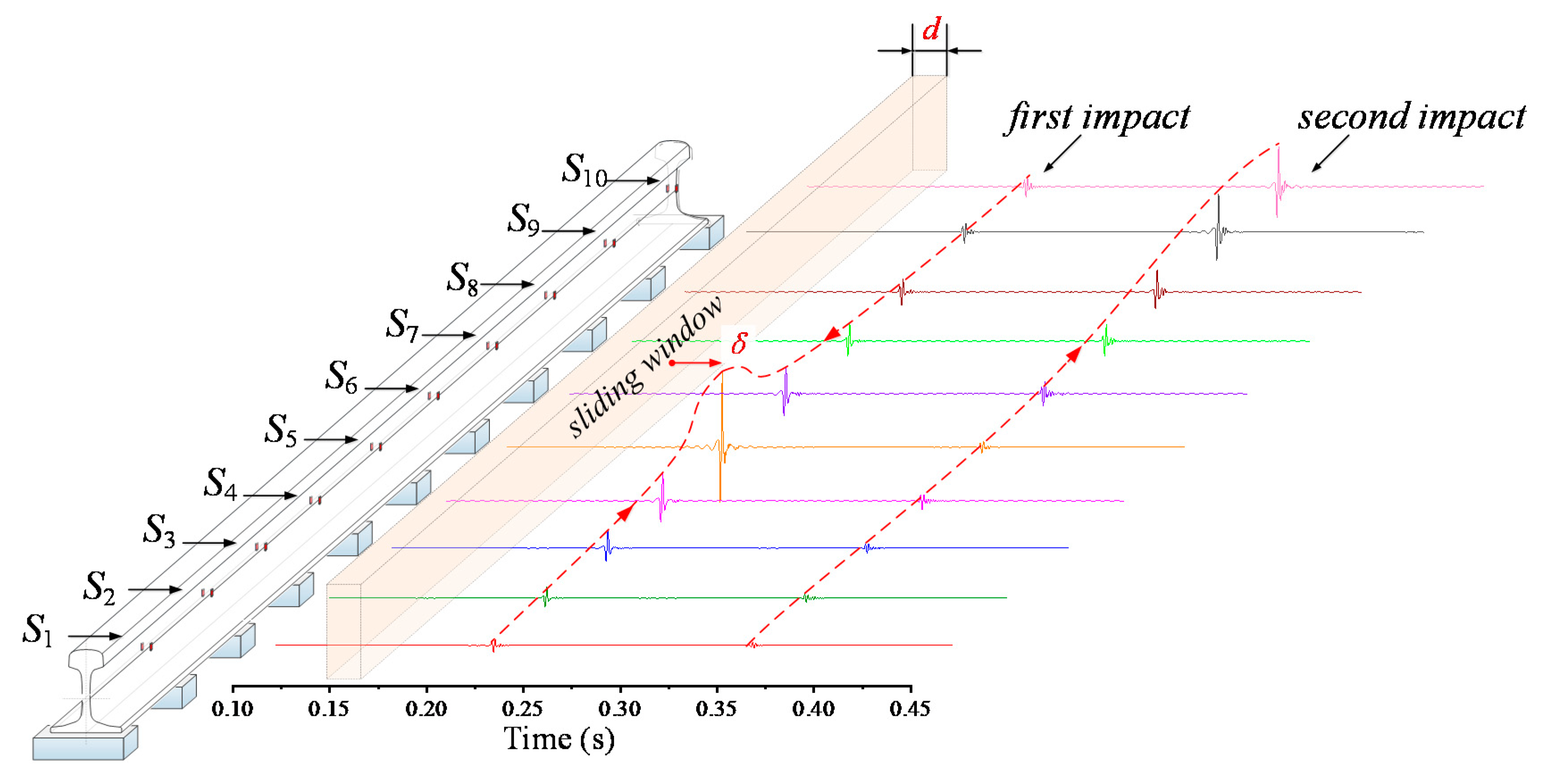
3.3. Step II: Where the Abnormal Impacts Occurred

The purpose of this step is to position the specific location of each abnormal impact. For every impact process identified in Section 3.2, the filtered signals during the corresponding period are extracted and arranged in order, according to the positional relationship of sensors. This gives us a different perspective, i.e., as if observing Figure 17 from the right side.

We found that there is an obvious correlation between the amplitudes and the impact location. Figure 19b illustrates the filtered signals of all sensors during IMP₁. During this process, the impact location is just over S₅, leading to the much higher output of S₅ than its counterparts. A similar conclusion can also be drawn according to Figure 19c.

Inspired by this, a data sequence containing the maximum values of every sensor’s outputs during IMP_j is acquired as follows:

$${Ex}_j={\left({Max}_{j,1}{,Max}_{j,2},\cdots {,Max}_{{j,N}_s}\right)}^T$$

(9)

where Max_j,i (i = 1, 2, …, N_s) is the maxima of the sensor S_i’s outputs during IMP_j.

To better describe, a parameter, namely “flag”, is introduced to represent the impact location. As is shown in Figure 19a, the value of flag is set as 1.5 in the beginning. All the elements of ${Ex}_j$ are compared successively to determine the impact location. If Max_j,i+1 is greater than Max_j,i, then, the value of flag is increased by one, meaning that the impact is supposed to occur somewhere behind S_i. On the contrary, if Max_j,i+1 is less than Max_j,i, then the value of flag stays unchanged. After the calculation, the nearest two integers to the parameter flag suggest the location of a certain impact process. For instance, the final value of flag for IMP₂ is 9.5, which means that the most probable location of the second impact process is between S₉ and S₁₀.

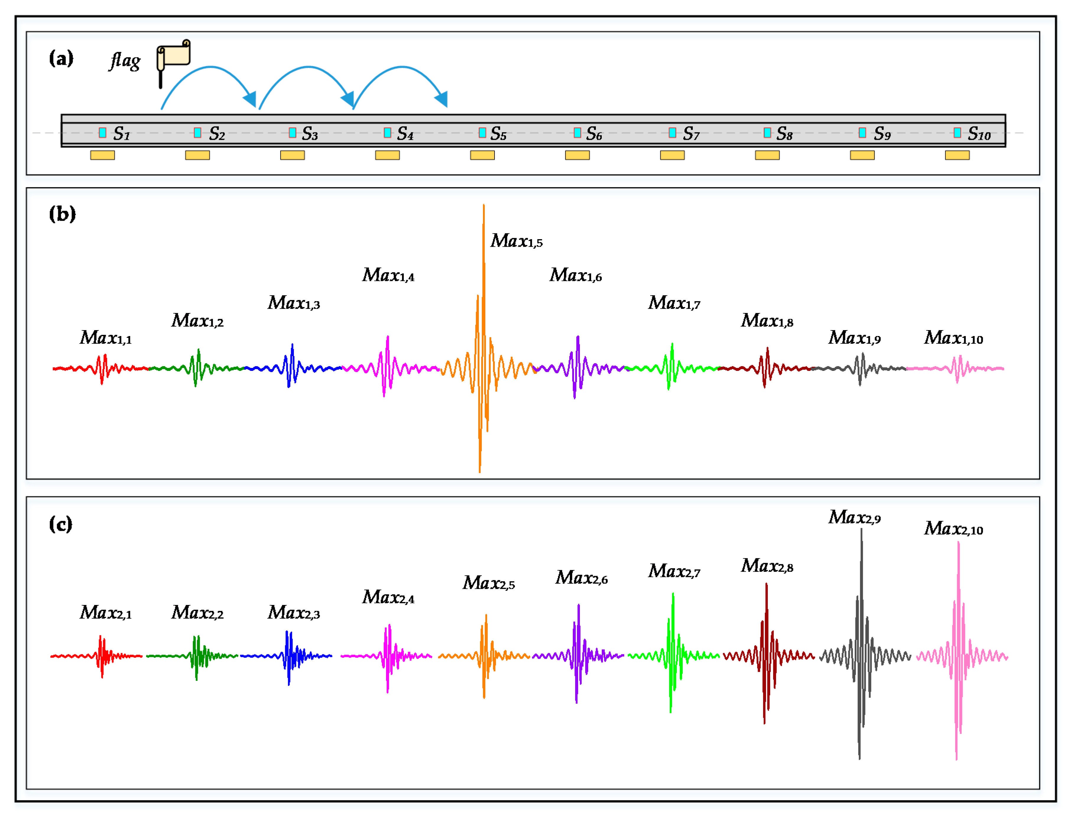
3.4. Step III: Which Wheel is Responsible for the Abnormal Impact

The first target of this step is to calculate the average speed of the wheels. Since the distance between the sensors is fixed once installed, the average speed of the wheels can be obtained by calculating the sensor spacing divided by the interval of troughs. The average speed of the wheels is denoted as $v_w$.

Indeed, there can only be one wheel at a specific time and position. Therefore, as long as the positions of the wheels are determined, it is possible to find out the source of impacts. The position of S₁ is regarded as the origin of the coordinate. The time when the front and rear wheels arrive at the origin are denoted as $t_{ini,front}$ and $t_{ini,rear}$. For the j-th (j = 1, 2, …, N_I) impact process, the locations of the front and rear wheels can be described by the following equations, respectively:

$$S_{j,front}=v_w\times (t_{j,imp}-t_{ini,front})$$

(10)

$$S_{j,rear}=v_w\times (t_{j,imp}-t_{ini,rear})$$

(11)

where $t_{j,imp}$ is the middle time of the j-th impact process IMP_j.

According to the above method, the following result is obtained: During IMP₁ (0.1878~0.225 s), the front wheel is between S₅ and S₆, while the rear wheel is between S₂ and S₃. During IMP₂ (0.325~0.35 s), the front wheel is between S₁₀ and S₁₁, while the rear wheel is between S₆ and S₇. According to the impact positions detected in Section 3.3, all the impact processes are identified as being generated by the front wheel, which is consistent with the predefined condition.

4. Validation of the Algorithm

Validation of the recognition and positioning algorithm was conducted via the experimental method. The offline wheel condition inspection was conducted to measure the radius deviation of the wheels. After several repeats of the experiments, two wheels with relatively severe wheel flats were chosen for the algorithm validation. Figure 20 shows the defect conditions of these two wheels. More specifically, there are two obvious wheel flats with approximate depths of 0.06 mm and 0.04 mm on the front wheel, and one wheel flat with an approximate depth of 0.07 mm on the rear wheel. The measured wheel profiles were input into the simulation model as the front and rear wheels, respectively. The sensor layout is consistent with Section 3.

To consider the influence of the monitoring system error, a 5% (SNR = 13 dB) Gaussian noise is added to the calculated output signals. Figure 21 shows the results of the simulation. For easier observation, the baselines of signals are shifted to different degrees. The abnormal data caused by multiple wheel defects mingles together, making it impossible to assess the real conditions of the wheels directly.

The algorithm proposed in Section 3 was used to identify the defect conditions of the wheels. The curves in Figure 22 illustrate the filtered signals and identified impact processes, while the histogram represents the frequency of outliers during every time step. The results show that there are 8 periods of time identified as potential impact processes. They are denoted as IMP₁ (0.1125~0.11875 s), IMP₂ (0.15625~0.1625 s), IMP₃ (0.18125~0.1875 s), IMP₄ (0.24375~0.25 s), IMP₅ (0.2875~0.29375 s), IMP₆ (0.30625~0.3125 s), IMP₇ (0.38125~0.3875 s), and IMP₈ (0.44375~0.45 s).

Furthermore, the position of every impact process, as well as the locations of the wheels, are determined. The results are concluded in

Table 2. Results of the recognition and positioning algorithm.

Impact Processes	Impact Position	Middle Time/s	Front Wheel Position/m	Rear Wheel Position/m	Responsible Wheel
IMP1	0.6~1.2 m	0.109375	1.1225	−1.1725	Front wheel
IMP2	1.8~2.4 m	0.153125	1.9975	−0.2975	Front wheel
IMP3	0~0.6 m	0.178125	2.4975	0.2025	Rear wheel
IMP4	3.6~4.2 m	0.240625	3.7475	1.4525	Front wheel
IMP5	4.2~4.8 m	0.284375	4.6225	2.3275	Front wheel
IMP6	2.4~3 m	0.303125	4.9975	2.7025	Rear wheel
IMP7	6.4~7 m	0.371875	6.4975	4.2025	Front wheel
IMP8	5.4~6 m	0.440625	7.7475	5.4525	Rear wheel

. The initial time for calculating the locations of the front wheel is 0.0595 s. As for the rear wheel, the initial time is 0.17425 s. The reason for the negative values of the rear wheel position is that the rear wheel has not entered the test area at this moment. It is obvious that five abnormal impact processes are generated by the front wheel, and the others are due to the defects of the rear wheel.

To better describe the defect conditions of the wheels, the abnormal signals are converted into the polar coordinate system, where the responses represent the deviation of the radius. In this way, the wheel conditions can be deduced and illustrated in Figure 23. The impact signals collected by different sensors converge to the same center angle, reflecting that the wheel flat is most likely to be at this position. From the results of the algorithm, it can be deduced that there are two flat spots on the front wheel and one flat spot on the rear wheel, which matches well with the offline inspection results. Therefore, the algorithm is proven capable of effectively capturing the existences of wheel flats.

5. Conclusions

In this paper, the strain distribution characteristics of the rails under different wheel flat conditions were analyzed using the numerical method. On the basis of this, we designed a comprehensive layout scheme based on multisensor arrays for the real-time detection of wheel conditions. To achieve accurate recognition and positioning of wheel flats, an algorithm based on multisource data fusion was proposed. To validate the algorithm, the offline inspected wheel profiles were input into the numerical model to simulate the output data of the multisensor arrays. The algorithm was, then, conducted to identify the defect conditions of wheels. The results match well with the offline inspection results, showing that the algorithm can accurately detect and locate the wheel flats during the wheel passage. The proposed sensor layout scheme, as well as the algorithm, can be a practical and effective solution for real-time monitoring and long-term health and management of railway vehicle wheels.

References

1. Jing, L. Wheel-rail impact by a wheel flat. In Modern Railway Engineering; Hessami, A., Ed.; IntechOpen: London, UK, 2018; pp. 31–49. [Google Scholar]
2. Wu, B.; An, B.; Wen, Z.; Wang, W.; Wu, T. Wheel–rail low adhesion issues and its effect on wheel–rail material damage at high speed under different interfacial contaminations. Proc. Inst. Mech. Eng. Part C J. Mech. Eng. Sci. 2019, 233, 5477–5490. [Google Scholar] [CrossRef]
3. Esveld, C. Modern Railway Track; MRT-Productions: Zaltbommel, The Netherlands, 2014; pp. 71–74. [Google Scholar]
4. Bian, J.; Gu, Y.; Murray, M.H. A dynamic wheel–rail impact analysis of railway track under wheel flat by finite element analysis. Veh. Syst. Dyn. 2013, 51, 784–797. [Google Scholar] [CrossRef] [Green Version]
5. Zuo, J.; Wu, M. Research on anti-sliding control of railway brake system based on adhesion-creep theory. In Proceedings of the IEEE International Conference on Mechatronics & Automation, Xi’an, China, 4–7 Auguest 2010. [Google Scholar]
6. Luo, R. Anti-sliding control simulation of railway vehicle braking. Chin. J. Mech. Eng. 2008, 44, 35–40. [Google Scholar] [CrossRef]
7. Zhu, W.; Yang, D.; Huang, J. A hybrid optimization strategy for the maintenance of the wheels of metro vehicles: Vehicle turning, wheel re-profiling, and multi-template use. Proc. Inst. Mech. Eng. Part F J. Rail Rapid Transit 2018, 232, 832–841. [Google Scholar] [CrossRef]
8. Mok, H.; Chiu, W.K.; Peng, D.; Sowden, M.; Jones, R. Rail wheel removal and its implication on track life: A fracture mechanics approach. Theor. Appl. Fract. Mech. 2007, 48, 21–31. [Google Scholar] [CrossRef]
9. Alemi, A.; Corman, F.; Lodewijks, G. Condition monitoring approaches for the detection of railway wheel defects. Proc. Inst. Mech. Eng. Part F J. Rail Rapid Transit 2017, 231, 961–981. [Google Scholar] [CrossRef] [Green Version]
10. Bosso, N.; Gugliotta, A.; Zampieri, N. Wheel flat detection algorithm for onboard diagnostic. Measurement 2018, 123, 193–202. [Google Scholar] [CrossRef]
11. Ruipeng, G.; Chunyang, S.; Hang, J. A fault detection strategy for wheel flat scars with wavelet neural network and genetic algorithm. J. Xi’an Jiaotong Univ. 2013, 47, 88–91. [Google Scholar]
12. Verkhoglyad, A.G.; Kuropyatnik, I.N.; Bazovkin, V.M.; Kuryshev, G.L. Infrared diagnostics of cracks in railway carriage wheels. Russ. J. Nondestruct. Test. 2008, 44, 664–668. [Google Scholar] [CrossRef]
13. Cavuto, A.; Martarelli, M.; Pandarese, G.; Revel, G.M.; Tomasini, E.P. Train wheel diagnostics by laser ultrasonics. Measurement 2016, 80, 99–107. [Google Scholar] [CrossRef]
14. Tsunashima, H. Condition monitoring of railway tracks from car-body vibration using a machine learning technique. Appl. Sci. 2019, 9, 2734. [Google Scholar] [CrossRef] [Green Version]
15. Stratman, B.; Liu, Y.; Mahadevan, S. Structural health monitoring of railroad wheels using wheel impact load detectors. J. Fail. Anal. Prev. 2007, 7, 218–225. [Google Scholar]
16. Liu, X.Z.; Ni, Y.Q. Wheel tread defect detection for high-speed trains using FBG-based online monitoring techniques. Smart Struct. Syst. 2018, 21, 687–694. [Google Scholar]
17. Gao, R.; He, Q.; Feng, Q. Railway wheel flat detection system based on a parallelogram mechanism. Sensors 2019, 19, 3614. [Google Scholar] [CrossRef] [Green Version]
18. Filograno, M.L.; Corredera, P.; Gonzalez-Herraez, M.; Rodriguez-Plaza, M.; Andres-Alguacil, A. Wheel flat detection in high-speed railway systems using fiber bragg gratings. IEEE Sens. J. 2013, 13, 4808–4816. [Google Scholar] [CrossRef]
19. Filograno, M.L.; Rodriguez-Barrios, A.; Corredera, P.; Martin-Lopez, S.; Rodriguez-Plaza, M.; Andres-Alguacil, A.; Gonzalez-Herraez, M. Real time monitoring of railway traffic using Fiber Bragg Gratings. IEEE Sens. J. 2011, 12, 85–92. [Google Scholar] [CrossRef]
20. Kundu, P.; Darpe, A.K.; Singh, S.P.; Gupta, K. A Review on Condition Monitoring Technologies for Railway Rolling Stock. In Proceedings of the European Conference of The Prognostics and Health Management Society 2018, Philadelphia, PA, USA, 24 September 2018. [Google Scholar]
21. Brizuela, J.; Fritsch, C.; Ibáñez, A. Railway wheel-flat detection and measurement by ultrasound. Trans. Res. Part C Emerg. Technol. 2011, 19, 975–984. [Google Scholar] [CrossRef]
22. Brizuela, J.; Ibañez, A.; Nevado, P.; Fritsch, C. Railway wheels flat detector using Doppler effect. Phys. Procedia 2010, 3, 811–817. [Google Scholar] [CrossRef] [Green Version]
23. Salzburger, H.; Schuppmann, M.; Li, W.; Xiaorong, G. In-motion ultrasonic testing of the tread of high-speed railway wheels using the inspection system AUROPA III. Insight Non Destr. Test. Cond. Monit. 2009, 51, 370–372. [Google Scholar] [CrossRef] [Green Version]
24. Bollas, K.; Papasalouros, D.; Kourousis, D.; Anastasopoulos, A. Acoustic emission inspection of rail wheels. J. Acoust. Emiss. 2010, 28. [Google Scholar]
25. Amini, A.; Entezami, M.; Kerkyras, S.; Papaelias, M. Condition monitoring of railway wheelsets using acoustic emission. In Proceedings of the 10th International Conference on Condition Monitoring and Machinery Failure Prevention Technologies, Krakow, Poland, 7 June 2013. [Google Scholar]
26. Weidemann, C. State-of-the-art railway vehicle design with multi-body simulation. J. Mech. Syst. Transp. Logist. 2010, 3, 12–26. [Google Scholar] [CrossRef] [Green Version]
27. Li, Y.; Zuo, M.J.; Lin, J.; Liu, J. Fault detection method for railway wheel flat using an adaptive multiscale morphological filter. Mech. Syst. Signal. Process. 2017, 84, 642–658. [Google Scholar] [CrossRef]
28. Yan, W.; Fischer, F.D. Applicability of the Hertz contact theory to rail-wheel contact problems. Arch. Appl. Mech. 2000, 70, 255–268. [Google Scholar] [CrossRef]
29. Wu, T.X.; Thompson, D.J. A hybrid model for the noise generation due to railway wheel flats. J. Sound Vibr. 2002, 251, 115–139. [Google Scholar]
30. Milković, D.; Simić, G.; Jakovljević, Ž.; Tanasković, J.; Lučanin, V. Wayside system for wheel–rail contact forces measurements. Measurement 2013, 46, 3308–3318. [Google Scholar] [CrossRef]
31. Zeng, S. Railway Track Dynamic Measurement Techniques; China Railway Publishing House: Beijing, China, 1988; pp. 46–61. [Google Scholar]
32. Ying, S.; Yanliang, D.; Baochen, S. Application of piezoelectric sensing technology in real-time monitoring of wheel/rail interaction. J. Vibr. Shock 2010, 29, 228–232. [Google Scholar]
33. Yuqing, Z.; Geming, Z.; Yan, Z.; Weidong, Y. Linear state method for continuous measurement of wheel/rail vertical force on ground. China Rail. Sci. 2015, 36, 111–119. [Google Scholar]
34. Li, A.; Feng, M.; Li, Y.; Liu, Z. Application of outlier mining in insider identification based on Boxplot method. Procedia Comput. Sci. 2016, 91, 245–251. [Google Scholar] [CrossRef] [Green Version]
Figure 1. Vehicle-track system dynamic model.
Applsci 10 01297 g001
Figure 2. Track irregularity sample.
Applsci 10 01297 g002
Figure 3. Geometric form of wheel flat.
Applsci 10 01297 g003
Figure 4. Wheel-rail force curves with wheel flats of different depths.
Applsci 10 01297 g004
Figure 5. Refined rail responses simulation model.
Applsci 10 01297 g005
Figure 6. Commonly used wheel-rail force measurement methods: (a) Sheer force method; (b) rail base bending moment method; (c) rail web bending moment method; (d) rail web compression method.
Applsci 10 01297 g006
Figure 7. Sensitivity of sensor layout schemes to wheel flats of different defect conditions: (a) Rail web bending moment method; (b) rail web compression method.
Applsci 10 01297 g007
Figure 8. Comparison of influences of lateral forces on different layout schemes: (a) Rail web bending moment method; (b) rail web compression method.
Applsci 10 01297 g008
Figure 9. Comparison of influences of wheel eccentricity on different layout schemes: (a) Rail web bending moment method; (b) rail web compression method.
Applsci 10 01297 g009
Figure 10. Influences of wheel-rail contact states on different layout schemes: (a) Influences of lateral force; (b) influences of lateral eccentricity.
Applsci 10 01297 g010
Figure 11. Plans of sensor arrangement: (a) Plan I, sensors are located above sleepers and intervals are 600 mm; (b) Plan II, sensors are located in the middle of the sleeper spacing and intervals are 600 mm; and (c) Plan III, sensors are evenly located along the rail and intervals are 300 mm.
Applsci 10 01297 g011
Figure 12. Output signals of Plan I under its most unfavorable condition: (a) Without wheel flat; (b) wheel flat depth of 0.1 mm; (c) wheel flat depth of 0.3 mm; and (d) wheel flat depth of 0.5 mm.
Applsci 10 01297 g012
Figure 13. Output signals of Plan II under its most unfavorable condition: (a) Without wheel flat; (b) wheel flat depth of 0.1 mm; (c) wheel flat depth of 0.3 mm; and (d) wheel flat depth of 0.5 mm.
Applsci 10 01297 g013
Figure 14. Output signals of Plan III under its most unfavorable condition: (a) Without wheel flat; (b) wheel flat depth of 0.1 mm; (c) wheel flat depth of 0.3 mm; and (d) wheel flat depth of 0.5 mm.
Applsci 10 01297 g014aApplsci 10 01297 g014b
Figure 15. (a) The movement of the wheelset and the layout of the multisensor array, the output signals of (b) sensor S4; (c) sensor S5; and (d) sensor S6.
Applsci 10 01297 g015
Figure 16. Main steps of the wheel flat recognition and positioning algorithm.
Applsci 10 01297 g016
Figure 17. Processed signals after FFT high-pass filtering.
Applsci 10 01297 g017
Figure 18. Identified impact processes using sliding window method: (a) Thresholds and outliers of S1; (b) thresholds and outliers of S2; (c) thresholds and outliers of S10; and (d) the frequency of outliers during every step of sliding.
Applsci 10 01297 g018
Figure 19. The relationship of response amplitudes and sensor location: (a) Movement rule of the parameter flag; (b) filtered signals during IMP1 (0.1875~0.225 s); and (c) filtered signals during IMP2 (0.325~0.35 s).
Applsci 10 01297 g019
Figure 20. The defect conditions of the chosen wheels: (a) Front wheel; (b) rear wheel.
Applsci 10 01297 g020
Figure 21. Raw outputs of sensors during the passage of wheelset under actual service state.
Applsci 10 01297 g021
Figure 22. The filtered outputs and identified impact processes.
Applsci 10 01297 g022
Figure 23. The deduced defect conditions of wheels: (a) Front wheel; (b) rear wheel.
Applsci 10 01297 g023