Abstract
Anthropometric landmarks obtained from three-dimensional (3D) body scans are widely used in medicine, civil engineering, and virtual reality. For all those fields, an acquisition of certain and accurate landmark positions is crucial for obtaining satisfying results. Manual marking is time-consuming and is affected by the subjectivity of the human operator. Therefore, an automatic approach has become increasingly popular. This paper provides a short survey of different attempts for automatic landmark localization, from which one machine learning-based method was further analyzed and extended in the case of input data preparation for a convolutional neural network (CNN). A novel method of data processing is presented which utilize a mid-surface projection followed by further unwrapping. The article emphasizes its significance and the way it affects the outcome of a deep neural network. The workflow and the detailed description of algorithms used are included in this paper. To validate the method, it was compared with the orthogonal projection used for the state-of-the-art approach. Datasets consisting of 200 specimens, acquired using both methods, were used for convolutional neural networks training and 20 for validation. In this paper, we used YOLO v.3 architecture for detection and ResNet-152 for classification. For each approach, localizations of 22 normalized body landmarks for 10 male and 10 female subjects of different ages and various postures were obtained. To compare the accuracy of approaches, errors and their distribution were measured for each characteristic point. Experiments confirmed that the mid-surface projections resulted, on average, in a 14% accuracy improvement and up to 15% enhancement of resistance on errors related to scan imperfections.
1. Introduction
As a result of progressive improvements in the field of three-dimensional (3D)-scanning techniques, the whole human body can be reproduced in detail and digitized in the form of the 3D computer model. There are many fields which benefit from using precise measurements based on 3D scans. In medicine, examples of usage can be found in spine deformation detection [1,2], CT/MRI image analysis [3] or maxillo-facial diagnosis [4]. Other applications relate to, e.g., the skeleton rig processing for animation [5], motion capture [6], and human system engineering in the clothing industry [7,8]. All applications above focus on measurements and their accuracy. To enable the localization, the reference in the form of characteristic points needs to be specified. Such a role in 3D scan processing is played by human body landmarks. The body landmarks are described as unique and unambiguous locations on the human skin that can act as references for users to locate and identify points of interest [9]. Due to the direct influence on a measurement quality, these points are one of the most important scopes of interest in anthropometry [10].
Anthropometric landmarks can be obtained via traditional, manual, semi-automatic or automated processing of human body scans. Both traditional tape measurements and the manual point selection on a scan are time-consuming tasks. They also require human involvement which is naturally exposed to the subjectivity of researcher and human-related errors [2,11]. The semi-automatic methods are widely used among researchers [12,13]. Although this approach enables acquisition of landmark position during movement, an initial marking process needs to performed manually. Automated landmarking became more popular in the field of anthropometry applications, accelerating the marking process. Despite improvement in the accuracy and repeatability of automatic acquisition, this approach is still characterized by a strong dependency on the quality of input data. Growing interest in computer-aided landmarking led researchers to develop various algorithms for automatic detection of characteristic points. A number of them use body features and shape analysis, for example, section analysis provided by [14]. The major drawback of those methods is their reliance on the accuracy of a taken pose, assuming that each person is similar in terms of body shape and mobility. If the subject is irregularly tilted, the algorithm’s accuracy decreases.
A pose-independent method was presented by [15], where face landmarks were calculated using coefficients of fundamental forms such as principal and Gaussian curvature as well as a tangent map. A different approach was introduced by Bosciani et al. [16], who used a neural network for landmark detection on 3D scans. This method successfully detects positions of characteristic points in various poses but requires complete and high-quality body shape representation.
The current state-of-the-art method [17] uses deep convolutional neural networks (CNN) for the detection and classification of body landmarks. The method demonstrates robustness in dealing with scan imperfections such as noise and surface flipping due to the use of 2D images. The learning process is performed on orthogonally projected images from scans consisting of three layers: Gaussian curvature, a frontally lighted model, and a depth map. However, the CNN detection and classification process depends strongly on input data quality.
The proposed mid-surface projection approach is a novel technique dealing with the CNN data preparation step. It is based on a method of Xi et al. [17] and designed to enhance the quality of projected 2D images of the scan which have a direct impact on CNN performance. This method utilized scan-fitted 3D surface unwrapping, which is used for projection on the 2D image, instead of the orthogonal approach, where images are generated directly from the scan. The presented method decreased the negative impact of an imperfect pose of the subject and had a positive influence on the neural network’s localization process due to input unification. Another difference was in the selection of the classification backbone. VGG-19 [18] was replaced with ResNet-152 due to the higher accuracy proved in the ILSVRC 2015 competition [19].
2. Materials
Data preparation required a point cloud processing tool. In this paper, Framework and Robust Algorithms for Models of Extreme Size (FRAMES) software was used. FRAMES is a complex environment developed by the Warsaw University of Technology using the C++ programming language. One of the advantages of this application is the ease of adding custom plugins with dedicated algorithms for 3D point cloud processing. The Microsoft Visual Studio 2017 was used as an editor and development platform.
Machine learning-aided landmark recognition is divided into two main stages: detection and classification. The first detection stage is responsible for object prediction and region proposal. In this paper, a YOLO v.3, 106-layered convolutional neural network [20] was implemented. The consecutive classification process was covered with a ResNet-152, which is a 152-layered residual network. The implementation of skip connections enabled deeper learning without modification of the input [21]. The architecture of the ResNet-152 is presented in Figure 1.
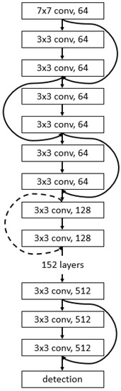
Figure 1.
Architecture diagram of the ResNet-152 convolutional neural network (CNN) used.
Both convolutional neural networks were implemented using the Python programming language [22] supported by the TensorFlow [23] library. A manual training set annotation was performed with the help of the VGG Image Annotator Tool (VIA) [24].
For the deep-learning purposes, a dataset containing 220 3D body scans with the known locations of the body’s landmarks was used −200 for training (148 male and 52 female) and 20 (10 male and 10 female) for validation and testing. Volunteers’ age ranged from 22 to 55 years old, weight from 55 to 105 kg, and height from 150 to 205 cm. In order to ensure satisfying results despite using datasets of significantly limited quantity, transfer learning [25] was applied using the Microsoft COCO dataset [26]. The transferred knowledge pertained to the capability of object segmentation from the background and shape recognition. This method utilized precalculated weights for learning time reduction and accuracy enhancement. All participants were asked to take standing poses with arms and legs spread [27]. Scans were captured using the multi-directional structured light method [28]. The data were acquired in the form of a 3D point cloud in Euclidian space. A marked sample scan is shown in Figure 2.
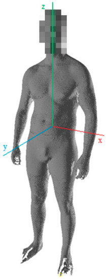
Figure 2.
Sample of input with marked axis, where x—width, y—depth and z—height.
Implemented neural networks were trained to detect and classify 22 standardized landmarks [29,30,31]. Abbreviations, names and norm references of utilized characteristic points are presented in Table 1.

Table 1.
List of selected standardized human body landmarks, where L—left and R—right.
3. Methods
Machine-learning data preparation for the body landmarking is not a straightforward process. The proposed mid-surface approach was compared to and designed on top of the current state-of-the-art method by Xi et al. [17] utilizing orthogonal projection. No code was attached to the original article, so we directly followed the processing steps described and implemented them as precisely as possible. It has to be noted, however, that the preprocessing step was extended by surface smoothing to achieve comparable results. The original approach was divided into five parts: initial processing, specific layer calculation, projection, image generation, and automatic marking process. Between the fourth and fifth steps, the machine-learning task was performed with the use of the generated images. The workflow with a step-by-step visualization is presented in Figure 3.
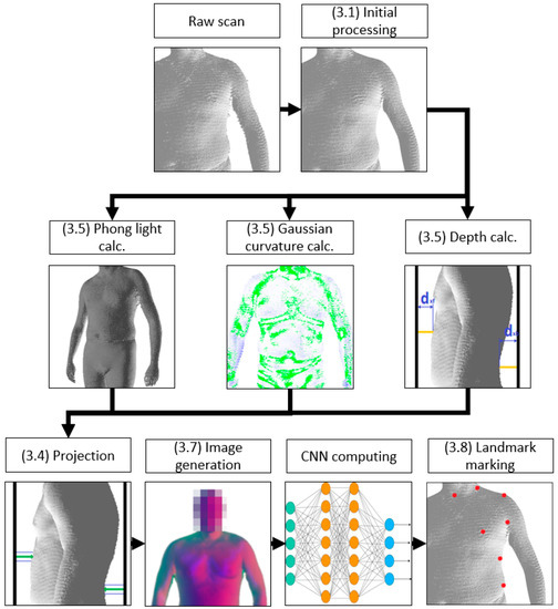
Figure 3.
Workflow of orthogonal projection method.
In contrast, the mid-surface method was divided into eight separate subprocesses, which are described in detail in the following paragraphs. The workflow is presented in Figure 4.
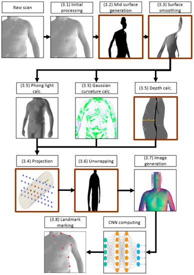
Figure 4.
Workflow of mid-surface projection method. Bold brown frames represent steps, which differed from our approach compared to the orthogonal projection approach.
For both methods, the same 3D human whole body point clouds were used as an input. They were also outputting similar data—3D scans overlaid with the detected and marked landmarks.
3.1. Initial Processing
Raw clouds of points were noisy and needed to be smoothed. Despite the possible loss of some fine surface geometry details, the smoothing process could not be avoided and overall benefits exceeded potential losses. This step was essential due to its significant impact for normal vector generation. Such unwanted noise could adversely alter all of the later specific layer calculations. It was also performed in the same way for both of the methods, so it did not affect their comparison. Therefore, we decided to perform at least a simple 3D plane smoothing. For every point, a best-fit 3D plane was generated by using k-nearest neighbors points. When the plane was generated, actual points were projected onto it [32]. A comparison between raw and smoothed scans is provided in Figure 5.
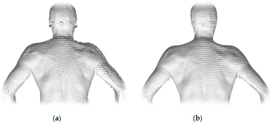
Figure 5.
Comparison of raw (a) and smoothed (b) scans.
The mid-surface scans were additionally segmented using slicing and contour analysis [14]. The body was divided into a head, arms, upper torso, lower torso, hips and legs, as shown in Figure 6.
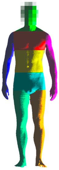
Figure 6.
Three-dimensional (3D) body segmented scan colored according to the body parts (head, arms, upper/lower torso, hips, and legs.
3.2. Mid-Surface Projection
Generation of the mid-surface projection was a fundamental part of the proposed method. In order to calculate it, the scans were divided into 2 mm thick horizontal slices separately for different segments. A mid-surface plane was defined as perpendicular to the transverse plane (XY). It was further aligned to the best-fit line of the flattened slice surface points using the Root Mean Square algorithm. Utilized formulas for slope (1) and offset (2) calculations are presented below:
where a is the slope; b is the offset; n is the quantity of points in the slice; i is the number of currently considered points in the slice; and xi, yi, zi are the coordinates of the ith point in slice.
The algorithm depended on the proportion of the slice and could output one of the two possible slope coefficients, as shown in Figure 7. For unification, if the angle α between sagittal plane (YZ, marked in yellow) and the calculated mid-surface best-fit alignment line was less than 45° or greater than 135°, the surface was rotated by 90°. When the plane was consistently oriented, segment points were projected perpendicularly onto it. After performing the process for each slice separately, the mid-surface projection was obtained.
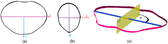
Figure 7.
Two possible calculated surfaces, not requiring rotation (a) with corresponding 3D view (c), and requiring rotation (b). Best-fit line is represented by purple solid lines in (a,b) and blue line in (c). Reoriented dotted line is shown in (b). Calculation of angle α based on sagittal plane (YZ, yellow) and best-fit line (blue) from slice points (purple) is presented in (c).
3.3. Mid-Surface Smoothing
Typically, the generated surface was prone to imperfections. They were mostly caused by scan defects or inaccurate plane estimation due to the insufficient number of points in the provided slice. To reduce its negative influence on the further processing, the mid-surface was smoothed by averaging slopes and offset from the nearest neighborhood planes (20 planes per side, in the range of 80 mm). This process was executed for each segment separately, with the exception of boundaries, where values from the adjoined body parts were included (e.g., torso and legs). As a result, the surface became continuous and smooth, as can be seen in Figure 8.
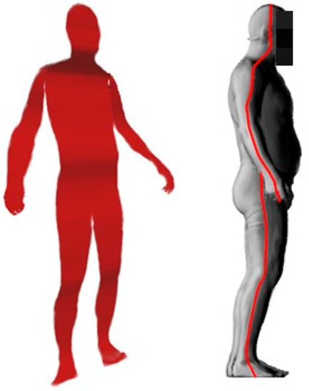
Figure 8.
Generated mid-surface projection after smoothing process.
3.4. Phantom Projection
In case of the reference Xi et al. orthogonal approach, a projection cloud consisting of homogenously distributed points was generated in form of the 2 mm raster. For each point, a cuboid treated as a casting ray was utilized to retrieve the input scan’s surface geometric information. Specific points with the shortest distance from the bounding box face as well as its nearest neighborhood inside the cuboid were considered. Assigned layer values and coordinates from the selected scan’s area were averaged and saved to a raster point.
In the proposed method, the calculation of normal vectors for the mid-surface had to be calculated. When preprocessing was done, the projection could begin. For each point of a mid-surface, a cylindrical search (where the central axis was aligned with the normal vector traced from the point) with diameter of 2 mm was performed. Points from the scan which were inside the cylinder were averaged (x, y, z coordinates, previously calculated layer values (see calculation of layers step 3.5), and body part correspondence). Such data were used to create new phantom points. Their positions and layer values were directly projected to the surface points. This procedure was performed twice, separately for points in front of and behind the body surface. The visualization of the process is shown in Figure 9.
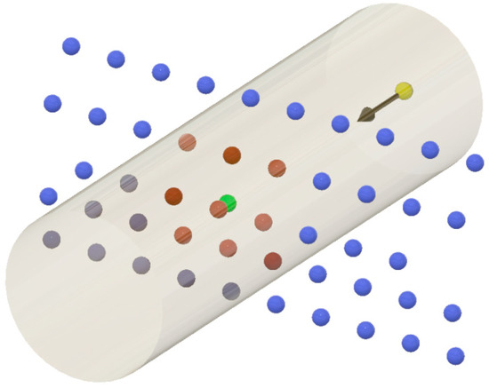
Figure 9.
Cylinder traced from one of the mid-surface points (yellow), along its normal vector (black) and the body surface points (blue). The output phantom point (green) was calculated as a center of mass using the range of the scan points (brown) inside the cylinder.
3.5. Calculation of Layers
Three layers—depth, Gaussian curvature, and light [17]—were required to obtain body landmarks automatically. Prior to the specific layer computation, normal vectors of the cloud point had to be computed in order to obtain repeatable and satisfying results. After the initial preprocessing stage, light and Gaussian curvature [33] computations were performed. Light intensity was calculated using the Phong model [34], assuming an upfront light source. Afterwards, the depth for the orthogonal projection method was calculated as a distance from a point in a bounding box face (front and back separately) to the nearest point on the orthogonally casted ray’s path (see projection step), as shown in Figure 10.
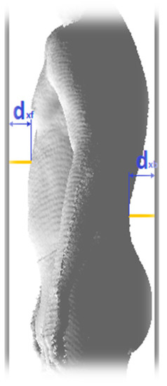
Figure 10.
Scan with marked front and back face of bounding box and corresponding exemplary depth measurements.
The color-mapped layers for the orthogonal projection method are shown in Figure 11.
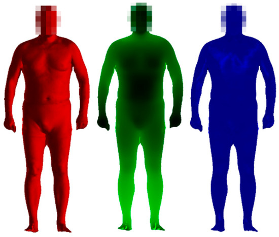
Figure 11.
A visualization of calculated layers values for the orthogonal projection: light intensity (red), depth (green) and curvature (blue).
Both methods shared the same curvature and light layers. However, depth in the proposed method was calculated differently, as the distance between the position of the actual point from the mid-surface and the certain phantom point (see projection step). A layer representation is provided in Figure 12.
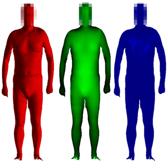
Figure 12.
A visualization of calculated layers values for the mid-surface projection: light intensity (red), depth (green) and curvature (blue).
3.6. Unwrapping
The aim of the unwrapping step is a preparation of the mid-surface for the future image generation. At this point, the impact of the pose imperfections was reduced due to the nature of unwrapping unification. The process was divided into two parts: flattening and extending. The flattening step was responsible for the proper handling of the twisted scans (e.g., with the misaligned middle planes of the head and the torso). In this step, for each plane, the middle point (Pm) was calculated and treated as a pivot for a rotation of the surface points. As a result of that process, all faces became parallel to the coronal plane (XZ). A visualization of the process is shown in Figure 13.
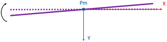
Figure 13.
Visualization of flattening process.
The next step was extending the mid-surface. This process aimed to transfer a 3D surface into a 2D surface and reduce the negative impact of a limb’s inclination. The offset of the plane (along the y-axis) was recalculated with the following formula:
where n is the number of currently processed slices; hn is the average height coordinate (along z-axis) of points from the considered slice, where the point of interest belonged to a flat surface; hn−1 is the average height of the previous slice; yn is the depth coordinate of the considered line from the mid-surface; yn−1 is the depth coordinate of the previous line from the mid-surface; zn and zn−1 are the height coordinates; ∆z is the difference in height between the point of interest and the average z for the selected slice. The height of the first slice was assumed as the y coordinate. Calculations were carried out separately for all segments, except for the borders. A scheme of the extraction is shown in Figure 14.
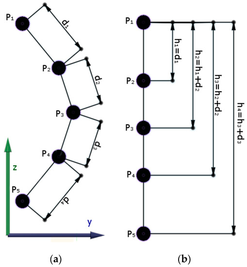
Figure 14.
Scheme of mid-surface before (a) and after (b) extension process. Black dots represent averaged y and z coordinates of slice (P1–P5), with marked distances between them (d1–d4).
3.7. Image Generation
The final operation, which needed to be performed before CNN detection and training, was the generation of an image from a 2D surface (mid-surface in the case of the presented method and boundary face for the original approach). This was done by the direct projection of points into pixels, which took the following values: intensity of light from the Phong model, R (red); Gaussian curvature, G (green); depth, B (blue). All values were normalized in a range from 0 to 1. To improve separation between the front and back, two different backgrounds were used (white and black, respectively). Due to noise, which could occur on the generated image, median filtering was performed as post-processing. An output in the form of an image was provided to the convolutional neural networks for the detection and classification task. Examples of the generated images are shown in Figure 15.
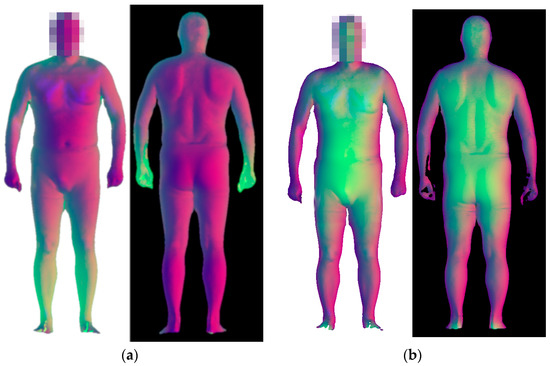
Figure 15.
Images generated using orthogonal projection (a) and mid-surface projection (b).
3.8. Automatic Marking Process
The results of CNN computation were positions of pixels in the image linked to the class names of recognized landmarks. To transfer this 2D data into 3D-point coordinates, an automatic marking process was required. To preserve the proportions, the pixel position from the image was used to create the phantom point in an unwrapped mid surface. To select the specific spot in the scan, the point from the mid surface with the shortest distance from the phantom point was chosen. Each point of the mid surface contained previously collected information (Section 3.4) regarding the coordinates of the represented spot on the scan. Having the expected position, the specific point from the scan could be selected.
4. Results
To evaluate the accuracy of the two presented methods, a comparison on 20 volunteers (10 female, 10 male) of various postures was conducted. To check if the proposed method is defect-resistant, in the validation group, there were two scans with significant flaws in the form of holes and five with lesser defects; these are presented in Figure 16. Each scan was processed using both methods.
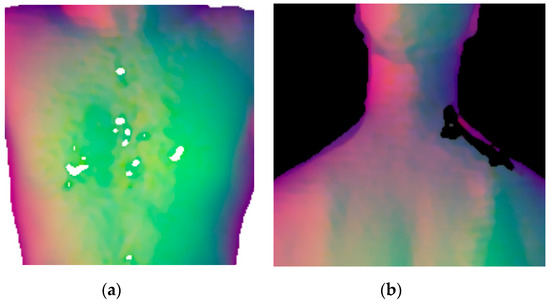
Figure 16.
Examples of data with different types of defects: lesser (a) and significant (b).
The machine-learning task was performed on the same neural networks with the use of identical configurations and similar training duration expressed in the number of epochs (about 55,000). To compare results, distances between computed and manually-marked landmarks (considered as ground truth points) were measured. Distances were calculated using the following formula (4):
where d is distance; xc, yc, zc are computed coordinates of the landmark; and xm, ym, zm are coordinates of the manually-marked characteristic point. Symmetrical characteristic points were considered as the same landmark. For all types, arithmetic means and standard deviations were calculated. Results are presented in Figure 17 and provided in Table 2.
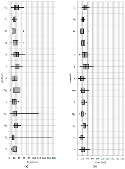
Figure 17.
Box chart of error distribution for orthogonal (a) and mid-surface projection (b).
Table 2.
Experimental results expressed in mm. Scores of the orthogonal projection were divided into the raw distances and filtered gross error values (presented in parentheses if applicable).
5. Discussion
Although the manual method is not perfect, it was chosen as a ground truth reference, due to no commercial system being available.
The results provided by both methods varied for different types of landmarks. For the mid-surface projection, the highest average values of errors were noted for the lowest rib point (37.5 mm), crotch CR (29.2 mm), and highest hip points HL, HR (29.1 mm). All those points are related to lower parts of the torso, for which the shape was strongly affected by the weight of volunteers. The best performance was achieved for neck back neck point NB (13.9 mm) and lowest chin point RL, RR (15.1 mm), which were significantly less dependent on the body silhouette.
Similar dependency on variation could have been observed for the orthogonal projection method, where the distribution of average distances and standard deviation showed that the best results were gained for chin lowest CL (16.1 mm) and wrist points WL, WR (18.9 mm). The worst performance after filtering was noted for the elbow EL, ER (32.7 mm) landmarks.
Based on a comparison of the distribution of averages for different landmarks, an improvement for head- and limb-related ones could have been observed with the use of the mid-surface projection. It was caused by two factors. Firstly, in the case of the mid-surface approach, limbs were straightened during the unwrapping process, which led to reduction of the inclination impact and as a result decrease imperfect pose influence. Secondly, extrusion resulted in a reduced error per pixel. That effect can be observed on the neck back point (33% decrease of the distance in the case of the mid-surface projection).
On the other hand, the orthogonal projection proved better performance for landmarks from the lower part of the torso. This was related to the convexity influence on the resolution of the projection. With rapid curvature changes, such as for the stomach area, rays of the mid-surface projection spread radially. The related points were more spatially separated than in the case of the orthogonal projection, which resulted in an overall lower resolution for this region. The possible solution of this problem would be the application of various resolutions by interpolation in the mid-surface projection in the region of the lower torso. This would lead to an increased density of rays and resolution. An alternative approach would be the utilization of a hybrid method consisting of the mid-surface and the orthogonal projections dependent on body part.
Analysis of the process and results obtained showed the difference in standard deviation between both methods. In the case of the orthogonal projection, defects in the form of holes in the scan can occur when the wrong face of the model is visible. The NB, AFF and CL landmarks were characterized by a significant increase of an error (up to 172.8 mm) for the incomplete data. This led to a strong decrease in the accuracy of the automatic marking process. Using the mid-surface method, such effects were minimized due to the projection from within the scan, where only one face was taken into consideration at once. In conclusion, a resistance to incomplete input data was improved. A comparison of images obtained via the mid-surface and the orthogonal back projections is presented in Figure 18. In the orthogonal approach, the unwanted front face of the scan can be seen and is mixed with the projected back view.
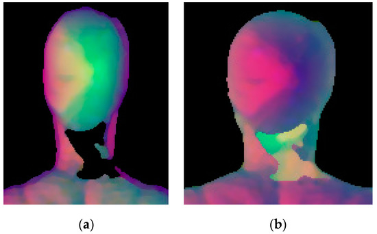
Figure 18.
Comparison of images generated via mid-surface (a) and orthogonal projection (b) for back view.
6. Conclusions
In this paper, we propose a new method of data preparation for the detection of landmarks on 3D body scans with the use of mid-surface projection. We presented the process workflow and provided a detailed description of the algorithms used.
Experimental results showed that the mid-surface projection performed better than the orthogonal projection, achieving on average 14% lower error. The presented method’s performance varied depending on the location of the body part. Better scores were noted for the head, neck, and limbs, but the method was less effective for points located on the lower torso.
The authors confirmed that the mid-surface projection was substantially less affected by scan imperfections in the form of holes, which caused significant errors in the orthogonal approach. Furthermore, the negative influence of the limb inclination was reduced with the use of the unwrapping process of the demonstrated method.
For improvement of general accuracy (especially in case of the landmarks situated in the lower part of torso), an extensive database needs to be established (characterized by multiple scans of various poses, silhouettes and ages). It would be beneficial for CNN training, detection and classification.
Author Contributions
M.K. contributed to conceptualization and the writing of the manuscript; Ł.M. revised the manuscript, providing insightful suggestions and English corrections; R.S. provided suggestions, supervision and organization of the manuscript; All authors have read and agreed to the published version of the manuscript.
Funding
This research received no external funding.
Conflicts of Interest
The authors declare no conflict of interest.
References
- Bendels, G.H.; Klein, R.; Samimi, M.; Schmitz, A. Statistical shape analysis for computer aided spine deformity detection. J. WSCG 2005, 13, 57–64. [Google Scholar]
- Michoński, J.; Witkowski, M.; Sitnik, R.; Glinkowski, W.M. Automatic recognition of surface landmarks of anatomical structures of back and posture. J. Biomed. Opt. 2012, 17, 056015. [Google Scholar] [CrossRef] [PubMed]
- Chu, C.; Belavý, D.L.; Armbrecht, G.; Bansmann, M.; Felsenberg, D.; Zheng, G. Fully Automatic Localization and Segmentation of 3D Vertebral Bodies from CT/MR Images via a Learning Based Method. PLoS ONE 2015, 10, e0143327. [Google Scholar] [CrossRef] [PubMed]
- Vezzetti, E.; Calignano, F.; Moos, S. Computer-aided morphological analysis for maxilla-facial diagnostic: A preliminary study. J. Plast. Reconstr. Aesthetic Surg. 2010, 63, 218–226. [Google Scholar] [CrossRef]
- Dutreve, L.; Meyer, A.; Orvalho, V.; Bouakaz, S. Easy Rigging of Face by Automatic Registration and Transfer of Skinning Parameters. In Computer Vision and Graphics. Lecture Notes in Computer Science; Bolc, L., Tadeusiewicz, R., Chmielewski, L.J., Wojciechowski, K., Eds.; Springer: Berlin/Heidelberg, Germany, 2010; Volume 6374. [Google Scholar] [CrossRef]
- Dagnes, N.; Marcolin, F.; Vezzetti, E.; Sarhan, F.R.; Dakpé, S.; Marin, F.; Mansour, K.B. Optimal marker set assessment for motion capure of 3D mimic facial movements. J. Biomech. 2019, 93, 86–93. [Google Scholar] [CrossRef]
- Duan, L.; Yueqi, Z.; Ge, W.; Pengpeng, H. Automatic three-dimensional-scanned garment fitting based on virtual tailoring and geometric sewing. J. Eng. Fibers Fabr. 2018, 14, 1–16. [Google Scholar] [CrossRef]
- Lacko, D.; Huysmans, T.; Vleugels, J.; De Bruyne, G.; Van Hulle, M.; Sijbers, J.; Verwulgen, S. Product sizing with 3D anthropometry and k-medoids clustering. Comput. Aided Des. 2017, 91, 60–74. [Google Scholar] [CrossRef]
- Steimle, S.; Bergstrom-Lehtovirta, J.; Weigel, M.; Nittala, A.S.; Boring, S.; Olwal, A.; Hornbæk, K. On-Skin Interaction Using Body Landmarks. IEEE Comput. 2017, 50, 19–27. [Google Scholar] [CrossRef]
- Kouchi, M.; Mochimaru, M. Errors in landmarking and the evaluation of the accuracy of traditional and 3D anthropometry. Appl. Ergon. 2011, 42, 518–527. [Google Scholar] [CrossRef]
- Lu, J.; Wang, M. Automated anthropometric data collection using 3D whole body scanners. Expert Syst. Appl. 2008, 35, 407–414. [Google Scholar] [CrossRef]
- Ferrario, V.F.; Sforza, C. Anatomy of emotion: A 3D study of facial mimicry. Eur. J. Histochem. 2007, 51, 45–52. [Google Scholar]
- Galantucci, L.M.; Di Gioia, E.; Lavecchia, F.; Percoco, G. Is principal component analysis an effective tool to predict face attractiveness? A contribution based on real 3D faces of highly selected attractive women, scanned with stereophotogrammetry. Med. Biol. Eng. Comput. 2014, 52, 475–489. [Google Scholar] [CrossRef] [PubMed]
- Markiewicz, Ł.; Witkowski, M.; Sitnik, R.; Mielicka, E. 3D anthropometric algorithms for the estimation of measurements required for specialized garment design. Expert Syst. Appl. 2017, 85, 366–385. [Google Scholar] [CrossRef]
- Vezzetti, E.; Marcolin, F. 3D Landmarking in Multiexpression Face Analysis: A Preliminary Study on Eyebrows and Mouth. J. Aesthetic Plast. Surg. 2014, 38, 796–811. [Google Scholar] [CrossRef] [PubMed]
- Boscaini, D.; Masci, J.; Melzi, S.; Bronstein, M.M.; Castellani, U.; Vandergheynst, P. Learning class-specific descriptors for deformable shapes using localized spectral convolutional networks. Comput. Graph. Forum 2015, 34, 13–23. [Google Scholar] [CrossRef]
- Xi, P.; Shu, C.; Goubran, R. Localizing 3-D Anatomical Landmarks Using Deep Convolutional Neural Networks. In 2017 14th Conference on Computer and Robot Vision (CRV); IEEE: Piscataway, NJ, USA, 2017; pp. 1–6. [Google Scholar] [CrossRef]
- Simonyan, K.; Zisserman, A. Very deep convolutional networks for large-scale image recognition. arXiv 2014, arXiv:1409.1556. [Google Scholar]
- Russakovsky, O.; Deng, J.; Su, H.; Krause, J.; Satheesh, S.; Ma, S.; Huang, Z.; Karpathy, A.; Khosla, A.; Bernstein, M.; et al. ImageNet Large Scale Visual Recognition Challenge. Int. J. Comput. Vis. 2015, 115, 211–252. [Google Scholar] [CrossRef]
- Redmon, J.; Farhadi, A. Yolov3: An incremental improvement. arXiv 2018, arXiv:1804.02767. [Google Scholar]
- He, K.; Zhang, X.; Ren, S.; Sun, J. Deep Residual Learning for Image Recognition. In Proceedings of the IEEE Conference on Computer Vision and Pattern Recognition), Las Vegas, NV, USA, 27–30 June 2016; IEEE: Piscataway, NJ, USA, 2016; pp. 770–778. [Google Scholar]
- Oliphant, T.E. Python for Scientific Computing. Comput. Sci. Eng. 2007, 9, 10–20. [Google Scholar] [CrossRef]
- Schrimpf, M. Should I use TensorFlow. arXiv 2016, arXiv:1611.08903. [Google Scholar]
- Dutta, A.; Zisserman, A. The VIA Annotation Software for Images, Audio and Video. In Proceedings of the 27th ACM International Conference on Multimedia, Nice, France, 21–25 October 2019. [Google Scholar]
- Yosinski, J.; Clune, J.; Bengio, Y.; Lipson, H. How transferable are features in deep neural networks? In Advances in Neural Information Processing Systems; Ghahramani, Z., Welling, M., Cortes, C., Lawrence, N.D., Weinberger, K.Q., Eds.; Annual Conference on Neural Information Processing Systems: Montreal, QC, Canada, 2014; Volume 27, pp. 3320–3328. [Google Scholar]
- Lin, T.; Maire, M.; Belongie, S.; Hays, J.; Perona, P.; Ramanan, D.; Dollár, P.; Zitnick, C.L. Microsoft COCO: Common Objects in Context. In Computer Vision—ECCV 2014. Lecture Notes in Computer Science; Springer: Cham, Switzerland, 2014. [Google Scholar] [CrossRef]
- ISO 20685-1:2018. Available online: https://www.iso.org (accessed on 12 December 2019).
- Sitnik, R.; Kujawińska, M.; Woźnicki, J. Digital fringe projection system for large-volume 360-deg shape measurements. Opt. Eng. 2002, 41, 443–449. [Google Scholar] [CrossRef]
- McDonald, C.; Concept, G.; Wu, Y.; Ballester, A.; Stahl, M. IEEE Industry Connections (IEEE-IC) Landmarks and Measurement Standards Comparison in 3D Body-model Processing. In Proceedings of the IEEE White Paper; IEEE: Piscataway, NJ, USA, 22 February 2018. [Google Scholar]
- ISO 7250-1:2017. Available online: https://www.iso.org (accessed on 12 December 2019).
- ISO 8559-1:2017. Available online: https://www.iso.org (accessed on 12 December 2019).
- Muralikrishnan, B.; Raja, J. Least-squares best-fit lane and plane. In Computational Surface and Roundness Metrology; Springer: London, UK, 2009; pp. 121–130. [Google Scholar] [CrossRef]
- Gamriella, R.; Swartz, B. Curvature Estimation for Unstructured Triangulations of Surfaces; Technical Report; LA-UR-03-8240; Los Alamos National Laboratory: Los Alamos, NM, USA, 2003. [Google Scholar]
- Strauss, P.S. A realistic lighting model for computer animators. IEEE Comput. Graph. Appl. 1990, 10, 56–64. [Google Scholar] [CrossRef]


© 2020 by the authors. Licensee MDPI, Basel, Switzerland. This article is an open access article distributed under the terms and conditions of the Creative Commons Attribution (CC BY) license (http://creativecommons.org/licenses/by/4.0/).