Research on a Noise Reduction Method Based on Multi-Resolution Singular Value Decomposition

Abstract

Reducing noise pollution in signals is of great significance in the field of signal detection. In order to reduce the noise in the signal and improve the signal-to-noise ratio (SNR), this paper takes the singular value decomposition theory as the starting point, and constructs various singular value decomposition denoising models with multiple multi-division structures based on the two-division recursion singular value decomposition, and conducts a noise reduction analysis on two experimental signals containing noise of different power. Finally, the SNR and mean square error (MSE) are used as indicators to evaluate the noise reduction effect, it is verified that the two-division recursion singular value decomposition is the optimal noise reduction model. This noise reduction model is then applied to the diagnosis of faulty bearings. By this method, the fault signal is decomposed to reduce noise and the detail signal with maximum kurtosis is extracted for envelope spectrum analysis. Comparison of several traditional signal processing methods such as empirical modal decomposition (EMD), ensemble empirical mode decomposition (EEMD), variational mode decomposition (VMD), wavelet decomposition, etc. The results show that multi-resolution singular value decomposition (MRSVD) has better noise reduction effect and can effectively diagnose faulty bearings. This method is promising and has a good application prospect.

1. Introduction

Signals are inevitably subject to natural and man-made interference during acquisition and transmission. In high precision data analysis, even extremely weak noise interference can have a huge impact on the analysis results. Therefore, before signal processing it is necessary to first denoise it. Whether the noise can be removed from the disturbed observation signal is related not only to the nature of the interference and the form of the signal, but also to the manner in which the signal is processed. In practical applications, finding the best processing method to reduce noise aiming at different types of signal and interference has been a widely discussed problem in the field of signal processing.

In recent decades, many signal denoising methods have been proposed, such as the empirical mode decomposition proposed by Huang [1], the ensemble empirical mode decomposition, and the variational mode decomposition (VMD), etc. Among them, EMD has obvious advantages in dealing with non-stationary and nonlinear data. It is suitable for analyzing nonlinear and non-stationary signal sequences and has good SNR. The key of this method is empirical mode decomposition, which can decompose complex signal into a finite number of intrinsic mode functions (IMFs) [2,3]. The decomposed IMF components contain local characteristic signal with different time scales of the original signal. However, EMD has non-negligible end-point effects and modal aliasing; EEMD [4] is a noise-assisted data analysis method proposed aiming at the deficiency of EMD. While using the noise-assisted signal to add the white noise background signal with a uniformly distribute, the signal regions with different scales will be automatically mapped to the appropriate scale related to the background white noise, which reduces the influence of the modal aliasing phenomenon, but the method has a large amount of computation, and the modal component is not controlled, it is easy to cause the function to not converge, which affects the accuracy of the algorithm [5]; VMD is to realize complex signal decomposition by finding the optimal solution of constrained variational model. Its essence is adaptive Wiener filtering [6], but the K value selection of variational mode decomposition will affect the decomposition result. In [7], a feature extraction method based on VMD and Hilbert transform is proposed. According to the power spectrum of PD signal, the double-threshold screening method is used to determine the number of decomposition modes in the VMD algorithm. Although the above several methods can realize the processing of noise signals, they all have the inevitable defects of modal aliasing.

Singular value decomposition (SVD) is an orthogonal transformation that could transform the original matrix into a diagonal matrix whose eigenvalues reflect some of the main features of the original matrix. As a data processing method, SVD has been successfully applied to signal denoising processing and proved to be effective in avoiding modal aliasing. The main application of singular value decomposition in statistics is the principal component analysis (PCA), which can be used in pattern recognition [8,9,10,11], data dimensionality reduction [12,13], filter design [14,15], denoising [16,17], feature extraction and weak signal separation [18,19,20,21,22], face recognition [23,24] and many other fields, and it has gained important applications. In10, the application of SVD in pattern recognition of partial discharge signals is studied. The singular value power percentage is defined as the eigenvector of the partial discharge signal, and it is verified that the discharge signal eigenvalue vector constructed with the singular value power percentage can reflect the original signal characteristics; In [17], the order of the effective rank is determined by the fast Fourier transform of the noise signal, and the reconstruction matrix is determined for SVD decomposition to reduce the noise of the Gaussian white noise-contaminated signal, the output SNR is improved. In [21], at the basis of SVD, the singular value decomposition based on slip matrix sequence is proposed, and the difference spectrum, main singular sum, maximum eigenvalue reconstruction and optimal filter design are introduced to realize the fault feature extraction of rolling bearings under noise background. The above results obtained by the SVD method for noise reduction are essentially the same level of spatial and identical resolution results, and cannot reveal the signal profile and detail features at different levels. Drawing on the idea of wavelet multi-resolution analysis, Zhao [25] proposed a new research idea, using the recursive idea to construct the signal into a second-order matrix, and perform singular value decomposition on the matrix layer by layer to obtain the decomposition results of signals in different levels of space and different resolutions, so as to achieve multi-resolution decomposition similar to wavelet analysis that can decompose signals into a series of different hierarchical subspaces. This is essentially different from previous SVD-based signal processing methods, called MRSVD. Huang [26] proposed a method based on generalized morphological filtering and multi-resolution singular value decomposition. The signal is denoised by MRSVD and the kurtosis criterion is used to select the most detailed fault signal for Hilbert envelope spectrum analyze to obtain the characteristic information of the fault signal. Malini [27] decomposed the noise image into four different frequency bands by multi-resolution singular value decomposition, reconstructs the separated high-frequency detailed sub-bands to obtain the noise image, and selects the appropriate threshold to remove the noise signal. The signal noise reduction mentioned in the above several documents does not involve the analysis of the noise reduction effect, and does not consider the factors affecting the noise reduction effect.

Based on the theory of MRSVD, this paper studies the noise reduction model of multi-division structure MRSVD and summarizes it. The SNR and MSE are used as evaluation indexes to verify the several noise reduction models, and the MRSVD is obtained under different conditions and then comparing MRSVD with traditional noise reduction methods, the results show that the MRSVD method avoids defects such as EMD and EEMD to a certain extent, and also has better adaptability and robustness. The results show that the MRSVD method avoids EMD to a certain extent. Defects such as EEMD have the advantages of better adaptability and robustness, and have certain research value in the application of noise reduction. Specifically, the organizational structure of this paper is as follows: Section 2 briefly introduces the methods, including MRSVD and multi-division structure MRSVD, and introduces the noise reduction model and evaluation indicators; Section 3 conducts simulation analysis and case verification, and analyzes and discusses the results. The conclusions are given in Section 4.

2. Method Overview

2.1. MRSVD

2.1.1. The Two-Division Recursion SVD

The two-division recursion SVD is based on the singular value decomposition, adding the idea of the two-division25, and reconstructing the signal into a Hankel matrix with two rows, realizing a decomposition of complex signals into sub-spaces of different levels, it is also called MRSVD.

For an one-dimensional signal $X=\{{{\displaystyle x}}_1,{{\displaystyle x}}_2\begin{array}{cc}\dots & \end{array}{{\displaystyle x}}_N\}$, a Hankel matrix A is constructed by using the two-division recursion SVD method as shown in Equation (1):

$$A=\left[\begin{array}{l}{{\displaystyle x}}_1,{{\displaystyle x}}_2,\begin{array}{cc}\cdot \cdot \cdot & {{\displaystyle x}}_{N-1}\end{array}\\ {{\displaystyle x}}_2,{{\displaystyle x}}_3,\begin{array}{cc}\cdot \cdot \cdot & {{\displaystyle x}}_N\end{array}\end{array}\right]$$

(1)

Then, the singular value decomposition of the matrix A is performed to obtain Equation (2):

$$A={\sigma }_{11}{u}_{11}{v}_{11}^T+{\sigma }_{12}{u}_{12}{v}_{12}^T$$

(2)

where ${\sigma }_{11}$ and ${\sigma }_{12}$ are the two singular values obtained by the first decomposition and ${\sigma }_{11}$ > ${\sigma }_{12}$,$u_{11}$ and $u_{12}$ are the vectors formed by the first two rows of the first decomposition of the matrix U. $v_{11}$ and $v_{12}$ are the vectors formed by the first two rows of the matrix V. The decomposition diagram is shown in Figure 1. Align symbols correctly.

${\sigma }_{11}$ is the larger singular value, the corresponding reconstructed sub-signal $A_1$ is the approximate signal obtained by the first decomposition; the smaller singular value ${\sigma }_{12}$ corresponds to the reconstructed sub-signal $D_1$, which is the detailed signal obtained by the first decomposition. The approximate signal $A_1$ is selected to continue to construct the Hankel matrix with the number of rows 2 for the SVD decomposition of the next layer, and the original signal is decomposed successively into a set of detail signals and approximation signals with different resolutions.

Reconstructing matrix $A_0$ using Equation (3):

$$A_0=A_M+{\displaystyle \sum _{j=1}^M{D}_j}$$

(3)

It can be seen from the above decomposition process that the signal reconstruction requires only a simple summation of $D_j$ and $A_j$ to obtain the SVD approximation signal $A_{j-1}$ of the upper layer, the original signal $A_0$ can be obtained by analogy, where M is the number of decomposition layers.

2.1.2. Multi-Division Structure MRSVD

MRSVD is constructed by constructing a Hankel matrix with a row number of 2 (described later as the two-division method). Drawing on the idea of it, this paper studies the method of constructing singular value decomposition layer by layer by constructing a Hankel matrix with different structures. The singular value decomposition with different rows of Hankel matrices will form different decomposition methods L, and each decomposition method has different decomposition types N. In this paper, L = 3 and L = 4 (described later as the three-division method and the four-division method) are the main research objects. The component corresponding to the larger singular value in the two-division method is the approximation signal, and the component corresponding to the smaller singular value is the detail signal. The three-division method and the four-division method have three and four singular values respectively, so there are different methods for constructing approximate signals and detailed signals. The decomposition of the three-division method is shown in Figure 2.

There are two types of decomposition in the three-division method (L = 3):

(1) Figure 2a is a Hankel matrix with a row number of three. Each decomposition will result in three signal components. The component corresponding to the first singular value will be regarded as the approximate signal A, and the components corresponding to the last two singular values will be regarded as the detail signal D and d. In this way, D and d is separated as a detail signal during each decomposition, leaving only the approximate signal A for the next layer of decomposition. This type of decomposition is denoted as N = 1.

(2) Figure 2b is another decomposition type of the three-division method. Each decomposition will result in three signal components. The component corresponding to the first two singular values will be regarded as the approximate signal A and a. And the components corresponding to the third singular values will be regarded as the detail signal D. Then the two approximate components A, a are superimposed to construct a Hankel matrix for decomposition of the next layer, and D is separated as a detail component. This type of decomposition is denoted as N = 2.

Similarly, the four-division method (L = 4) has three types of decomposition, N = 1, 2, 3. The specific decomposition and reconstruction process of the three-division and the four-division method is similar to the two-division method. By analogy, the multi-division method is also decomposable, and the p-division method has p-1 types of decomposition.

2.2. Noise Reduction Principle Based on MRSVD

For any discrete digital signal containing noise $y(n)$, it can be expressed as $y(n)=x(n)+\delta (n)$ $n=1,2,\cdot \cdot \cdot N$. Where $x(n)$ is the original signal and $\delta (n)$ is the noise, the specific noise reduction process is as follows:

(1)

The signal containing noise $y(n)$ is constructed to a matrix A that is same as Formula (1).

(2)

Performing the first SVD decomposition on matrix A will obtain two singular values whose reconstructed components can reflect the power concentration of original signal and the noise. Larger singular value will primarily reflect the original signal, while smaller singular value will primarily reflect the noise.

(3)

Zeroing the singular value that reflects the noise, that is to discard the detail signal $D_1={\sigma }_{12}{u}_{12}{v}_{12}^T$, which is equivalent to removing some of the noise in the signal.

(4)

The approximation signal $A_1={\sigma }_{11}{u}_{11}{v}_{11}^T$ is retained to reconstruct the Hankel matrix for decomposition of the next layer, in such a way that decomposition of each layer separates the noise of amplitude $D_i={\sigma }_{i2}{u}_{i2}{v}_{i2}^T$.

Each time the MRSVD is decomposed, in the approximate signal $A_M$, the noise power is reduced by a fraction of the noise power of the previous layer $A_{\mathrm{M}-1}$. This reduced noise is separated into the SVD detail signal, while the original signal has only a small fraction. It is assigned to the SVD detail and its body is basically retained in the SVD approximation signal. When decomposed into a certain number of layers, the noise power in the approximate signal will become very small, and the original signal $x(n)$ is basically retained, thereby achieving the purpose of noise cancellation.

The principle of the three-division method and the four-division method for noise reduction is the same as that of the two-division method. After each layer is decomposed, the components in the detail signal are discarded as noise, and the approximate signal is retained for the next layer of decomposition. The approximate signal and detail signal selection of different decomposition types are as described above.

In order to evaluate the performance of noise reduction, this paper uses two evaluation indicators: SNR and MSE. The following is a brief introduction:

(1) Signal to noise ratio. The SNR is a parameter that describes the ratio of the active component to the noise component in the signal. The larger the SNR, the closer the prediction model is to the ideal model. The SNR mentioned in this paper is calculated by the ratio of signal power to noise power. The specific calculation formula is as shown in Equation (4).

$$SNR=10\times {\log }_{10}\frac{{\displaystyle \sum _{n=1}^N{x}^2(n)}}{{\displaystyle \sum _{n=1}^N{(x(n)-\stackrel{\wedge }{x}(n))}^2}}$$

(4)

where n is the signal sampling point, $x(n)$ is the original signal, $\stackrel{\wedge }{x}(n)$ is the sum of the original signal $x(n)$ and the noise $\delta (n)$, $x^2(n)$ is the power of the original signal, and ${(x(n)-\stackrel{\wedge }{x}(n))}^2$ is the power of the noise signal. It can be seen from Equation (4) that the larger the signal to noise ratio, the larger the power of the original signal and the smaller the noise power.

(2) Mean square error. The MSE is the expected value of the square of the difference between the parameter estimate and the true value of the parameter. The smaller the value of the MSE indicates that the prediction model has better accuracy in describing the experimental data. In this paper, the MSE reflects the magnitude of the noise power. The smaller the value indicates that the less noise in the signal and the better the noise reduction effect. The specific calculation formula is as shown in Equation (5):

$$MSE=\frac{1}{N}{\displaystyle \sum _{n=1}^N{(x(n)-\stackrel{\wedge }{x}(n))}^2}$$

(5)

2.3. Noise Reduction Process

In this paper, the “analysis-optimization-contrast” model is used to study the noise reduction process. The flow chart of this model is shown in Appendix A. It can be seen from this flowchart that the noise reduction model in this paper is mainly divided into four parts. It can be seen from the flow chart that the noise reduction model of this paper is mainly divided into four parts:

Part I: Adding the noise into the signal. Four Gaussian white noises obeying normal distributions with different intensities are added into the experimental signal.

Part II: Building a model. Based on the MRSVD, different noise reduction models are established according to the different values of the decomposition method L and the decomposition type N.

Part III: The selection of the optimal model. Taking the experimental signals adding different noise as the example, the noise reduction analysis on the various models of MRSVD is carried out, and through the comparison between two evaluation indicators, the noise reduction effect of the method is analyzed and discussed under different application scenarios and different parameters, and the optimal model of MRSVD is obtained.

Part IV: Comparison on multiple models. Under the condition of selecting the optimal parameters, the traditional noise reduction model such as EMD, EEMD, VMD, SVD and wavelet decomposition are used to process the simulation signal, which are compared with the MRSVD optimal model obtained in the previous step, and then the conclusion is obtained by an example.

3. Analysis

In this paper, two periodic signals with different frequency components are selected, $x1$ and $x2$, then the white noise $\delta$ with the SNR of −5, 1, 5 and 20 db and obeying the Gaussian distribution N (0, 1) is respectively added in two periodic signals.

Experimental signal 1: $x1=\sin 3t+\sin 20t$, the sampling time is $2\pi$, sampling frequency is 1024 HZ, the number of sampling point is 1024, the frequency of the signal is $f_1=0.4778$ and $f_2=3.183$ respectively.

Experimental signal 2: $x2=\sin (2\pi t)+\sin (20\pi t)+cos(50\pi t)+\sin (100\pi t)$, the sampling time is 1, the sampling frequency is 1000 HZ, the number of sampling point is 1000, the frequency of the signal is $f_1=1$, $f_2=10$, $f_3=25$ and $f_4=50$ respectively. The final simulation signal are Noise1, Noise 2, Noise 3, Noise 4 in Appendix A.

3.1. The Optimal Model of MRSVD

Using different parameters, MRSVD will have different forms, and not all noise reduction models have good effects. Therefore, it is necessary to make a discussion on various models to select the optimal model. In this paper, the different values of the decomposition method L, the decomposition type N and the decomposition layer M are used as variables to draw the relationship curve between two evaluation indicators (SNR, MSE) and the number of decomposition layers in the two-division method, the three-division method, and the four-division under different decomposition types. The optimal model of MRSVD is selected by the specific analysis on the change trend of SNR curve and the MSE curve. 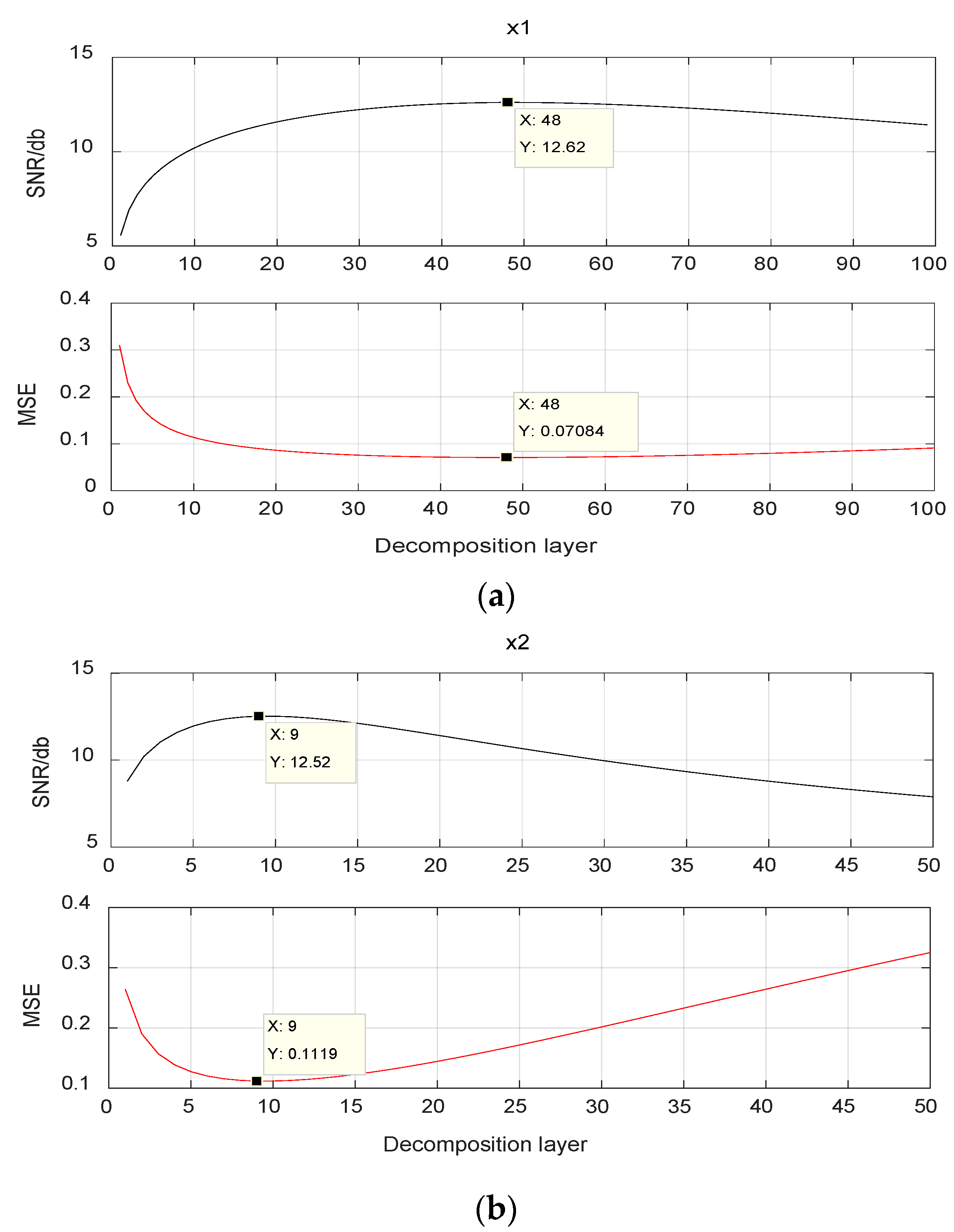Figure 3 is the SNR and MSE curves in the two-division method at an initial SNR of 1 db, where (a) is the curve for $x1$ and (b) is the curve for $x2$.

It can be seen from Figure 3a,b that $x1$ and $x2$ reach the peak SNR at M = 48 and 9, respectively, and the value of MSE just reaches the minimum value. By observing the curve, it can be seen that the initial growth of the SNR curve is faster, then slows down gradually, and begins to decrease after reaching the peak SNR. This is because most of the noise signal is separated into the detail signal at the beginning, and the original signal is basically retained as an approximation signal, so the SNR rises very quickly. When the SNR becomes large, the noise power is already quite small. At this time, the separated noise will inevitably be mixed with some of the original signals, resulting in a decrease in SNR. This is consistent with the principle of noise reduction. An increase on the MSE value indicates that the amplitude of the original signal $x(n)$ is already bigger than the noise-reduced signal $A_M$, and the original signal has been excessively separated into the detail signal. If the decomposition continues, the signal distortion will become more and more serious, and this should be avoided during the noise reduction process. Figure 4 is the SNR and MSE curve in the three-division method at an initial SNR of 1 db, where (a) is the curve for $x1$ and (b) is the curve for $x2$.

It can be seen from Figure 4a,b that the three-division method has two types of decomposition: N = 1 and N = 2. For the three-division method, regardless of the value of decomposition type N of the signal x1 or x2, its SNR reaches the maximum value when M = 1. The SNR curve shows a downward trend and a negative value occurs. If the SNR is negative, then the original signal power is less than the noise power, it shows that the three-division method separates too much of the original signal, which is seen noise wrongly, into the detail signal, that is, the power of the original signal is leaked into the noise, and the signal is severely distorted. It is observed that the value of the MSE increases while the SNR decreases, indicating that the power of the original signal is getting smaller and smaller, which also means that the accuracy of the reconstructed signal after decomposition is gradually degraded as the number of decomposition layers increases.

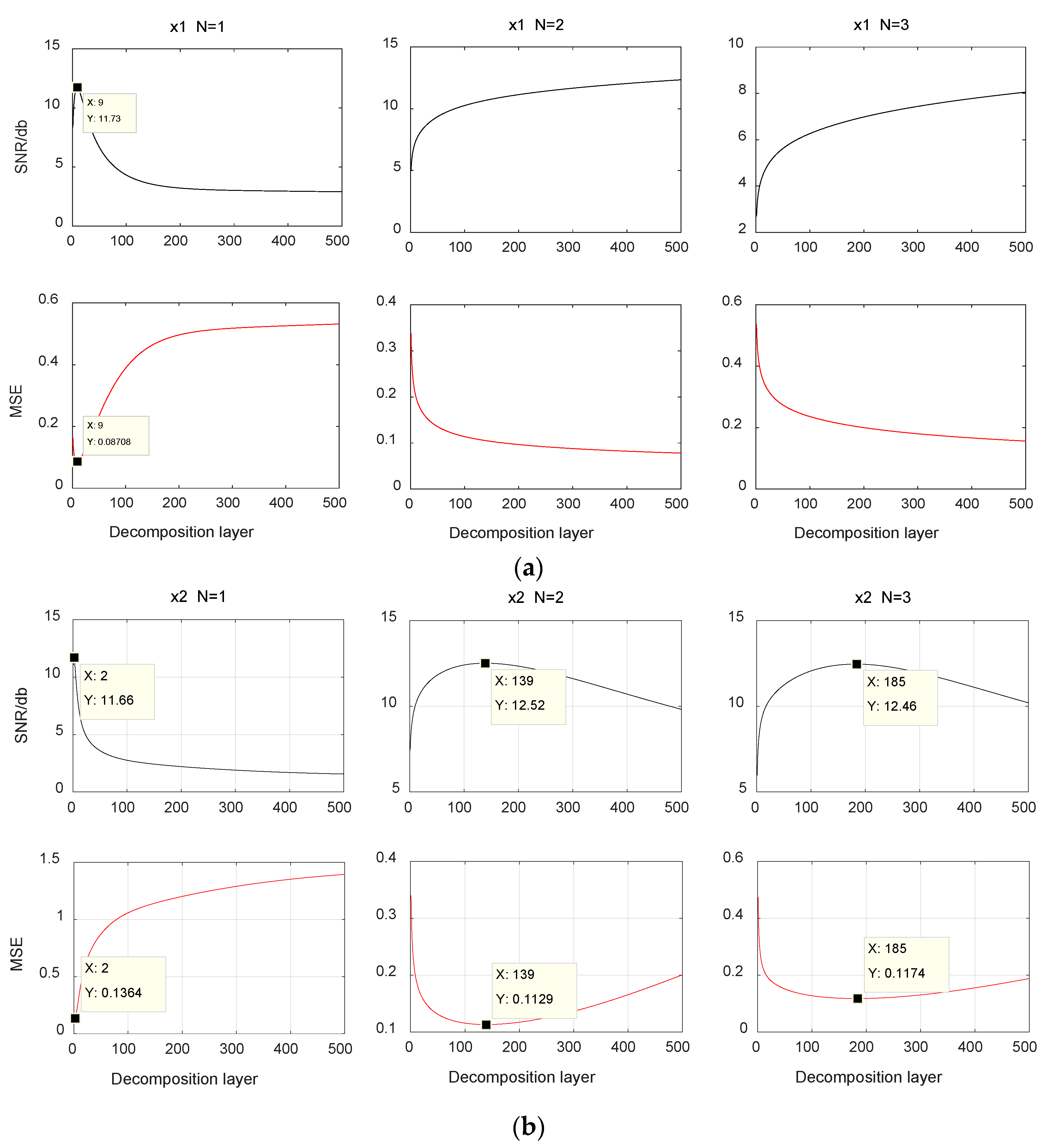
Figure 5 is the SNR and MSE curve in the four-division method at an initial SNR of 1 db, where (a) is the curve for x1 and (b) is the curve for x2. It can be seen from Figure 5a,b that the four-division method has three decomposition types. When N = 1, the SNR of signal x1 increases first and then decreases gradually, and the SNR of x2 has the trend of decreasing, reaching maximum at M = 9 and M = 2 respectively; while N = 2 and N = 3, the SNR has been increasing until M = 500, and the curve becomes very gentle after the number of decomposition layer reach to 500, which indicates that the larger the value of N, the less noise is separated from each layer, and the lower the efficiency of noise reduction. Comparing the peak SNR and minimum MSE of three decomposition types, it can be seen that it has the best decomposition effect when N = 2.

Due to space limitations, the SNR and MSE obtained by adding the white noise with the SNR is respectively −5, 5 and 20 db are given in the tables below.

Table 1. The SNR of different noise reduction models.

SNR/db	$\mathit{x}1$				$\mathit{x}2$
	−5	1	5	20	−5	1	5	20
Two-division	9.182	12.621	14.210	26.718	7.129	12.526	15.618	26.458
Three-division(N = 1)	0.752	6.253	8.071	7.107	2.445	7.375	8.031	6.997
Three-division(N = 2)	−2.186	5.734	7.361	5.585	1.762	7.322	8.039	5.867
Four-division(N = 1)	8.396	11.735	13.374	26.135	7.597	11.662	14.388	22.725
Four-division(N = 2)	5.501	12.611	14.125	30.321	7.012	12. 523	15.606	30.385
Four-division(N = 3)	7.453	8.255	14.212	29.712	6.821	12.463	15.528	29.263

lists the SNR under different noise reduction models,

Table 2. The MSE of different noise reduction models.

MSE	$\mathit{x}1$				$\mathit{x}2$
	−5	1	5	20	−5	1	5	20
Undecomposed	3.141	0.777	0.352	0.009	3.308	0.827	0.286	0.013
Two-division	0.184	0.071	0.022	0.002	0.138	0.112	0.039	0.004
Three-division(N = 1)	0.389	0.247	0.156	0.138	0.399	0.365	0.291	0.244
Three-division(N = 2)	0.552	0.266	0.183	0.118	0.518	0.369	0.272	0.234
Four-division(N = 1)	0.199	0.087	0.033	1.9 × 10−3	0.182	0.129	0.059	0.010
Four-division(N = 2)	0.186	0.073	0.023	6 × 10−4	0.154	0.113	0.039	1.9 × 10−3
Four-division(N = 3)	0.265	0.124	0.036	9.4 × 10−4	0.291	0.117	0.047	2.1 × 10−3

The value of the bold mark indicates the MSE before the decomposition.

shows the MSE values, and

Table 3. The optimal decomposition layers of different noise reduction models.

Decomposition Layer	$\mathit{x}1$				$\mathit{x}2$
	−5	1	5	20	−5	1	5	20
Two-division	78	48	29	7	22	9	8	1
Three-division(N = 1)	1	1	1	1	1	1	1	1
Three-division(N = 2)	1	1	1	1	1	1	1	1
Four-division(N = 1)	18	9	1	1	4	1	1	1
Four-division(N = 2)	5734	4144	2583	1755	251	139	90	15
Four-division(N = 3)	5623	4994	3673	3112	366	185	88	25

shows the optimal decomposition layers.

By observing Table 1, Table 2 and Table 3, it is usually satisfied (−5 db, 1 db, 5 db) that:

Maximum value of SNR: two-division > four-division > three-division

Minimum value of MSE: two-division < four-division < three-division

When the noise power is much smaller than the original signal (20 db), the following is satisfied:

Maximum value of SNR: four-division (N = 2) > two-division > three-division

Minimum value of MSE: four-division (N = 2) < two-division < three-division

The noise reduction effect of the three-division method is inferior to the two-division method and the four-division method, because the power leakage of the three-division method is more serious when it is decomposed. In fact, when the number of division of decomposition method is even, the effect is always better than that is odd. The SNR of the four-division method is slightly higher than the two-division method in the case of low noise power, but it has obvious drawbacks. Its decomposition layer is obviously much higher than the two-division method, and the noise reduction efficiency is significantly lower than that of the two-division method. Before the peak SNR is reached, the SNR of the two-division method is higher than the four-division under the same decomposition layer.

When the initial SNR is 20 db, the power of the original signal is about 100 times that of the noise. At this time, the influence on the signal by increasing the SNR is very small, and the rate of noise reduction should be taken as the main consideration. The optimal decomposition layers of signal x1 and x2 decomposed by the two-division method is seven and one layers, respectively, while for the four-division method, it is 1755 and 15 layers. In this case, the noise reduction speed of the two-division method is much higher than that of the four-division method.

For the multi-division method of L > 2 (L is even), there is also the same problem as the four-division method, and the larger the L, the lower the noise reduction speed, which obtained a better SNR and MSE by sacrificing the speed of noise reduction. In actual engineering applications, there are requirements for noise reduction efficiency. Considering the actual situation, the accuracy cannot be simply pursued, and the noise reduction speed must also be considered. The two-division method can achieve booth higher precision and speed in most cases, so it can be considered that the two-division method is the optimal noise reduction model in MRSVD.

3.2. Comparison among Multiple Models

In order to test the noise reduction effect of MRSVD (The two-division method), this paper selects EMD, EEMD, VMD, SVD, wavelet decomposition and the two-division method for comparative analysis. Among them, EMD, EEMD, and VMD decompose the signal into multi-order intrinsic mode function (IMF) in the case of selecting optimal parameters, and the components with severe modal aliasing are discarded and reconstruct the remain component; Wavelet decomposition is to select the db3 wavelet as the wave obtained by decomposing and reconstructing the fundamental wave; SVD is to reconstruct the signal by making the order of the effective rank to be twice the number of signal center frequency. The wave obtained by the above several noise reduction models are all obtained under the optimal parameters, and the wave decomposed by MRSVD are also the results obtained by selecting the number of optimal decomposition layer based on the optimal model.

Figure 6 and Figure 7 show the noise reduction results of two experimental signals at 1 db using several models. As shown these figures, the black curve shows the waveform of the original signal. It can be seen that the waveforms of EMD, EEMD, VMD, SVD and wavelet decomposition differ from the original signal under different signals. For signal $x1$, the deviation between the waveform of EMD and VMD and the original signal is the largest, and the deviation between the waveform of SVD and MRSVD is smaller comparing with the original signal. For signal $x2$, the deviation of the EMD and wavelet decomposition waveform from the original signal is the largest, the waveforms of SVD and MRSVD have less deviation from the original signal. In general, these noise reduction models have their own advantages, but only MRSVD has the highest coincidence with the original signal. Moreover, it can suppress the modal aliasing of noise signal, and basically reflect the number of center frequencies of the original signal.

Figure 6 and Figure 7 are the noise reduction waveforms at the same noise power. To compare the noise reduction effects in various models under different noise powers, this paper evaluates the two experimental signals by their SNR and MSE. The specific results are shown in

Table 4. SNR of various noise reduction models at different noise powers.

SNR/db	$\mathit{x}1$				$\mathit{x}2$
	−5 db	1 db	5 db	20 db	−5 db	1 db	5 db	20 db
EMD	1.786	7.273	10.376	26.005	−0.258	2.957	5.078	6.329
EEMD	1.850	8.380	12.854	26.642	1.745	8.555	12.305	27.652
VMD	0.206	6.004	9.542	25.472	4.533	10.477	13.146	20.405
SVD	8.946	11.842	13.346	26.685	6.759	11.031	14.186	24.919
MRSVD	9.182	12.621	14.210	26.718	7.129	12.526	15.618	26.458
Wavelet decomposition	6.191	5.928	6.266	7.005	4.078	4.784	5.033	5.134

and

Table 5. MSE of various noise reduction models at different noise powers.

MSE	$\mathit{x}1$				$\mathit{x}2$
	−5 db	1 db	5 db	20 db	−5 db	1 db	5 db	20 db
Undecomposed	3.351	0.707	0.299	0.009	3.206	0.833	0.303	0.010
EMD	0.662	0.187	0.916	0.002	2.162	1.015	0.697	0.468
EEMD	0.652	0.146	0.052	0.002	1.338	0.298	0.117	0.004
VMD	1.058	0.282	0.101	0.003	0.713	0.201	0.097	0.018
SVD	0.242	0.114	0.103	0.003	0.428	0.205	0.066	0.005
MRSVD	0.184	0.071	0.022	0.002	0.138	0.112	0.039	0.004
Wavelet decomposition	0.241	0.256	0.239	0.201	0.811	0.654	0.627	0.612

.

It can be seen from Table 4 and Table 5 that when the noise power is large, EMD, EEMD, VMD, and wavelet decomposition are obviously not as good as the MRSVD for the improvement of the SNR. For signal $x2$, the noise reduction effect of EMD is not even better than before at 20 db, although the SNR of EEMD is slightly higher than MRSVD in this case, the MSE is still large overall. In most cases, MRSVD has a higher SNR, and MRSVD has a smaller MSE than other methods. This shows that the MRSVD has a good noise reduction effect and a more stable performance.

In order to more intuitively see the decomposition effects of several models under different noise powers, the trends of the SNR and the MSE of several models under different noise powers are made for the experimental signals $x1$ and $x2$, respectively.

As shown in Figure 8, it can be clearly found that the SNR of MRSVD is always at the maximum value in the whole range, and the MSE is basically the minimum value, and when the noise power is larger, the advantage of MRSVD is more obvious than other methods, this is consistent with the results reflected in the noise-reduced waveforms in Figure 6 and Figure 7. In summary, MRSVD has better results in signal noise reduction than other methods.

3.3. Instance Verification

This paper takes the rolling bearing experiment of Case Western Reserve University as an example to diagnose the fault bearing. The bearing used in the experiment is 6205-2RS JEM SKF deep groove ball bearing, the motor power is 2 HP, the rotating frequency is 1730 r/min, the sampling frequency is 12 KHz, and the number of sampling points is 1024. Without affecting the normal service performance of the bearing, a small groove with a diameter of 0.007 inches is machined on the bearing outer ring to simulate a local bearing crack, the acceleration sensor at the driving end collects the signals of the bearing outer ring.

The formula for calculating the defect frequency of outer ring of rolling bearing is:

$$f_{oc}=\frac{1}{2}Z(1-\frac{d}{D}cos\alpha )f_r$$

(6)

It can be calculated from Equation (6), where Z is the number of rolling elements, d is the diameter of rolling elements, D is the pitch diameter, $\alpha$ is the contact angle of bearing, and is the rotation frequency. The signal and power spectrum of the bearing outer ring during faulty operation are shown in Figure 9.

It can be seen from Figure 9 that the signal time-domain waveform is very complex, and it is difficult to see the existence of periodic shock. From the frequency domain, the frequency band is mainly distributed in the middle frequency band, and it is difficult to determine the occurrence of shock.

MRSVD is used to decompose this signal into 5 layers, and the results are shown in Figure 10. It can be seen that in the detail signal, especially in the first two detailed signals, a very obvious periodic impact was obtained. Based on this, it can be determined that the bearing’s raceway is damaged. However, since the damage is not serious, the impact in the original signal is not obvious and it is difficult to confirm.

In order to more clearly and intuitively see the frequency of outer ring faults, an envelope spectrum analysis is required. The above-mentioned decomposition methods are used to process the outer ring vibration signal of the rolling bearing, and the component with the largest kurtosis value is selected for envelope spectrum analysis to obtain Figure 11.

Table 6. Component selection for maximum kurtosis of various noise reduction models.

Noise reduction model	EMD	EEMD	VMD	Wavelet decomposition	SVD	MRSVD
Maximum kurtosis component	IMF1	IMF3	IMF3	d1	/	D2

shows the component selection when the kurtosis of each model is maximum.

As shown in Figure 11, it can be seen that several signal processing methods approximately locate the outer ring defect frequency of the bearing at 105.5 hz (theoretical value is 107.36 hz), EMD and VMD at the basic frequency, EEMD at the second octave, wavelet decomposition, SVD and MRSVD not only at the basic frequency but also at the seventh octave. The occurrence of high-order harmonics may be the asymmetry or looseness of the inner and outer rings in the bearing Situation. Although the amplitude of the basic frequency extracted by other methods is large, it is still greatly disturbed by noise. Only the envelope spectrum of MRSVD effectively reduces the noise interference, highlights the impact characteristics of the fault, and has the highest diagnosis accuracy. In conclusion, MRSVD can be used to accurately identify the fault type of bearing after noise reduction.

4. Conclusions

In order to reduce the noise interference of the signal during the acquisition and transmission process and improve the signal-to-noise ratio, this paper proposes an “analysis-optimization-contrast” noise reduction model. MRSVD with different decomposition methods and different decomposition types is used to reduce the noise of four kinds of noise intensity simulation signals. The optimal noise reduction is obtained by analyzing the change trend of the signal-to-noise ratio, the mean square error and the number of decomposition layers in the process of noise reduction model; it can be seen that MRSVD can better separate the noise signal and retain the center frequency of the original signal. Finally, an example is given to verify that MRSVD can effectively reduce the noise interference and accurately identify the fault types in rolling bearing. Generally speaking, MRSVD has better performance in noise reduction application, better noise robustness, and can effectively process noise signal, which is a very practical method.

In general, the paper compares the results of signal denoising methods such as EMD, EEMD, VMD, SVD, wavelet decomposition, MRSVD (the two-division method) and multi-division method. The results show that the MRSVD is the best among all methods, which has good noise robustness and can effectively deal with noise, is a very practical method. In this paper, when the signal is added with noise, a lot of experiments are carried out for the reliability of the result. Since the white noise obeying the normal distribution is added, the signal after each noise is different, which inevitably increases the drop. The uncontrollable error in the noise process and affect the final result is an important issue that needs to be solved in the next research stage.

References

1. Kim, D.; Oh, H.S. EMD: A package for empirical mode decomposition and Hilbert spectral analysis. R. J. 2009, 1, 40–46. [Google Scholar] [CrossRef] [Green Version]
2. Huang, N.E.; Shen, Z.; Long, S.R. A new view of nonlinear waves: The Hilbert spectrum. Ann. Rev. Fluid Mech. 1998, 31, 417–457. [Google Scholar] [CrossRef] [Green Version]
3. Yang, Y.; Cheng, J.S.; Zhang, K. An ensemble local means decomposition method and its application to local rub-impact fault diagnosis of the rotor systems. Measurement 2012, 45, 561–570. [Google Scholar] [CrossRef]
4. Bai, Y.; Chen, Z.; Xie, J.; Li, C. Daily reservoir inflow forecasting using multiscale deep feature learning with hybrid models. J. Hydrol. 2016, 532, 193–206. [Google Scholar] [CrossRef]
5. Yu, Y.H.; Zhang, H.B.; Singh, V.P. Forward Prediction of Runoff Data in Data-Scarce Basins with an Improved Ensemble Empirical Mode Decomposition (EEMD) Model. Water 2018, 10, 388. [Google Scholar] [CrossRef] [Green Version]
6. Tang, G.J.; Wang, X.L. Parameter Optimized Variational Mode Decomposition Method with Application to Incipient Fault Diagnosis of Rolling Bearing. J. Xi’an Jiaotong Univ. 2015, 49, 73–81. [Google Scholar]
7. Zhu, Y.; Jia, Y.; Wang, L.; Li, L.; Zheng, Y.Y. Feature Extraction and Classification on Partial Discharge Signals of Power Transformers Based on Improved Variational Mode Decomposition and Hilbert Transform. Trans. China Electrotech. Soc. 2017, 32, 221–235. [Google Scholar]
8. Fella, B.M.; Khier, B.H.; Riadh, H.D. Denoising of degraded face images sequence in PCA domain for recognition. J. King Saud Univ. Comput. Inf. Sci. 2019, 4, 14. [Google Scholar] [CrossRef]
9. Tang, J.; Li, W.; Ouyang, Y.P. Partial Discharge Pattern Recognition Using Discrete Wavelet Transform and Singular Value Decomposition. High Volt. Eng. 2010, 36, 1686–1691. [Google Scholar]
10. Niu, H.Q.; Wu, J.Z.; Guo, S.F. Application of Singular Value Decomposition in Pattern Recognition of Cable Partial Discharge Signals. J. South China Univ. Technol. (Nat. Sci. Ed.) 2018, 46, 26–32. [Google Scholar]
11. Luo, J.; Liu, G.; Huang, Z.M.; Law, S.S. Mode shape identification based on Gabor transform and singular value decomposition under uncorrelated colored noise excitation. Mech. Syst. Signal Pr. 2019, 128, 446–462. [Google Scholar] [CrossRef]
12. Padhy, S.; Sharma, L.N.; Dandapat, S. Multilead ECG data compression using SVD in multiresolution domain. Biomed. Signal Process. 2018, 51, 361–366. [Google Scholar] [CrossRef]
13. Thomas, S. Compression and Noise Reduction of Biomedical Signals by Singular Value Decomposition. IFAC Pap. Online 2018, 51, 361–366. [Google Scholar]
14. Alberto, R.; Sebastián, S.P.; Luis, E. Filtering of pulses from particle detectors by means of Singular Value Decomposition (SVD). Nuclear Inst. Methods Phys. Res. 2019, 922, 257–264. [Google Scholar]
15. Lü, Y.L.; Lang, R.L.; Liang, J.C. Decision of threshoH for singular value decmpositon filter based on SIR smpirical value. Appl. Res. Comput. 2009, 26, 3254–3266. [Google Scholar]
16. Rajesh, P. Noise Reduction using Wavelet Transform and Singular Vector Decomposition. Procedia Comput. Sci. 2015, 54, 849–853. [Google Scholar]
17. Qian, Z.W.; Cheng, L.; Li, Y.H. Signal denoising method using singular value decomposition. J. Vib. Meas. Diagn. 2011, 31, 459–463, 534–535. [Google Scholar]
18. Li, H.; Liu, T. Research on bearing fault feature extraction based on singular value decomposition and optimized frequency band entropy. Mech. Syst. Signal Pr. 2019, 118, 477–502. [Google Scholar] [CrossRef]
19. Zhao, X.Z. Singlar vular decomposition packet and its application to extraction of weak fault feature. Mech. Syst. Signal Pr. 2016, 70–71, 73–86. [Google Scholar] [CrossRef]
20. Zhao, X.Z.; Chen, T.J.; Ye, B.Y. Variable Structure SVD Algorithm and Its Application to Signal Separation. J. Mech. Eng. 2017, 53, 11. [Google Scholar] [CrossRef]
21. Tong, S.G.; Tang, N.; Cong, Y.F.; Zhou, W.; Dong, G.M. Fault Feature Extraction Technology Based on Singular Value Decomposition and Extended Application. J. Vib. Meas. Diagn. 2017, 37, 65–69, 199. [Google Scholar]
22. Li, G.N.; Hu, Y.P. An enhanced PCA-based chiller sensor fault detection method using ensemble empirical mode decomposition based denoising. Energy Build. 2018, 183, 311–324. [Google Scholar] [CrossRef]
23. Li, J.H.; He, D.X.; Zhou, L.D.; Zhao, X.R.; Zhao, T.T.; Zhang, W.; He, X.Y. The Effects of Facial Attractiveness and Familiarity on Facial Expression Recognition. Front. Psychol. 2019, 10. [Google Scholar] [CrossRef] [PubMed]
24. Ayyad, M.; Khalid, C. New fusing of SVD and Relevance Weighted LDA for face recognition. Procedia Comput. Sci. 2019, 148, 380–388. [Google Scholar] [CrossRef]
25. Zhao, X.Z.; Ye, B.Y.; Chen, T.J. Theory of Multi-resolution Singular Value Decomposition and Its Application to Signal Processing and Fault Diagnosis. J. Mech. Eng. 2010, 46, 65–75. [Google Scholar] [CrossRef]
26. Huang, G.J.; Fan, Y.G.; Feng, Z.; Liu, Y.J. Research on fault diagnosis method based on generalized morphological filtering and MRSVD. Comput. Eng. Appl. 2018, 54, 217–221. [Google Scholar]
27. Malini, S.; Moni, R.S. Image Denoising Using Multi-resolution Singular Value Decomposition Transform. Procedia Comput. Sci. 2015, 46, 1708–1715. [Google Scholar] [CrossRef] [Green Version]
Figure 1. MRSVD decomposition diagram.
Applsci 10 01409 g001
Figure 2. Schematic diagram of the decomposition of the three-division method. (a) N = 1, (b) N = 2.
Applsci 10 01409 g002
Figure 3. The SNR and MSE in the two-division method. (a) X1, (b) X2.
Applsci 10 01409 g003
Figure 4. The SNR and MSE in the three-division method. (a) x1, (b) x2.
Applsci 10 01409 g004
Figure 5. The SNR and MSE in the four-division method. (a) x1, (b) x2.
Applsci 10 01409 g005
Figure 6. Noise reduction waveform of multiple models on signal x 1 .
Applsci 10 01409 g006
Figure 7. Noise reduction wave in multiple models on signal x 2 .
Applsci 10 01409 g007
Figure 8. Index changes of various models under different noise powers.
Applsci 10 01409 g008
Figure 9. Fault operation signal and spectrum of bearing outer ring.
Applsci 10 01409 g009
Figure 10. MRSVD breakdown detail signal.
Applsci 10 01409 g010
Figure 11. Envelope spectra of fault characteristics of six models.
Applsci 10 01409 g011