A Hybrid Tolerance Design Method for the Active Phased-Array Antenna

Featured Application

Tolerance design of array antenna.

Abstract

With the increase of the working frequency of the array antenna, tolerance design has become increasingly important. The state-of-art tolerance design methods mainly deal with the position tolerance of the discrete elements. However, the geometric errors of the whole array have resulted from two aspects: (1) the position errors of the discrete elements and (2) the form errors of the continuous reflection plate. To optimize the position tolerance and flatness simultaneously, a hybrid tolerance design method is proposed. First, the relation between the performance of the array antenna and hybrid tolerances was determined based on the second order Taylor expansion. Then the expectation and variance of the performance were derived. Finally, the hybrid tolerances were optimized and the performance of the antenna was improved. Simulation results proved the effectiveness and efficiency of the proposed hybrid tolerance design method.

1. Introduction

The phased-array antenna plays an increasingly important role in the communications and military fields, and is basically composed of two main kinds of parts: (1) a large number of discrete elements, (2) continuous reflection plates, as shown in Figure 1. The geometric errors of the elements seriously affect the electrical performance [1,2,3], where the position errors cause the dominant effect while the effects of rotational errors are negligible [4].

The position error of the element is composed of two parts: the discrete error and the continuous error. The discrete error results from the assembly of the element, and the continuous error is caused by the manufacture of the reflection plate. The discrete errors are independent of each other, while the continuous errors are dependent variables due to the continuous deformation of the plate [5]. The tolerance design of the elements and the reflection plate is very important.

The tolerance design of the antenna mainly went through three stages: (1) the empirical design stage, (2) the feedback design stage and (3) the precise design stage.

(1) The empirical design stage: the tolerance design mainly relies on empirical equations.

Based on a series of experiments, Ruze [6] summarized the empirical formula that describes the empirical relation between the root mean square (RMS) of the array element errors and the gain degradation. Following Ruze’s work, the empirical function between the RMS and the sidelobes degradation was determined [7,8,9].

The empirical tolerance design method is simple, and it has been widely used. However, it is not precise.

(2) The feedback design stage: the tolerance design mainly relies on the performance prediction model and the feedback process, as illustrated in Figure 2.

The Monte Carlo method was applied to the feedback design by Lee [10], and the performance of the realistic array with geometric errors was calculated based on the commercial software. To improve the simulation precision, Wang [11] established the multifield coupling model between the performance and the geometric errors. To reduce the computational cost, several performance prediction methods were proposed. The worst-case method [12] was proposed based on the Cauchy–Schwarz inequality, it can predict the worst boundary of the performance interval. To improve the interval accuracy, Anselmi [13,14] proposed the interval method, including the rectangular interval method and the circular interval method. These prediction models can calculate the performance rapidly.

The feedback tolerance design method is time-consuming, and what is worse is that recalculation is required for different array antennae. Another significant disadvantage of the above methods is that only the discrete errors of the elements were considered. The feedback tolerance design methods ignored the form error of the reflection plate, which results in inaccurate tolerance design.

(3) The precise design stage: the tolerance design relies on the precise and direct design model.

Based on the linear programming support vector regression (LPSVR) algorithm, Guo [15] established the surrogate model between the power pattern and the continuous form errors and random discrete errors. This method has very high calculation accuracy, however, it requires a large number of samples. Moreover, it needs to re-model for each different antenna. In our previous work [16], the precise position tolerance design of the discrete elements has been developed. To optimize position tolerance of the discrete elements and the flatness of the continuous reflection plates simultaneously, the hybrid tolerance design method was proposed in this paper.

First, the hybrid statistical model of the geometric error and electrical performance was established based on second order Taylor expansion; then the statistical parameter of the performance was deduced; finally, the hybrid tolerance design was achieved based on the optimization model.

The rest of this paper is organized as follows. Section 2 discusses the surrogate model of the electrical performance and hybrid geometric errors. Section 3 discusses the statistical analysis of the performance of the array antenna. Section 4 discusses the hybrid tolerance design. Section 5 discusses the numerical simulations and results. Finally, Section 6 provides the concluding remarks.

2. Surrogate Model of the Electrical Performance and Hybrid Geometric Errors

The analysis of the whole array antenna is exactly the same with the subarrays, and each subarray has the same parameters, such as the flatness, the position tolerance and the amplitudes of the elements. Therefore, the following analysis is achieved on the $8\times 8$ subarray.

First the hybrid errors of the array antenna were analyzed, then the second order Taylor expansion was derived based on the performance’s importance.

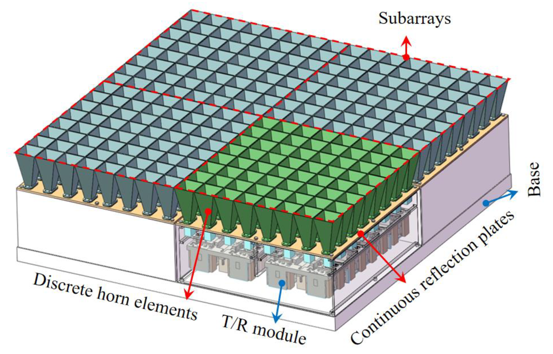
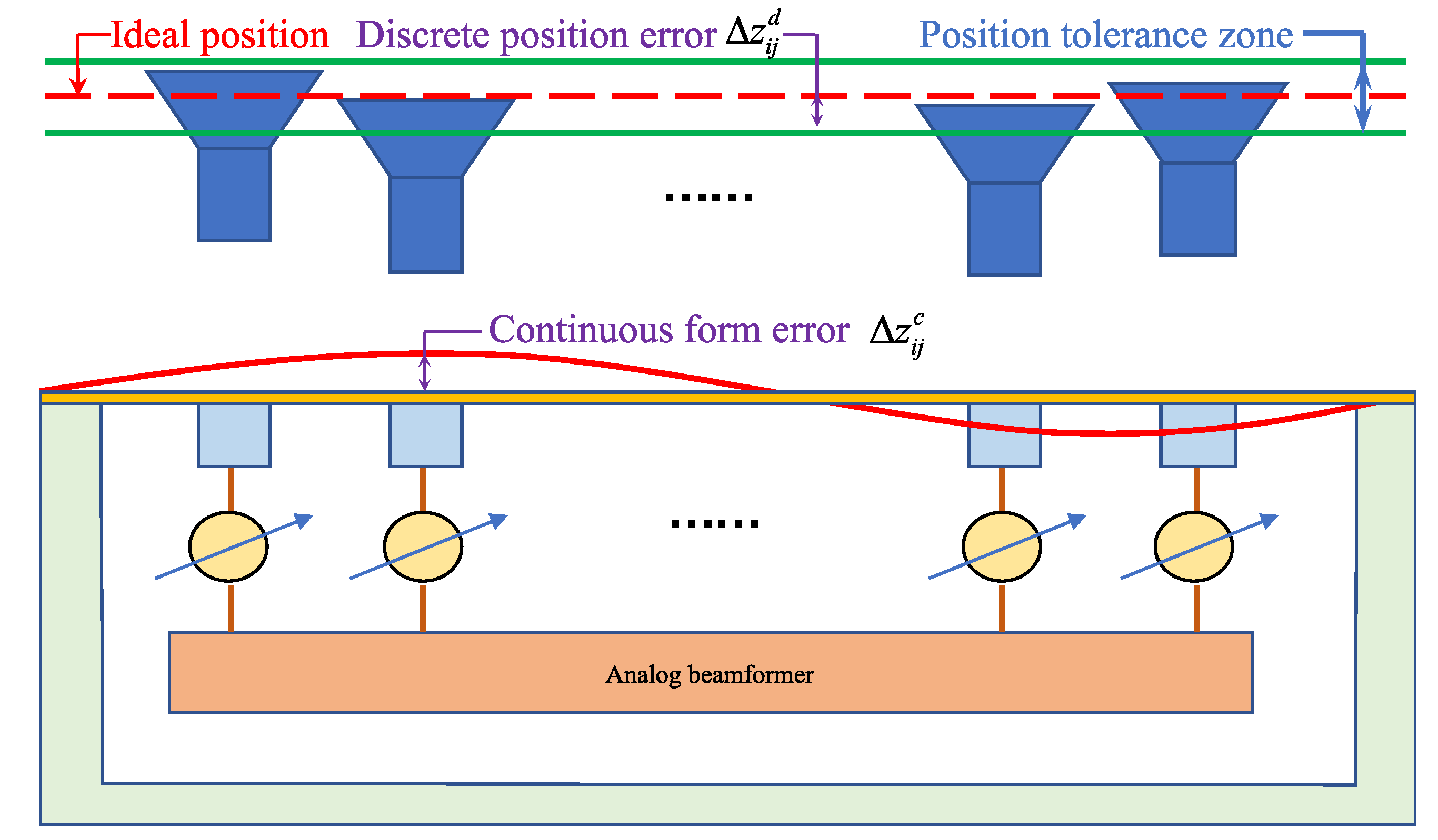
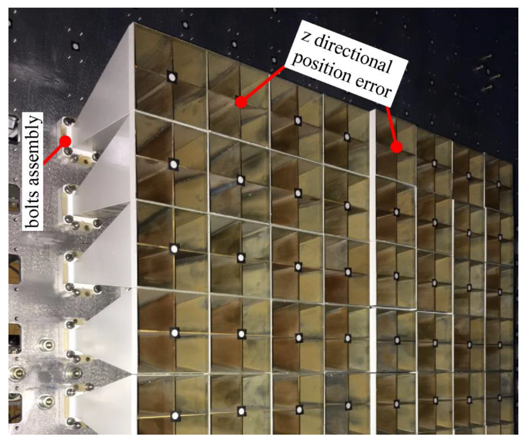
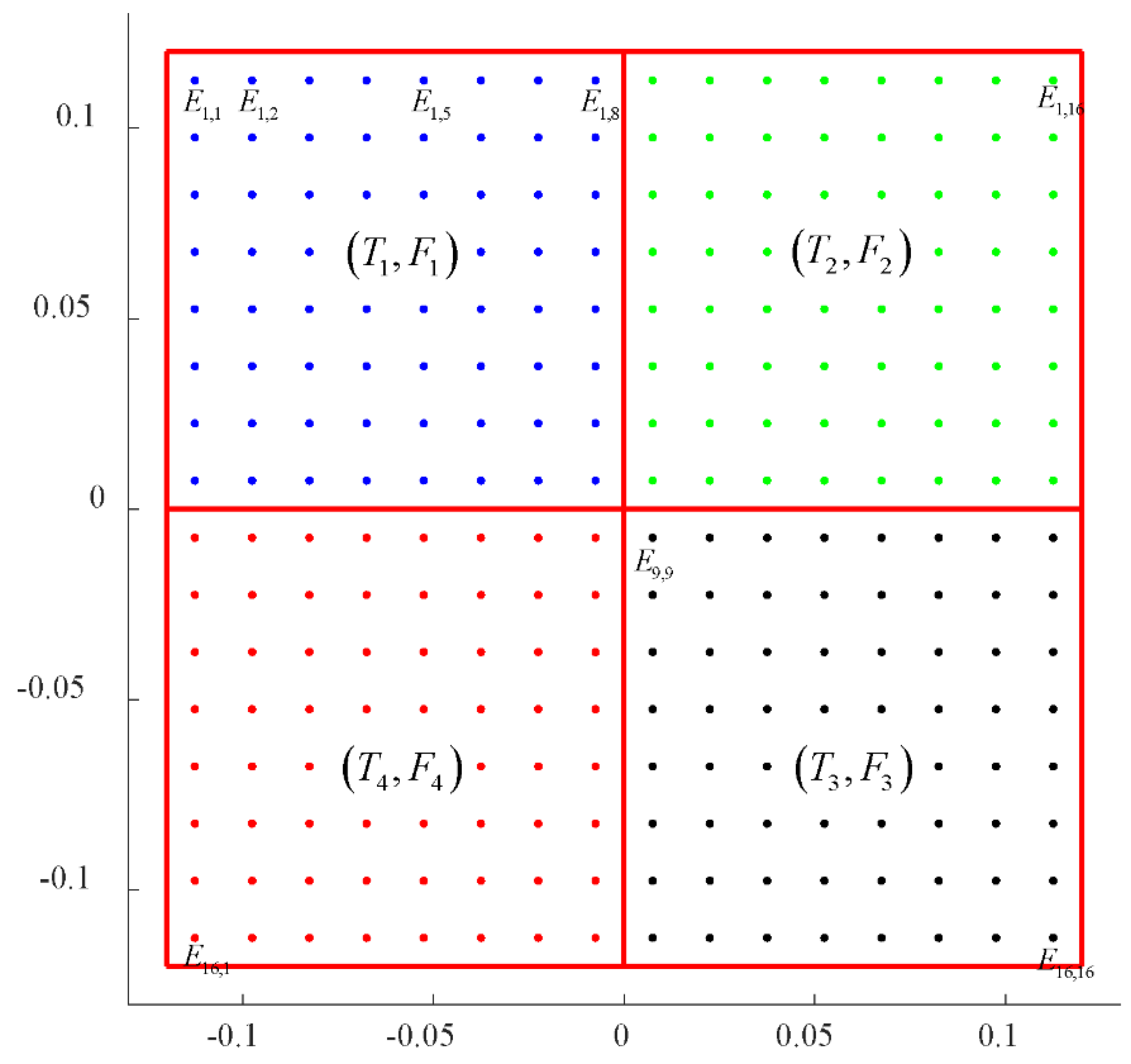
2.1. Hybrid Error Analysis

Supposing the array antenna contains n elements in the x direction and m elements in the y direction. Then the hybrid position error of the elements is defined as Equation (1), as shown in Figure 3. Note that the x and y directional position error was ignored, because they can hardly affect the main beam and the first side lobe [15], which reflects the performance of the antenna, and details of this can be found in Appendix A. The influences of x and y directional position errors were ignored, and several researchers have also adopted this approximation [2,15,17].

$$\Delta z_{ij}=\Delta z_{ij}^d+\Delta z_{ij}^c,i=1,2,\cdots m,j=1,2,\cdots n$$

(1)

The horns were bolted to the reflection plate, the position (especially the z directional position) of the horn elements is affected by the manufacture error and assembly deformation, as shown in Figure 4.

The discrete errors $\Delta z_{ij}^d$ are independent of each other, and they are assumed as a normally distributed variable.

$$\Delta z_{ij}^d~N\left(0,{\left({\sigma }_{ij}^d\right)}^2\right)$$

(2)

For elements in the same subarray, the distribution parameters are the same naturally. Because the position tolerance T of elements in the subarray is the same, the standard deviation is defined as based on the 3-sigma theory:

$${\sigma }_{ij}^d=\frac{1}{6}T$$

(3)

The continuous errors in the z direction are mutual dependent, they are assumed as multi-dimensional normally distributed variables, where the expectations equal zero and the covariance matrix $\Theta$ is determined by the manufacturer.

$$\begin{array}{l}\left\{\Delta z_{1,1}^c,\cdots \Delta z_{ij}^c,\cdots \Delta z_{mn}^c\right\}\sim N_{m\times n}\left({\mu }_c,\Theta \right), {\mu }_c=\left[0,0,\cdots ,0\right]\\ \Theta =\left[\begin{array}{ccccc}{\left({\sigma }_{1,1}^c\right)}^2& \cdots & cov\left(\Delta z_{1,1}^c,\Delta z_{ij}^c\right)& \cdots & cov\left(\Delta z_{1,1}^c,\Delta z_{mn}^c\right)\\ ⋮& \ddots & ⋮& \ddots & ⋮\\ cov\left(\Delta z_{ij}^c,\Delta z_{1,1}^c\right)& \cdots & {\left({\sigma }_{ij}^c\right)}^2& \cdots & cov\left(\Delta z_{ij}^c,\Delta z_{mn}^c\right)\\ ⋮& \ddots & ⋮& \ddots & ⋮\\ cov\left(\Delta z_{mn}^c,\Delta z_{1,1}^c\right)& \cdots & cov\left(\Delta z_{mn}^c,\Delta z_{ij}^c\right)& \cdots & {\left({\sigma }_{mn}^c\right)}^2\end{array}\right]\end{array}$$

(4)

The covariance matrix is determined by the flatness of the reflection plate, which is estimated based on the measured data, and details can be found in our previous work [18].

$$\Theta =\psi \left(F\right)$$

(5)

Since the discrete error and continuous error are mutual independent, then the hybrid error $\Delta z_{ij}$ is a normally distributed variable. The expectation and variance can be determined directly as follows:

$$\begin{array}{l}E\left(\Delta z_{ij}\right)=E\left(\Delta z_{ij}^d\right)+E\left(\Delta z_{ij}^c\right)=0\\ D\left(\Delta z_{ij}\right)=D\left(\Delta z_{ij}^d\right)+D\left(\Delta z_{ij}^c\right)={\left({\sigma }_{ij}^d\right)}^2+{\left({\sigma }_{ij}^c\right)}^2\\ cov\left(\Delta z_{ij},\Delta z_{pq}\right)=cov\left(\Delta z_{ij}^c,\Delta z_{pq}^c\right),ij\ne pq\end{array}$$

(6)

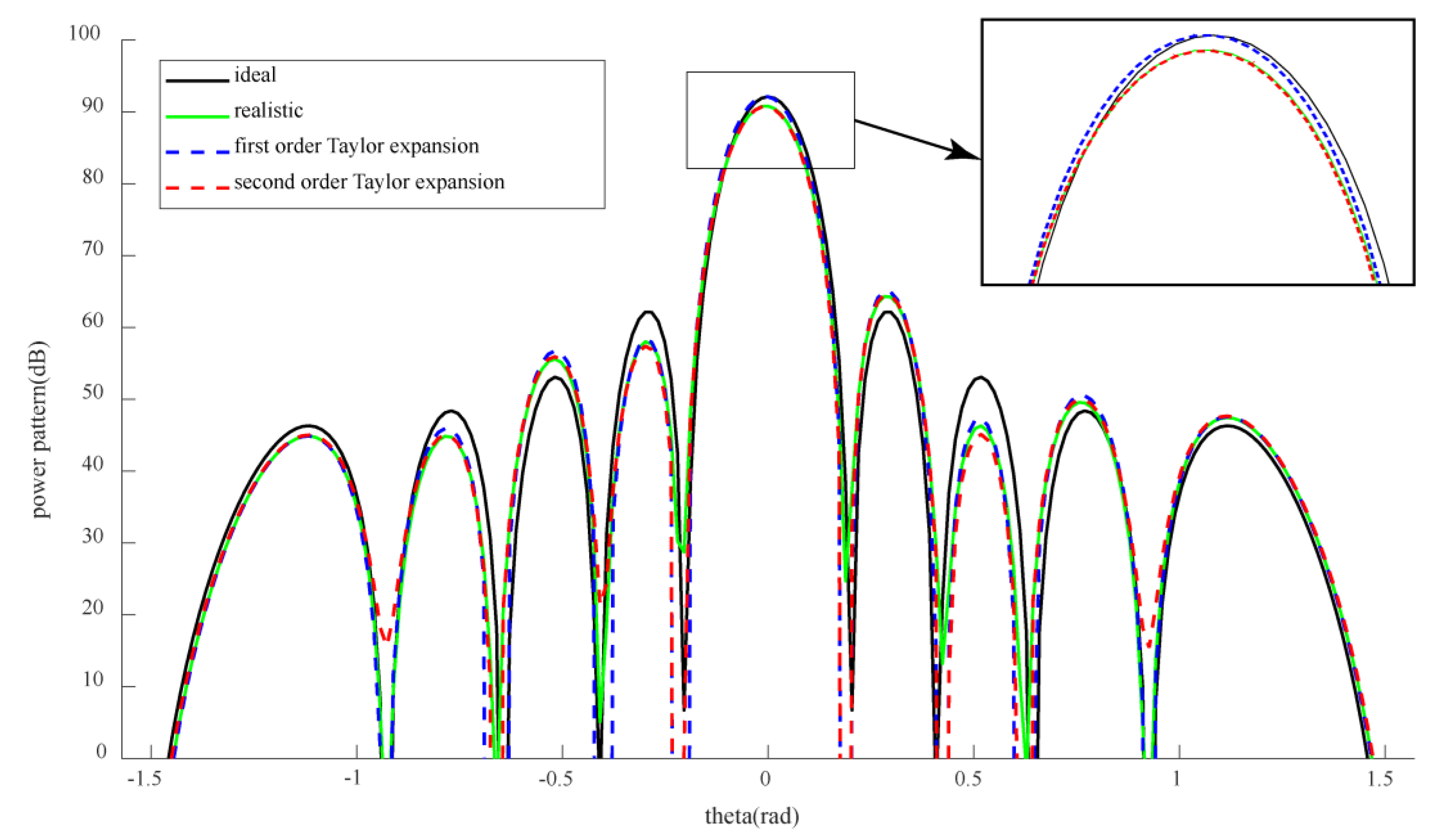
2.2. Second-Order Taylor Expansion

The gain of the antenna cannot be used to optimize the tolerance directly, because the realistic gain of the antenna cannot be modeled explicitly in a statistical way, and details can be found in Appendix C. The power pattern was used to optimize the tolerances in this paper instead, as shown in Figure 5. The correlation function between the antenna power pattern and the position errors of the elements has been established based on the first-order Taylor expansion in our previous work [16].

$$P\left(\theta ,\phi \right)\approx P_o+{\displaystyle \sum }_{i=1}^m{\displaystyle \sum }_{j=1}^n\left\{\frac{\partial P}{\partial x_{ij}}\Delta x_{ij}+\frac{\partial P}{\partial y_{ij}}\Delta y_{ij}+\frac{\partial P}{\partial z_{ij}}\Delta z_{ij}\right\}$$

(7)

where $P\left(\theta ,\phi \right)$ represents the realistic power pattern of the antenna, and $P_o$ represents the ideal power pattern. For the convenience of description, $P\left(\theta ,\phi \right)$ is abbreviated as $P$ in the following.

The far field patterns of all the horn antennas are assumed to be the same, and the far-field pattern of the horn is assumed as ideal. Based on the above assumption, the far-field patterns of the horns are just coefficients used to multiply the array factor, the pattern of the array antenna is affected only by the array factor. The main lobe becomes sharp if considering the far-field pattern of the horn. In order to show the changes of the array factor more clearly, the far-field pattern of the horn is not considered.

The maximum power density in the main lobe reflects the detection capability of the antenna and was used to optimize the hybrid tolerances. The side lobes in the power pattern are not important in our analysis.

To improve the approximation precision of the performance, the second-order Taylor expansion was derived, as shown in Equation (8). Details can be found in Appendix A.

$$P\left(\theta ,\phi \right)\approx P_o+{\displaystyle \sum }_{i=1}^m{\displaystyle \sum }_{j=1}^n\left\{\frac{\partial P}{\partial z_{ij}}\Delta z_{ij}\right\}+\frac{1}{2}{\displaystyle \sum }_{i=1}^m{\displaystyle \sum }_{j=1}^n\left\{\frac{{\partial }^{2}P}{\partial z_{ij}^2}\Delta z_{ij}^2\right\}=P_o+\Delta P$$

(8)

For the convenience of expression, Equation (8) was rewritten as follow.

$$\Delta P\approx \Delta P_1+\Delta P_2, \Delta P_1={\displaystyle \sum }_{i=1}^m{\displaystyle \sum }_{j=1}^n\left\{\frac{\partial P}{\partial z_{ij}}\Delta z_{ij}\right\}, \Delta P_2=\frac{1}{2}{\displaystyle \sum }_{i=1}^m{\displaystyle \sum }_{j=1}^n\left\{\frac{{\partial }^{2}P}{\partial z_{ij}^2}\Delta z_{ij}^2\right\}$$

(9)

To illustrate the effectiveness, the second-order Taylor expansion was applied to the $8\times 8$ subarray with random geometric errors, as shown in Figure 6. In the main lobe, the second-order Taylor expansion is much more precise than the first-order Taylor expansion, and in the side lobes, the second-order Taylor expansion is almost same with the first-order Taylor expansion.

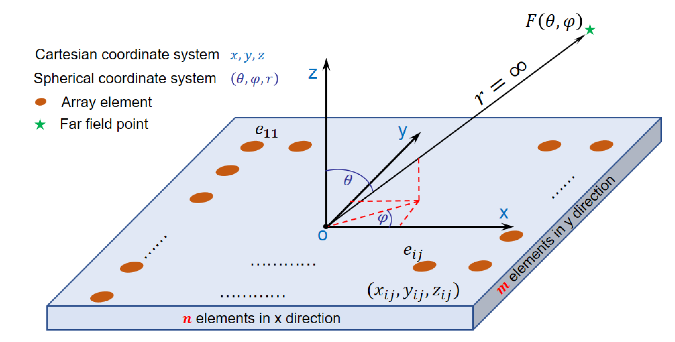
3. Statistical Analysis of the Performance of the Array Antenna

Based on the Lyapunov’s theorem (Appendix B), the deviation $\Delta P$ of the performance approximately obeys normal distribution, because the array antenna is composed of a large number of elements. For example, an active-phased array ballistic missile detection antenna in America has more than 2600 elements [19].

$$\Delta P\sim N\left(\mu ,{\sigma }^2\right)$$

(10)

3.1. Expectation Derivation

The expectation of the maximum power density deviation $\Delta P$ is determined as follows based on the mathematical definition.

$$\mu =E\left(\Delta P_1+\Delta P_2\right)$$

(11)

$$\mu =E\left(\Delta P_1+\Delta P_2\right)$$

(12)

$$\begin{array}{c}E\left(\Delta P_2\right)=\frac{1}{2}E\left({\displaystyle \sum }_{i=1}^m{\displaystyle \sum }_{j=1}^n\left\{\frac{{\partial }^{2}P}{\partial z_{ij}^2}\Delta z_{ij}^2\right\}\right)=\frac{1}{2}{\displaystyle \sum }_{i=1}^m{\displaystyle \sum }_{j=1}^{n}E\left(\frac{{\partial }^{2}P}{\partial z_{ij}^2}\Delta z_{ij}^2\right)\\ =\frac{1}{2}{\displaystyle \sum }_{i=1}^m{\displaystyle \sum }_{j=1}^n\left\{\frac{{\partial }^{2}P}{\partial z_{ij}^2}E\left(\Delta z_{ij}^2\right)\right\}\end{array}$$

(13)

Based on the definition of variance, one can derive that:

$$D\left(\Delta z_{ij}\right)=E\left(\Delta z_{ij}^2\right)-{\left[E\left(\Delta z_{ij}\right)\right]}^2$$

(14)

Then the expectation of $\Delta z_{ij}^2$ can be determined:

$$E\left(\Delta z_{ij}^2\right)=D\left(\Delta z_{ij}\right)+{\left[E\left(\Delta z_{ij}\right)\right]}^2=\left[{\left({\sigma }_{ij}^d\right)}^2+{\left({\sigma }_{ij}^c\right)}^2\right]+{\left({\mu }_{ij}^d+{\mu }_{ij}^c\right)}^2={\left({\sigma }_{ij}^d\right)}^2+{\left({\sigma }_{ij}^c\right)}^2$$

(15)

Then the expectation of deviation $\Delta P$ is determined:

$$E\left(\Delta P_2\right)=\frac{1}{2}{\displaystyle \sum }_{i=1}^m{\displaystyle \sum }_{j=1}^n\left\{\frac{{\partial }^{2}P}{\partial z_{ij}^2}\left[{\left({\sigma }_{ij}^d\right)}^2+{\left({\sigma }_{ij}^c\right)}^2\right]\right\}$$

(16)

Finally, the expectation of deviation $\Delta P$ is determined:

$$\mu =E\left(\Delta P\right)=\frac{1}{2}{\displaystyle \sum }_{i=1}^m{\displaystyle \sum }_{j=1}^n\left\{\frac{{\partial }^{2}P}{\partial z_{ij}^2}\left[{\left({\sigma }_{ij}^d\right)}^2+{\left({\sigma }_{ij}^c\right)}^2\right]\right\}$$

(17)

3.2. Variance Derivation

The variance of the maximum power density deviation $\Delta P$ is defined as follows:

$$\begin{array}{ll}{\sigma }^2& =D\left(\Delta P_1+\Delta P_2\right)\\ & =D\left(\Delta P_1\right)+D\left(\Delta P_2\right)+2\mathrm{cov}\left(\Delta P_1,\Delta P_2\right)\end{array}$$

(18)

Based on the independence of the discrete error $z_{ij}^d$ and continuous error $z_{ij}^c$, the variance of $D\left(\Delta P_1\right)$ can be derived as follows:

$$\begin{array}{cc}\hfill D\left(\Delta P_1\right)& =D\left({\displaystyle \sum _{i=1}^m{\displaystyle \sum _{j=1}^n\left\{\frac{\partial P}{\partial z_{ij}}\left(\Delta z_{ij}^d+\Delta z_{ij}^c\right)\right\}}}\right)\hfill \\ & =D\left({\displaystyle \sum _{i=1}^m{\displaystyle \sum _{j=1}^n\left\{\frac{\partial P}{\partial z_{ij}}\Delta z_{ij}^d\right\}+{\displaystyle \sum _{i=1}^m{\displaystyle \sum _{j=1}^n\left\{\frac{\partial P}{\partial z_{ij}}\Delta z_{ij}^c\right\}}}}}\right)\hfill \\ & =D\left({\displaystyle \sum _{i=1}^m{\displaystyle \sum _{j=1}^n\left\{\frac{\partial P}{\partial z_{ij}}\Delta z_{ij}^d\right\}}}\right)+D\left({\displaystyle \sum _{i=1}^m{\displaystyle \sum _{j=1}^n\left\{\frac{\partial P}{\partial z_{ij}}\Delta z_{ij}^c\right\}}}\right)\hfill \\ & ={\displaystyle \sum _{i=1}^m{\displaystyle \sum _{j=1}^n\left\{{\left(\frac{\partial P}{\partial z_{ij}}\right)}^2\left[D\left(\Delta z_{ij}^d\right)+D\left(\Delta z_{ij}^c\right)\right]\right\}}}+\frac{1}{2}{\displaystyle \sum _{i=1}^m{\displaystyle \sum _{j=1}^n{\displaystyle \sum _{\begin{array}{l}p=1\\ ij\ne pq\end{array}}^m{\displaystyle \sum _{q=1}^n\frac{\partial P}{\partial z_{ij}}}}}\cdot \frac{\partial P}{\partial z_{pq}}\cdot \mathrm{cov}\left(\Delta z_{ij}^c,\Delta z_{pq}^c\right)}\hfill \\ & ={\displaystyle \sum _{i=1}^m{\displaystyle \sum _{j=1}^n\left\{{\left(\frac{\partial P}{\partial z_{ij}}\right)}^2\left[{\left({\sigma }_{ij}^d\right)}^2+{\left({\sigma }_{ij}^c\right)}^2\right]\right\}}}+\frac{1}{2}{\displaystyle \sum _{i=1}^m{\displaystyle \sum _{j=1}^n{\displaystyle \sum _{\begin{array}{l}p=1\\ ij\ne pq\end{array}}^m{\displaystyle \sum _{q=1}^n\frac{\partial P}{\partial z_{ij}}}}}\cdot \frac{\partial P}{\partial z_{pq}}\cdot \mathrm{cov}\left(\Delta z_{ij}^c,\Delta z_{pq}^c\right)}\hfill \end{array}$$

(19)

The variance of $D\left(\Delta P_2\right)$ can be derived as follows:

$$\begin{array}{ll}D\left(\Delta P_2\right)& =\frac{1}{4}D\left({\displaystyle \sum _{i=1}^m{\displaystyle \sum _{j=1}^n\left\{\frac{{\partial }^{2}P}{\partial z_{ij}^2}\Delta z_{ij}^2\right\}}}\right)\\ & =\frac{1}{4}\left\{{\displaystyle \sum _{i=1}^m{\displaystyle \sum _{j=1}^n\left[{\left(\frac{{\partial }^{2}P}{\partial z_{ij}^2}\right)}^{2}D\left(\Delta z_{ij}^2\right)\right]}}+2{\displaystyle \sum _{i=1}^m{\displaystyle \sum _{j=1}^n{\displaystyle \sum _{\begin{array}{l}p=1\\ ij\ne pq\end{array}}^m{\displaystyle \sum _{q=1}^n\frac{{\partial }^{2}P}{\partial z_{ij}^2}}}}\cdot \frac{{\partial }^{2}P}{\partial z_{pq}^2}\cdot \mathrm{cov}\left(\Delta z_{ij}^2,\Delta z_{pq}^2\right)}\right\}\end{array}$$

(20)

Based on the conclusion in Appendix C, $\Delta z_{ij}^2$ obeys Gamma distribution and the variance is:

$$D\left(\Delta z_{ij}^2\right)=2{\left({\left({\sigma }_{ij}^d\right)}^2+{\left({\sigma }_{ij}^c\right)}^2\right)}^2$$

(21)

According to the mathematical definition, the covariance is expanded as follows:

$$cov\left(\Delta P_1,\Delta P_2\right)=E\left(\Delta P_1\cdot \Delta P_2\right)-E\left(\Delta P_1\right)E\left(\Delta P_2\right)$$

(22)

For the convenience of description, part of $\Delta P_1$ and $\Delta P_2$ are abbreviated as $A_{ij}$ and $B_{ij}$.

$$A_{ij}=\frac{\partial P}{\partial z_{ij}}\Delta z_{ij}, B_{ij}=\frac{1}{2}\frac{{\partial }^{2}P}{\partial z_{ij}^2}\Delta z_{ij}^2$$

(23)

Expanding the $\Delta P_1\cdot \Delta P_2$ as the sum of polynomials:

$$\begin{array}{ll}\Delta P_1\cdot \Delta P_2=& \left\{\begin{array}{ccccccc}{A}_{11}{B}_{11}& +& A_{11}{B}_{12}& +& \cdots & +& A_{11}{B}_{mn}\\ +A_{12}{B}_{11}& +& A_{12}{B}_{12}& +& \cdots & +& A_{12}{B}_{mn}\\ ⋮& & ⋮& & \ddots & & ⋮\\ +A_{1n}{B}_{11}& +& A_{1n}{B}_{12}& +& \cdots & +& A_{1n}{B}_{mn}\end{array}\right\}+\cdots \\ & \hspace{1em}+\left\{\begin{array}{ccccccc}{A}_{m1}{B}_{11}& +& A_{m1}{B}_{12}& +& \cdots & +& A_{m1}{B}_{mn}\\ +A_{m2}{B}_{11}& +& A_{m2}{B}_{12}& +& \cdots & +& A_{m2}{B}_{mn}\\ ⋮& & ⋮& & \ddots & & ⋮\\ +A_{mn}{B}_{11}& +& A_{mn}{B}_{12}& +& \cdots & +& A_{mn}{B}_{mn}\end{array}\right\}\end{array}$$

(24)

As shown in Equation (12) that $E\left(\Delta P_1\right)=0$, then Equation (22) can be rewritten as:

$$cov\left(\Delta P_1,\Delta P_2\right)={\displaystyle \sum }_{i=1}^m{\displaystyle \sum }_{j=1}^n{\displaystyle \sum }_{p=1}^m{\displaystyle \sum }_{q=1}^n\left\{E\left(A_{ij}{B}_{pq}\right)\right\}$$

(25)

where

$$E\left(A_{ij}{B}_{pq}\right)=\frac{1}{2}\frac{\partial P}{\partial z_{ij}}\frac{{\partial }^{2}P}{\partial z_{pq}^2}E\left(\Delta z_{ij}\cdot \Delta z_{pq}^2\right)$$

(26)

Due to the symmetry of the probability density function (the normal distribution with ${\mu }_{ij}=0$), the expectation is zero.

$$E\left(\Delta z_{ij}\cdot \Delta z_{pq}^2\right)=0\Rightarrow E\left(A_{ij}{B}_{pq}\right)=0$$

(27)

Then the covariance is derived as Equation (22):

$$cov\left(\Delta P_1,\Delta P_2\right)=0$$

(28)

Finally, the variance of the deviation $\Delta P$ of the performance is determined:

$$\begin{array}{ll}{\sigma }^2& =D\left(\Delta P\right)\\ & ={\displaystyle \sum _{i=1}^m{\displaystyle \sum _{j=1}^n\left\{{\left(\frac{\partial P}{\partial z_{ij}}\right)}^2\left[{\left({\sigma }_{ij}^d\right)}^2+{\left({\sigma }_{ij}^c\right)}^2\right]\right\}}}+\frac{1}{2}{\displaystyle \sum _{i=1}^m{\displaystyle \sum _{j=1}^n{\displaystyle \sum _{\begin{array}{l}p=1\\ ij\ne pq\end{array}}^m{\displaystyle \sum _{q=1}^n\frac{\partial P}{\partial z_{ij}}}}}\cdot \frac{\partial P}{\partial z_{pq}}\cdot \mathrm{cov}\left(\Delta z_{ij}^c,\Delta z_{pq}^c\right)}\\ & +\frac{1}{2}\left\{{\displaystyle \sum _{i=1}^m{\displaystyle \sum _{j=1}^n\left[{\left(\frac{{\partial }^{2}P}{\partial z_{ij}^2}\right)}^2\cdot {\left({\left({\sigma }_{ij}^d\right)}^2+{\left({\sigma }_{ij}^c\right)}^2\right)}^2\right]}}+{\displaystyle \sum _{i=1}^m{\displaystyle \sum _{j=1}^n{\displaystyle \sum _{\begin{array}{l}p=1\\ ij\ne pq\end{array}}^m{\displaystyle \sum _{q=1}^n\frac{{\partial }^{2}P}{\partial z_{ij}^2}}}}\cdot \frac{{\partial }^{2}P}{\partial z_{pq}^2}\cdot \mathrm{cov}\left(\Delta z_{ij}^2,\Delta z_{pq}^2\right)}\right\}\end{array}$$

(29)

The variance is determined by the standard deviation of the geometric error and the covariance. The covariance matrix is determined by the manufacturer, not by the tolerance. Therefore, the terms containing covariance are recorded as constant C(F). Noticing that for any given array antenna, C(F) is totally defined by the flatness F of the reflection plate.

$$\begin{array}{ll}{\sigma }^2=D\left(\Delta P\right)=& {\displaystyle \sum }_{i=1}^m{\displaystyle \sum }_{j=1}^n\left\{{\left(\frac{\partial P}{\partial z_{ij}}\right)}^2\left[{\left({\sigma }_{ij}^d\right)}^2+{\left({\sigma }_{ij}^c\right)}^2\right]\right\}\\ & \hspace{1em}+\frac{1}{2}{\displaystyle \sum }_{i=1}^m{\displaystyle \sum }_{j=1}^n\left[{\left(\frac{{\partial }^{2}P}{\partial z_{ij}^2}\right)}^2\cdot {\left({\left({\sigma }_{ij}^d\right)}^2+{\left({\sigma }_{ij}^c\right)}^2\right)}^2\right]+C\left(F\right)\end{array}$$

(30)

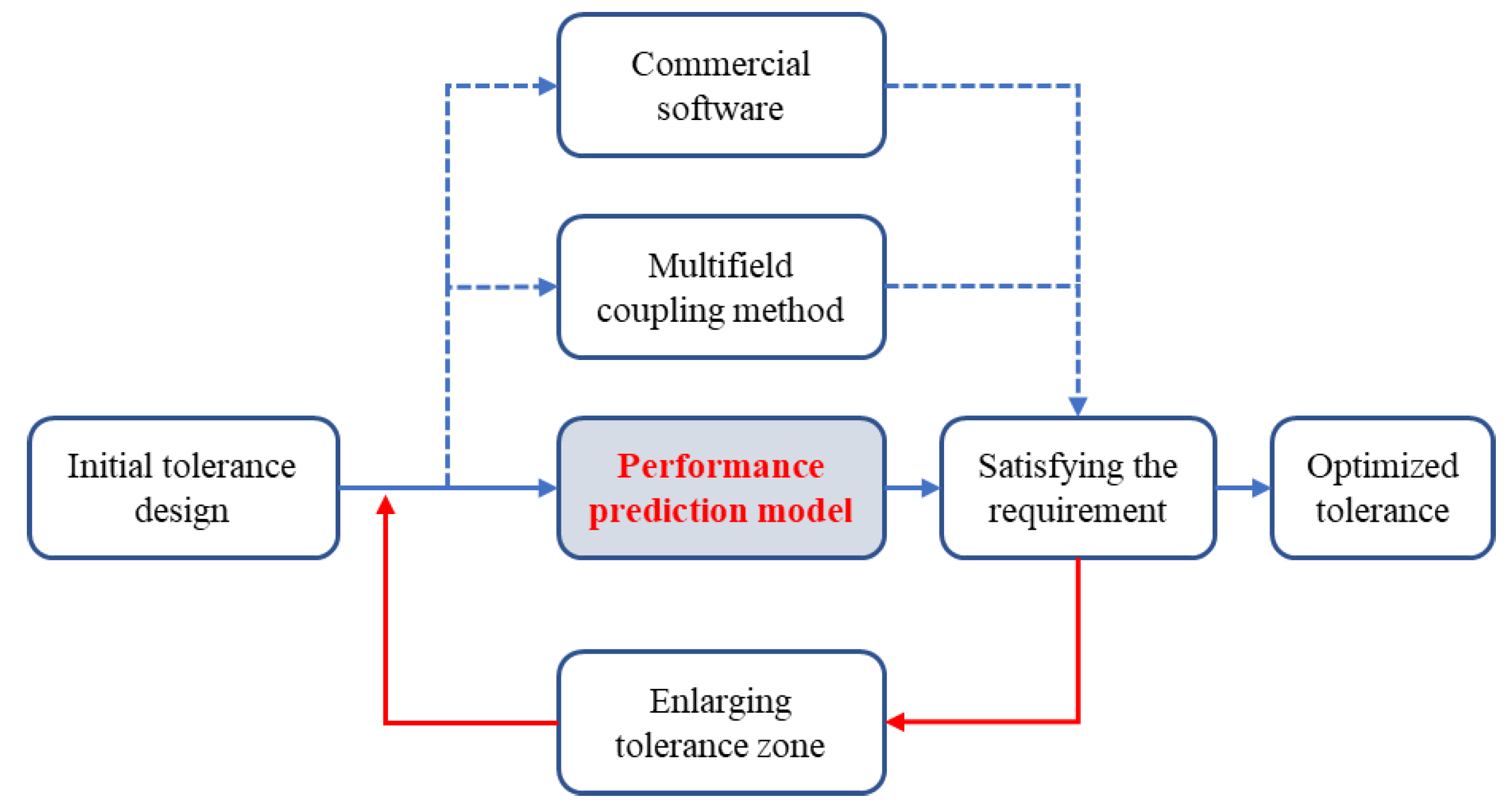
4. Tolerance Design Based on the Statistical Model

Based on the statistical analysis (Equations (17) and (30)), the position tolerance of the discrete elements and the flatness of the continuous reflection plate can be optimized simultaneously.

Equations (3) and (5) describe the relation between the standard deviation of the geometric error and the tolerance. The tolerance optimization model was defined as follows:

$$\begin{array}{l}max P_0\left(\theta ,\phi \right)+\mu \left(\theta ,\phi \right)-3\sigma \left(\theta ,\phi \right)\\ s.t.T\in \left[T_{min},T_{max}\right], {\sigma }_{ij}^d=\frac{1}{6}T\\ F\in \left[F_{min},F_{max}\right],{\sigma }_{ij}^c=\frac{1}{6}F\\ g\left(T,F\right)\le g_0\end{array}$$

(31)

where the $\left(\mu -3\sigma \right)$ represents the lower boundary of the interval of the power pattern, as shown in Figure 7. The $g\left(T,F\right)$ represents the cost of manufacture, which is defined by the exponential model [20,21]:

$$g\left(T,F\right)={\displaystyle \sum }_{v=1}^V\left[e^{-T}+\left(0.15+e^{-2F}\right)\right]$$

(32)

The position tolerance $T$ of the discrete elements is constrained by $\left[T_{min},T_{max}\right]$, the flatness $F$ of the plate is constrained by $\left[F_{min},F_{max}\right]$. The lower bound $T_{min}$ and $F_{min}$ is restricted by the manufacturer, and the upper bound $T_{max}$ and $F_{max}$ is constrained by the assembly.

Due to the hybrid errors of the antenna, the realistic maximum power density is always smaller than the ideal maximum power density, and the interval of the power pattern is illustrated in Figure 6. The red curve represents the upper bound, the blue curve represents the lower bound, and the black curve represents the ideal power pattern. The interval enclosed by the red curve and blue curve indicates that 99.7% of the possible realistic results fall within:

$$\left[P_0+\mu -3\sigma ,P_0+\mu +3\sigma \right]$$

(33)

The maximum power density locates on the angle $\left(\theta ,\phi \right)=\left(0,0\right)$. Equation (31) can be solved by the feasible direction method.

5. Results

The proposed hybrid tolerance design method was applied to a spaceborne active phased array antenna. The CAD model is shown in Figure 1. The array antenna is assembled from 4 subarrays, each subarray is composed of $8\times 8=64$ horn elements. The operating wavelength is $\lambda =30 \mathrm{mm}$, and the element spacing is $d=0.5\lambda =15 \mathrm{mm}$. The initial phase of each element is set as zero and the amplitude of each element is set as one. All the elements are numbered as shown in Figure 8.

The first-order derivation and second-order derivation in $\left(\theta ,\phi \right)=\left(0,0\right)$ were calculated according to Equations (A6) and (A7), since all the amplitudes are set as one, and then all the second order derivatives are the same.

$$\frac{\partial P\left(0,0\right)}{\partial z_{ij}}=0,\frac{{\partial }^{2}P\left(\theta ,\phi \right)}{\partial z_{ij}^2}=-5.5270\mathrm{e}+06$$

(34)

Due to the symmetry of the array antenna, all the tolerances of each subarray are the same:

$$F_1=F_2=F_3=F_4=F; T_1=T_2=T_3=T_4=T$$

(35)

The interval prediction (Equation (33)) was validated through 1000 sets of simulations on the whole array antenna. Simulation results show that the variation range of the power pattern based on Equations (17) and (30) was very accurate, and the experimental results showed that 996 results of 1000 total experiments satisfied the predicted fluctuation interval, as shown in Figure 9.

The flatness of the reflection plate was discretized to 6 specific values, that is:

$$F=\left\{\frac{1}{60}\lambda ,\frac{1}{30}\lambda ,\frac{1}{20}\lambda ,\frac{1}{15}\lambda ,\frac{1}{12}\lambda ,\frac{1}{10}\lambda \right\}$$

(36)

The covariance matrix $\Theta$ of $\left\{\Delta z_{11}^c,\cdots \Delta z_{ij}^c,\cdots \Delta z_{88}^c\right\}$ for each flatness of reflection plate of the subarray was estimated. For example, the covariance matrix corresponding to $F=0.1\lambda$ was shown in Figure 10. The diagonal elements represent the variance ${\left({\sigma }_{ij}^c\right)}^2$ and the rest represent the covariance $cov\left(\Delta z_{ij}^c,\Delta z_{pq}^c\right)$.

Obviously, the values of the diagonal elements of the covariance matrix are much bigger than those of the rest, which indicates the correlation between continuous errors of adjacent assembly holes on the reflection plate. For example:

$$cov\left(\Delta z_{1,1}^c,\Delta z_{1,2}^c\right)\gg cov\left(\Delta z_{1,1}^c,\Delta z_{3,5}^c\right)$$

(37)

The 4 subarrays are independent of each other, and they have the same tolerances. Therefore, the covariance matrix $\Sigma$ of the whole array can be determined easily based on the covariance matrix $\Theta$ of the subarray plate.

$$\Sigma =\left[\begin{array}{cccc}\Theta & \mathbf{0}& \mathbf{0}& \mathbf{0}\\ \mathbf{0}& \Theta & \mathbf{0}& \mathbf{0}\\ \mathbf{0}& \mathbf{0}& \Theta & \mathbf{0}\\ \mathbf{0}& \mathbf{0}& \mathbf{0}& \Theta \end{array}\right]$$

(38)

where $\Sigma$ is block matrix and $\mathbf{0}$ represents the zero matrix.

The highest tolerance cost was set as $g_0=0.35$ for the spaceborne active phased-array antenna in Equation (32), then the feasible solutions of the hybrid tolerances were constrained in the area enclosed by the red line in Figure 11.

The expectation of the $\Delta P\left(0,0\right)$ for different position tolerance $T$ and flatness F was calculated based on Equations (17) and (30), as shown in Figure 12a and

Table 1. The expectation of the maximum power density degradation.

Expectation (db) $-\mathit{E}\left(\mathit{\Delta }\mathit{P}\right)$		Flatness of the Reflection Plate (mm)
		0.5	1.0	1.5	2.0	2.5	3.0
Position tolerance of the discrete elements (mm)	0.50	0.0232	0.0768	0.1649	0.2930	0.4534	0.6562
	0.75	0.0298	0.0834	0.1716	0.2997	0.4602	0.6630
	1.00	0.0390	0.0927	0.1809	0.3091	0.4696	0.6726
	1.25	0.0509	0.1046	0.1929	0.3212	0.4818	0.6850
	1.50	0.0655	0.1192	0.2076	0.3359	0.4967	0.7001
	1.75	0.0827	0.1364	0.2249	0.3534	0.5144	0.7179
	2.00	0.1025	0.1564	0.2449	0.3736	0.5347	0.7385
	2.25	0.1251	0.1790	0.2677	0.3965	0.5579	0.7619
	2.50	0.1503	0.2043	0.2931	0.4221	0.5837	0.7881
	2.75	0.1783	0.2323	0.3213	0.4505	0.6124	0.8171
	3.00	0.2089	0.2631	0.3522	0.4816	0.6438	0.8489

. The standard deviation was calculated as shown in

Table 2. The standard deviation of the maximum power density degradation.

Standard Deviation $\sqrt{\mathit{D}\left(\mathit{\Delta }\mathit{P}\right)} \left(\mathbf{db}\right)$		Flatness of the Reflection Plate (mm)
		0.5	1.0	1.5	2.0	2.5	3.0
Position tolerance of the discrete elements (mm)	0.50	0.0030	0.0119	0.0268	0.0478	0.0727	0.1091
	0.75	0.0031	0.0120	0.0268	0.0479	0.0728	0.1093
	1.00	0.0033	0.0121	0.0270	0.0480	0.0730	0.1094
	1.25	0.0036	0.0123	0.0272	0.0482	0.0732	0.1097
	1.50	0.0040	0.0126	0.0274	0.0485	0.0735	0.1100
	1.75	0.0046	0.0130	0.0277	0.0488	0.0738	0.1103
	2.00	0.0053	0.0134	0.0281	0.0491	0.0741	0.1107
	2.25	0.0062	0.0140	0.0285	0.0495	0.0746	0.1112
	2.50	0.0072	0.0146	0.0290	0.0500	0.0751	0.1117
	2.75	0.0084	0.0155	0.0297	0.0506	0.0757	0.1123
	3.00	0.0097	0.0164	0.0304	0.0512	0.0763	0.1130

. Results shows that the power pattern is more sensitive to the flatness than the position tolerance. The flatness of the reflection plate plays a more important role in the tolerance design than the position tolerance.

Finally, based on Equations (31) and (32), the position tolerance of the discrete elements and the flatness of the reflection plates were optimized, in the feasible area, the minimum degradation of the maximum power density locates on the point (T, F), where the flatness is F = 1.5 mm, and the position tolerance is T = 2 mm, as shown in Figure 12b. The corresponding maximum power density degradation is 0.25 dB and the standard deviation is 0.03 dB. The performance of the antenna was optimized under the constraint of tolerance cost.

For the optimized tolerances, the distribution parameters of the realistic gain were estimated by numerical simulation. In total, 1000 sets of samples of hybrid errors and corresponding gain were calculated, as shown in Figure 13. The expectation of the gain was 25.68 dB (ideal gain was 25.91 dB), and the standard deviation of the gain was 0.027 dB.

6. Conclusions

A hybrid tolerance design method was proposed in this paper, and the position tolerance of the discrete elements and the flatness of the continuous reflection plate were optimized simultaneously.

• The hybrid geometric errors of the array antenna were analyzed, and the surrogate model of the electrical performance and hybrid geometric errors were established based on the second-order Taylor expansion.
• The expectation and the variance of the power pattern of the array antenna was derived, then the direct and explicit relationship between the performance and the hybrid tolerances was identified.
• The proposed method was applied on an active phased-array antenna, and the hybrid tolerances were optimized finally. Numerical simulation results prove the effectiveness of the method.

References

1. Elliott, R. Mechanical and Electrical Tolerances for Two-Dimensional Scanning Antenna Arrays. IRE Trans. Antennas Propag. 1958, 6, 114–120. [Google Scholar] [CrossRef]
2. Wang, H.S.C. Performance of phased-array antennas with mechanical errors. IEEE Trans. Aerosp. Electron. Syst. 1992, 28, 535–545. [Google Scholar] [CrossRef]
3. So, K.K.; Luk, K.M.; Chan, C.H.; Chan, K.F. 3D Printed High Gain Complementary Dipole/Slot Antenna Array. Appl. Sci. 2018, 8, 1410. [Google Scholar] [CrossRef] [Green Version]
4. Lee, H.; Kim, S.; Choi, J. A 28 GHz 5G Phased Array Antenna with Air-Hole Slots for Beam Width Enhancement. Appl. Sci. 2019, 9, 4204. [Google Scholar] [CrossRef] [Green Version]
5. Wang, C.; Yuan, S.; Yang, X.; Gao, W.; Zhu, C.; Wang, Z.; Wang, S.; Peng, X. Position Tolerance Design Method for Array Antenna in Internet of Things. Wirel. Commun. Mob. Comput. 2018, 2018, 1–6. [Google Scholar] [CrossRef] [Green Version]
6. Ruze, J. The Effect of Aperture Errors on the Antenna Radiation Pattern. Il Nuovo Cim. 1952, 9, 364–380. [Google Scholar] [CrossRef]
7. Bao, V.T. Influence of correlation interval and illumination taper in antenna tolerance theory. Proc. Inst. Electr. Eng. 1969, 116, 195. [Google Scholar] [CrossRef]
8. Rahmat-Samii, Y. An efficient computational method for characterizing the effects of random surface errors on the average power pattern of reflectors. IRE Trans. Antennas Propag. 1983, 31, 92–98. [Google Scholar] [CrossRef]
9. Kim, J.W.; Kim, B.S.; Nam, S.; Lee, C.W. Computation of the Average Power Pattern of a Reflector Antenna with Random Surface Errors and Misalignment Errors. IRE Trans. Antennas Propag. 1996, 44, 996–999. [Google Scholar] [CrossRef]
10. Lee, J.; Lee, Y.; Kim, H. Decision of error tolerance in array element by the Monte Carlo method. IRE Trans. Antennas Propag. 2005, 53, 1325–1331. [Google Scholar] [CrossRef]
11. Wang, C.; Kang, M.; Wang, W.; Zhong, J.; Zhang, Y.; Jiang, C.; Duan, B. Electromechanical coupling based performance evaluation of distorted phased array antennas with random position errors. Int. J. Appl. Electromagn. Mech. 2016, 51, 285–295. [Google Scholar] [CrossRef]
12. Schmid, C.M.; Schuster, S.; Feger, R.; Stelzer, A. On the effects of calibration errors and mutual coupling on the beam pattern of an antenna array. IRE Trans. Antennas Propag. 2013, 61, 4063–4072. [Google Scholar] [CrossRef]
13. Anselmi, N.; Manica, L.; Rocca, P.; Massa, A. Tolerance analysis of antenna arrays through interval arithmetic. IRE Trans. Antennas Propag. 2013, 61, 5496–5507. [Google Scholar] [CrossRef]
14. Anselmi, N.; Salucci, M.; Rocca, P.; Massa, A. Power pattern sensitivity to calibration errors and mutual coupling in linear arrays through circular interval arithmetics. Sensors 2016, 16, 791. [Google Scholar] [CrossRef]
15. Guo, F.; Liu, Z.; Sa, G.; Tan, J. A Position Error Representation Method for Planar Arrays. IEEE Antennas Wirel. Propag. Lett. 2019, 1. [Google Scholar] [CrossRef]
16. Sa, G.; Liu, Z.; Qiu, C.; Tan, J. A Novel Region-Division-Based Tolerance Design Method for a Large Number of Discrete Elements Distributed on a Large Surface. ASME J. Mech. Des. 2019, 141, 041701. [Google Scholar] [CrossRef]
17. Wang, C.; Duan, B.; Zhang, F.; Zhu, M. Analysis of performance of active phased array antennas with distorted plane error. Int. J. Electron. 2009, 96, 549–559. [Google Scholar] [CrossRef]
18. Sa, G.; Liu, Z.; Qiu, C.; Peng, X.; Tan, J. A Tolerance Analysis Method Considering Form Defects Based on Variance Separation. Proc. Inst. Mech. Eng. B J. Eng. Manuf. 2019, in press. [Google Scholar]
19. Winkler, D.F.; Webster, J.L. Searching the Skies: The Legacy of the United States Cold War Defense Radar Program (No. SR-97-78); Construction Engineering Research Lab (Army): Champaign, IL, USA, 1997. [Google Scholar]
20. Liu, S.G.; Jin, Q.; Liu, C.; Xie, R.J. Analytical method for optimal component tolerances based on manufacturing cost and quality loss. Proc. Inst. Mech. Eng. B J. Eng. Manuf. 2013, 227, 1484–1491. [Google Scholar] [CrossRef]
21. He, C.; Zhang, S.; Qiu, L.; Liu, X.; Wang, Z. Assembly Tolerance Design Based on Skin Model Shapes Considering Processing Feature Degradation. Appl. Sci. 2019, 9, 3216. [Google Scholar] [CrossRef] [Green Version]
22. Mailloux, R.J. Phased Array Antenna Handbook, 2nd ed.; Artech House: Boston, UK, 2005; pp. 12–19. [Google Scholar]
23. Kraus John, D.; Marhefka Ronald, J. Antennas: For all Applications, 3rd ed.; Mc Graw Hill: Boston, UK, 2008. [Google Scholar]
Figure 1. The computer-aided design (CAD) model of a planar phased array antenna.
Applsci 10 01435 g001
Figure 2. The process of the feedback tolerance design.
Applsci 10 01435 g002
Figure 3. The schematic diagram of hybrid position error of the subarray.
Applsci 10 01435 g003
Figure 4. The z directional position error of the horn element.
Applsci 10 01435 g004
Figure 5. The power pattern in the E plane ( φ = 0 ) of the 8 × 8 subarray.
Applsci 10 01435 g005
Figure 6. The Taylor expansion in the E plane of the 8 × 8 subarray. The operating frequency is 10 GHz, and the element spacing is 15 mm. The x and y directional position errors of the antenna were ignored, and only the z directional position errors were considered.
Applsci 10 01435 g006
Figure 7. The interval of the power pattern of the 8 × 8 subarray with random geometric errors, the interval is predicted based on the Equation (33). The predicted interval in the main lobe area is precise and the predicted intervals in the side lobes are approximate results, because the x and y directional position errors of the antenna were ignored. Details can be found in Appendix A.
Applsci 10 01435 g007
Figure 8. The elements’ numbering.
Applsci 10 01435 g008
Figure 9. Monte Carlo simulation results of the whole array antenna. Each green line represents the realistic power pattern with the random hybrid errors. Only 100 sets of results are drawn in the figure for the clarity. Only the array factor was considered and the effect of the horn antenna was ignored.
Applsci 10 01435 g009
Figure 10. The covariance matrix Θ of the reflection plate of the subarray (F = 3 mm).
Applsci 10 01435 g010
Figure 11. The feasible hybrid tolerances area defined by Equation (32).
Applsci 10 01435 g011
Figure 12. (a). The expectation of the maximum power density degradation for different hybrid tolerances T and F. (b). The constraint of the tolerance cost.
Applsci 10 01435 g012
Figure 13. The simulation results of the realistic gain of the antenna with the optimized tolerances. Only 100 sets of results are drawn in the figure for clarity. Only the array factor was considered and the effect of the horn antenna was ignored.
Applsci 10 01435 g013