1. Introduction
The electromagnetic wave propagation through the atmosphere has a significant impact on radio signals transmitted by satellites towards the Earth. This effect can cause errors in the range from a few meters to several dozen meters depending on numerous factors [
1]. The main concern is the ionosphere, which is an area of weakly ionised gas in the Earth’s atmosphere, lying between approximately 50 kilometres and several thousand kilometres from the Earth’s surface.
Radio signals crossing the ionosphere suffer several ionospheric effects such as phase advance, group delay, refraction, absorption, Faraday rotation, or amplitude and phase scintillation. Most of those effects depend on the ionospheric total electron content (TEC), which is defined as the electron density in a cross-section of 1 m
2, integrated along a slant (or vertical) path between two points (e.g., a satellite and a receiver); it is expressed in TEC units (TECU), where 1TECU equals 10
16 electrons/m
2. Ionosphere electron density and ionospheric effects depend on various factors such as the time of day, location, season, solar activity, and interaction between solar activity and the Earth’s magnetic field or the level of ionosphere disturbance during geomagnetic storms. On a large time-scale, the Sun undergoes a cyclic variation with an average period of 11 years [
2].
The ionosphere group delay along the path
s from satellite to receiver, neglecting higher-order terms, for code measurements leads to a pseudorange error:
where
Ig is the group delay [m],
f is frequency [Hz],
Ne is the electron density [electrons/m
3] and
sTEC is the Slant Total Electron Content [electrons/m
2].
The ionospheric effect has a significant impact on the accuracy of GNSS positioning. In the past, there were many scientific investigations concerning the creation and modification of ionospheric models [
3,
4] as well as the influence of ionosphere storms on global navigation satellite system (GNSS) positioning [
5,
6,
7]. There are various approaches to mitigate ionospheric effects on GNSS positioning. They depend on desirable accuracy and on the availability of signal frequencies. It was reported by Jacobsen and Andalsvik [
8] that for RTK (Real Time Kinematic) positioning the error caused by the impact of geomagnetic storm was in the range of cm–dm level. In the case of multi-frequency receivers, the ionospheric delay can be mitigated by means of specific combinations of measurements, using ionospheric dispersion properties [
9,
10]. On the contrary, single-frequency navigation requires an ionospheric model estimation of the actual state of the ionosphere to make a correction [
11,
12].
High-precision approximation of the ionosphere is obtained by high-accuracy global ionosphere models (GIMs) from different International GNSS Service (IGS) analysis centres [
13], but these often come with a delay and can be only used for post-processing purposes. In recent years, the GIMs with shorter refreshing time are available: for example, the IGS rapid model updated every 2 h; CODE (available since 2013) with a resolution of 1 h; or the models of the Technical University of Catalonia (UPC) providing GIM every 15 min or even every 5 min [
14]. There is a number of analysis centres that offer real-time products, mainly precise satellite orbit and clock parameters. Currently, only one of the individual centres, the Centre National d’Études Spatiales (CNES), is broadcasting the ionospheric VTEC message to mitigate ionospheric delay [
15]. Nevertheless, for real-time GNSS single-frequency users, the broadcast ionospheric models are the most effective approach to mitigate the ionospheric time delay. Thus, this article compares the quality of popular ionospheric models, which were applied into Global Positioning System/European Geostationary Navigation Overlay Service (GPS/EGNOS) single-frequency positioning. Two global models were selected for analysis: Klobuchar GPS and NeQuick G as well the local EGNOS model, which all were compared to GPS/EGNOS positioning without any ionospheric model.
The European EGNOS is a system used for safety-of-life (SoL) applications and can be used in land, water and, above all, air traffic [
16,
17]. The main function of EGNOS is to deliver real-time data that can be applied by users to improve the accuracy of positioning and to get integrity information. In order to achieve these, EGNOS collects measurements from a network of 40 Ranging Integrity Monitoring Stations (RIMS) and uses the data to elaborate clock corrections for each GPS satellite in view, elaborate ephemeris corrections to improve the accuracy of spacecraft orbital positions, and elaborate a model for ionospheric errors over the EGNOS service area in order to compensate for ionospheric perturbations [
18]. Since EGNOS requires a dense network of RIMS, the transmitted ionospheric model is not available for the entire geostationary coverage area, but rather only for a region within the coverage of monitoring stations.
The motivation of this paper is the examination of the accuracy of GPS/EGNOS single-frequency positioning with the adoption of different ionospheric models to mitigate the impact of geomagnetic storm in the European coverage area. The main aim was to focus on ionospheric models that are officially accepted by the RTCA (Radio Technical Committee for Aeronautics). These models are EGNOS and Klobuchar, and currently, only these models can be used in practical aerial navigation. The research was extended with the NeQuick G model in order to test its quality and evaluate the possibilities of future application of this model in air navigation. The “off” solution was added just to show the importance of tested ionospheric models.
In the article, calculations are based on a single-frequency GPS/EGNOS solution. The GPS L1 data with 1-s intervals were obtained from three permanent IGS stations situated near the EGNOS APV-1 availability border, in different geographical latitudes. The novelty of the solution is the use of EGNOS clock corrections for GPS satellites as well as EGNOS ephemeris corrections in every examined scenario while the part with an ionospheric model was modified. The Septentrio Post-Processing Software Development Kit (PP-SDK) [
19] allows for manipulation with ionospheric model while using the EGNOS clock and ephemeris corrections. In order to conduct reliable analysis, the challenging ionospheric conditions were selected for the tests. The research was made for a one-week observation period, 6–12 September 2017, during which the last strongest geomagnetic storm took place.
The ionosphere models examined in this article are briefly presented and described in
Section 2 of the paper. Then, the datasets and processing strategies are described, followed by the comparison results of different ionospheric models with respect to the positioning quality. Finally, summary and conclusions are presented.
2. Ionospheric Models Used for Single-Frequency GNSS Receivers
Single-frequency GNSS users often relay on standard ionosphere models broadcast in navigation message. The parameters of ionospheric models are determined by ground segments and transmitted to users. Nowadays, the models used in GNSS systems include the Klobuchar model (GPS, BeiDou) and NeQuick G model (Galileo). For demanding safety-of-life applications, single-frequency receivers can also use augmentation systems that use their own real-time ionosphere models; in the case of Europe, this is EGNOS.
The Klobuchar model, also known as the Ionospheric Correction Algorithm (ICA), is widely used because of its simple structure and straightforward calculation [
20,
21]. It assumes the ionosphere as a single layer model (SLM) at the height of 350 km or 375 km for GPS and BeiDou, respectively. In order to calculate the delay, the satellites of each constellation transmit eight ionospheric correction coefficients in the navigation message, which are typically updated once per day for GPS and every 2 h for BeiDou, as the driving parameter set for the Klobuchar model. The Klobuchar model gives a representation of the mean vertical delay at the GPS L1 and BeiDou B1I frequency as a half-cosine function with varying amplitude and period. The Klobuchar model used by GPS removes the ionospheric error by 50% to 70% on the basis of TEC on a global scale. Its performance is contingent on the solar activity, time of day, and user’s position. There are two main reasons that limit the accuracy of the Klobuchar model used by GPS: firstly, the Klobuchar coefficients are determined based on the day of the year (DOY) and the average values of the solar flux from the previous five days, so the coefficients cannot be updated more often than once a day; secondly, only eight coefficients have been introduced to describe the global variability of the ionosphere due to the limitation of communication in the GNSS navigation message [
22].
The Klobuchar model adopted in BeiDou resembles the GPS one, but it is more local than global. It is formulated in a geographic coordinate system instead of a geomagnetic coordinate system, and the coefficients of model are calculated only from the regional BeiDou monitoring stations located in the mainland of China with an update interval of 2 h [
23].
The algorithm of Klobuchar model is presented as follows [
24]:
where
I(
t) is the vertical ionosphere delay,
t is the local time of the ionospheric pierce point,
N is a night-time constant,
P is the amplitude of the cosine term, and
T is the period of the cosine term. Parameters
P and
T are determined on the basis of coefficients broadcasted by satellites. The vertical ionospheric delay can be converted to slant delay with a mapping function
MF(
e) depending on the satellite elevation angle
e (in semi-circles), with the formula:
The exact computation process based on this model for GPS and BeiDou can be found in [
25] and [
26], respectively. The latest research by Wang et al. [
27] performed on GNSS stations located on the territory of China shows that for a long period test (DOY 001–180, 2015), the Klobuchar broadcast ionospheric models can correct the ionospheric delay by 64.8% for GPS and 65.4% for BeiDou. Another study by Wu et al. [
23] confirms significant improvement of the three-dimension, single-frequency positioning accuracy by using the BeiDou model compared with the GPS one in the northern hemisphere. At the same time, the positioning accuracy in the southern hemisphere is degraded by almost the same amount, which is apparently due to the lack of BeiDou monitoring stations there.
The NeQuick is a three-dimensional and time-dependent ionospheric electron density model developed at the former Aeronomy and Radiopropagation Laboratory of The Abdus Salam International Centre for Theoretical Physics (ICTP), Trieste, Italy, and the Institute for Geophysics, Astrophysics and Meteorology (IGAM) of the University of Graz, Austria. It is based on the DGR (Di Giovanni and Radicella) ‘‘profiler’’ proposed by Di Giovanni and Radicella [
28] and subsequently modified by Radicella and Zhang [
29]. It is a quick-run model that is particularly tailored for transionospheric propagation applications, and it is based on an empirical climatological representation of the ionosphere, which predicts monthly mean electron density from analytical profiles, depending on the solar activity related input values including: sunspot number or solar flux, month, geographic latitude and longitude, height, and universal time (UT).
The original version of the NeQuick model has been used by the European Geostationary Navigation Overlay Service (EGNOS) of the European Space Agency (ESA) for system assessment analysis. For such an objective, a series of ionospheric scenarios have been created under ESA contracts to simulate realistic ionospheric conditions under disturbed conditions [
30]. A specific version of the NeQuick model named NeQuick G has been developed by the ESA involving the original authors and other European ionospheric scientists under various ESA contracts, and it has been adopted for the real-time Galileo Single-Frequency Ionospheric Correction algorithm. The tests performed during the Galileo In-Orbit-Validation phase proved that the algorithm is capable of correcting more than 70% of the ionospheric group delay error under nominal ionospheric conditions [
31]. Recently, the International Committee on Global Navigation Satellite Systems Working Group B has recommended to distribute the document providing the detailed description of the NeQuick algorithm implemented in Galileo [
2] and to assess the performance and usability of a NeQuick ionospheric correction algorithm for the single-frequency users, similar to the one adopted by Galileo.
The NeQuick G model used by Galileo for real-time predictions of ionospheric corrections is based on a single input parameter—the Effective Ionisation Level—
Az, which is determined using three coefficients (
ai0,
ai1,
ai2) broadcast in the navigation message and
MODIP—the Modified Dip Latitude at the location of the user receiver:
The coefficients (
ai0,
ai1,
ai2) are updated at least once a day.
MODIP is expressed in degrees, and a table grid of
MODIP values versus geographical location is provided together with the NeQuick G model. Depending on the severity and general characteristics of ionospheric effects, five
MODIP regions (associated with the geomagnetic field) have been defined and presented in
Figure 1 [
2].
Once the
Az is determined, the receiver then calculates the integrated slant total electron content along the path using the NeQuick G model and by means of Equation (1) converts it to slant delay. The step-by-step procedure to implement the ionospheric algorithm for Galileo single frequency receivers is given in [
32]. The latest study by Rovira-Garcia et al. [
14] demonstrates that on the global scale, the NeQuick G was found to be only around 6% more accurate than the computationally less expensive Klobuchar model. The other research by Orus Perez [
32], which was focused on GNSS single-frequency quality at the 2014 solar maximum, confirmed that on the global scale, NeQuick G presents a better RMS (Root Mean Square) than the GPS Klobuchar model by approximately 20% and 11% for the horizontal and vertical navigation error components, respectively.
A somewhat different genesis of creation, in relation to the global Klobuchar and NeQuick models, is characterised by the local ionosphere models used by SBAS (Satellite-Based Augmentation System) systems. The ionospheric delay in SBAS systems has been the subject of many previous scientific studies [
33,
34,
35]. Thanks to the fact that these models are created in real time (updated every 5 min), they can be applied for safety-of-life applications such as aviation, where there is a need for a high integrity of data; thus, positioning based on information only from GPS/GLONASS (Global Positioning System/GLObal NAvigation Satellite System) systems [
36] is not satisfactory for the aviation users. Thanks to SBAS systems, the user is able to obtain not only better accuracy, but is also able to assess the level of integrity of positioning. Beside the real-time ionospheric delay, the SBAS correction messages include GNSS satellite orbit and clock corrections as well as pseudorange fast corrections. The SBAS version utilised in Europe is EGNOS, which was developed by ESA, with SoL service available since 2 March 2011.
SBAS systems use thin-shell ionosphere approximation and broadcast the vertical delay estimates at specified Ionospheric Grid Points (IGPs) situated at an altitude of 350 km [
37]. The density of IGPs depends on latitude ranging from 5 by 5 degrees for low latitudes (55 degrees and less), 10 by 10 degrees for latitudes 65–75 degrees, and 10 degrees latitude and 90 degrees longitude at latitudes equal to 85 degrees [
38]. Since it would be impossible to broadcast IGP delays for all possible locations, an up-to-date Ionospheric Grid Mask to define IGP locations is transmitted by SBAS systems in message 18, which is updated every 5 min and valid for a maximum of 20 min. The European system EGNOS transmits data only for IGPs covering Europe and the surroundings [
39]. The predefined EGNOS IGPs are presented in
Figure 2.
EGNOS updates ionospheric corrections every 5 min and transmits them by geostationary satellites in message 26, for each of the points of previously defined mask of IGPs grid. Thus, the receiver knows the position of these particular points and the estimated delay for each of them. To estimate the ionospheric error for each receiver/satellite line of sight, the receiver must first identify the ionospheric pierce points (IPPs) and perform a bi-linear interpolation between the values provided for the IGPs close to each IPP in order to calculate the vertical delay of each IPP. Finally, the slant ionospheric delay
ICi—which is added to the pseudorange measurement—is determined according to the formula [
38]:
where
is an obliquity factor,
is an interpolated vertical delay at the IPP, and
are coordinates of IPP. The accuracy of today’s SBAS models is very high, since they are used in SoL applications. The latest study by Rovira-Garcia et al. [
14] confirmed that the ionospheric errors were reduced by more than 90% for both EGNOS and WAAS (Wide Area Augmentation System) interpolations.
It is worth noticing that the GLONASS navigation message does not contain any ionospheric correction parameters. Nevertheless, many modern multi-constellation receivers can adapt the broadcast ionospheric models of GPS, BeiDou, or Galileo to mitigate the ionospheric delay to the GLONASS observations [
40].
The basic characteristics of examined ionospheric models are presented in
Table 1.
3. Practical Examination of the Quality of Ionosphere Models
In order to test the quality of ionospheric models in difficult observational conditions, a weekly period of 6–12 September 2017 in which the last strong geomagnetic storm took place was selected for research and analysis. Ionospheric storms usually come along with geomagnetic storms, both influencing each other. Many applications relying on radio frequency transmission can be impacted by strong ionospheric perturbations [
41]. The culmination of the analysed storm took place on 8 September 2017 and was caused by an X-ray solar flare [
42]. This was the most powerful flare of the 24 solar cycle and the strongest flare in a decade. It also ranks within the top 15 flares in records stretching back to the 1970s. In terms of intensity, this storm was categorised as a G4 level storm and was classified on site 20 on the list of the 50 strongest geomagnetic storms [
43].
The Kp-index, the Ap-index, as well as the Auroral Electrojet Index (AE-index) are commonly used as the indicators of solar and geomagnetic activity level. During the analysed period, the Kp-index and Ap-index reached 8+/106 [
44], respectively, while the AE-index reached nearly 2700 nT on 8 September, which can be seen in
Figure 3. The Kp-index is an indicator of disturbances in the Earth’s magnetic field with an integer in the range 0–9, with 1 being calm and 5 or more indicating a geomagnetic storm. Meanwhile, the Ap-index provides a daily average level for geomagnetic activity and is obtained by averaging the eight 3-h values of the Kp-index for each day. The Auroral Electrojet Index (AE-index) is designed to provide a global, quantitative measure of auroral zone activity associated with solar wind–magnetosphere interactions.
The practical research and in-depth analyses were carried out at three permanent IGS stations located in Europe at various latitudes (
Figure 4). Due to the inclusion of the EGNOS ionospheric model in the research, all considered stations had to be within the service range of the EGNOS system. The examined stations were located near the Approach Procedures with Vertical guidance (APV-1) availability border. The APV procedures are in the group of the RNAV (Area Navigation) approaches and were designed to make use of both lateral and vertical guidance of an aircraft with the use of GNSS [
18]. These locations of the stations allowed not only checking the quality of the considered ionospheric models at various latitudes, but also to check whether the EGNOS ionospheric model will meet the aviation positioning accuracy criteria for the APV-1 approach during a geomagnetic storm. The tests were performed at stations: KIRU (Kiruna, Finland), the northernmost station (Lat. 67.86°, Lon. 20.97°); LAMA (Lamkówko, Poland), the station at medium latitude (Lat. 53.89°, Lon. 20.67°), and ISTA (Istanbul, Turkey), the southernmost station (Lat. 41.10°, Lon. 29.02°) (
Figure 4).
One of the parameters that help to estimate the ionosphere state change is the vertical total electron content (VTEC). Usually, during a geomagnetic storm, a considerable increase of VTEC can be observed. In-depth analyses of the response of low–mid latitude ionosphere to the large geomagnetic storm in the examined period have been already presented in [
45]. In order to create the graphs of VTEC in the tested IGS stations, a special self-developed script in MATLAB was used. The IGS final ionosphere model in IONEX format was acquired from [
46].
Although the analysed geomagnetic storm was classified in the G4 category, and the Kp-index reached 8+,
Figure 5 clearly shows that the VTEC content over analysed stations was not extremely high, reaching maximum values from 15 (KIRU) to 26 (ISTA). However, the culmination of the VTEC value is clearly visible in
Figure 5, and for every examined station, the maximum VTEC values were achieved on 7 September 2017.
The next step of the study was to examine in detail the influence of the ionospheric models on the quality of GPS/EGNOS positioning. In all considered cases, the input for position determination was GPS L1 raw observation data with 1 s interval, which was augmented with EGNOS data. EGNOS messages include accurate information on the position of each GPS satellite, the accuracy of the atomic clocks on board the satellites, and up-to-date information about the ionosphere. The EGNOS clock corrections for GPS satellites as well as EGNOS ephemeris corrections were applied in every examined scenario. For the purposes of this research, the changes were only made with the ionosphere model. The Septentrio Post-Processing Software Development Kit (PP-SDK) software, which was used for the calculations, allows for manipulation with the ionospheric model while using the EGNOS clock and ephemeris corrections. Examined options included positioning without any ionospheric model (off) and positioning supported with ionospheric models such as Klobuchar (Klob), NeQuick G (NeQiuck) and EGNOS (EGNOS). The analyses were made with the use of the above-mentioned PP-SDK and specialised PP_SBAS_Analyzer software developed by the authors. The self-developed application was created for the analysis of basic quality parameters (accuracy, availability, continuity, and integrity) related to the use of SBAS systems in aviation. In this study, it was utilised to perform data filtering, prepare input files, and analyse output files. PP-SDK is a professional set of tools allowing for detailed analysis of GNSS data collected from various SBAS and GBAS (Ground Based Augmentation System) systems, using official positioning models defined in minimum operational performance standards (MOPS) documents for aviation. This toolset uses only algorithms in accordance with the relevant Radio Technical Committee for Aeronautics (RTCA) guidelines [
38], which ensures the user that the results are in line with official specifications. On the other hand, it is not possible to perform calculations that are not consistent with strict aviation requirements. Since using no model (off) or using a NeQuick G model by aeronautical GNSS receivers is not yet standardised, it was not possible to calculate parameters other than accuracy for all the examined options. This is the reason why other parameters that demonstrate the quality of positioning are not presented in this paper. Nevertheless, these parameters, including the integrity, continuity, and availability of the EGNOS model, have already been tested and presented for the considered period by Ciećko [
47].
4. Results and Discussion
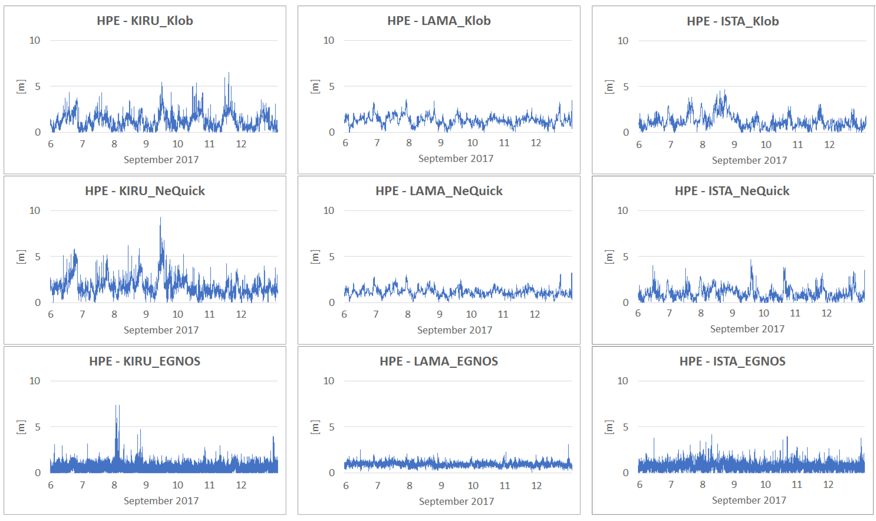
The results of the horizontal position error (HPE) for the analysed stations and ionosphere models are presented in
Figure 6 and
Table 2 on the left. The HPE is the difference between the reference (true) values of the stations’ coordinates and the coordinates calculated with the examined ionosphere models. The drawings clearly show that the largest fluctuations in horizontal positioning accuracy occurred at the northernmost station: KIRU. This seems to be mainly related with the localisation of KIRU site at high latitudes, which implicates two possible problems. First of all, there is no doubt that the positioning accuracy for such stations is affected by the much worse geometry of GNSS satellites and consequently higher values of DOP (Dilution of Precision) indices. This issue was analysed in detail by Wang [
48], which confirmed the significance of this factor. The second reason of the lower accuracy is a highly variable ionosphere. As is well recognised, the high-latitude scintillations, which occur also for quiet periods, may cause the GNSS signals’ loss of lock and consequently affect the accuracy and integrity of navigation performance.
Analysing the mean errors obtained for all the examined modes at the individual stations, the differences range from 0.57 to 1.78 m; surprisingly, the extreme values were observed at the KIRU station. The EGNOS ionosphere model was definitely the best and allowed achieving an accuracy that was almost two times better than the other options analysed. For the EGNOS model, the mean errors ranged from 0.57 m (KIRU) to 0.96 m (LAMA). For the other modes, mean errors of 1.01 m (ISTA—NeQuick) to 1.78 m (KIRU—NeQuick) were obtained. For the NeQuick model, the largest differences in accuracy related to the latitude of the stations were observed, ranging from 1.01 to 1.78 m; for the Klob model, these differences were not so significant and ranged from 1.23 to 1.33 m. The smallest impact of station location on the mean positioning error was obtained for the option without the ionosphere model (off), and it stretched from 1.39 to 1.45 m. The largest positioning errors were achieved on 8–9 September, during and the day after the climax of the storm, which is clearly visible at the KIRU and ISTA stations in the off, Klob, and NeQuick solutions. Considering the EGNOS model, it is hard to see differences due to time of day or ionospheric storm. At the LAMA station, in the off, Klob, NeQuick, and EGNOS solutions, the time of day and the impact of the storm are hardly visible. The maximum error was achieved for the off solution at KIRU, which reached as high as 14.43 m, while the rest of the maximum errors for various options/stations did not exceed 10 meters, and usually, these were short periods not exceeding a few dozen seconds. Sudden short decreases in accuracy were also observed for the EGNOS model at the KIRU station on 8 September. The lower accuracy in this case correlates well with the enhanced values of the AE-index (
Figure 3) corresponding to the main phase of the geomagnetic storm. Taking into account the southwardly oriented Interplanetary Magnetic Field (IMF) for these periods, one can assume that this effect is related with the extreme ionospheric variability at the auroral zone [
49]. It should be noted that although during these events the EGNOS model showed significant decreases in accuracy, the horizontal position errors did not exceed the limit values for APV-1 operations. However, it should be emphasised that EGNOS system users are informed about the decrease in EGNOS positioning quality within a maximum of 6 s, and the maximum error for the KIRU station did not exceed 7.36 m. To sum up, it can be concluded that the EGNOS model against the other three solutions (off, Klob, NeQuick) is clearly the best considering the accuracy of horizontal positioning reaching an average value for the stations considered of about 0.75 m. The differences between off, Klob, and NeQuick are not significantly distinct from each other, and the average mean error for these solutions reached a value of 1.34 m.
The results of vertical position error (VPE) are graphically shown in
Figure 7, and the numerical values are summarised in
Table 2 on the right. Similar to horizontal positioning, the largest fluctuations in accuracy were obtained for the KIRU station. This is especially visible for the off solution, which achieves clearly worse accuracy in the first four analysed days. Interestingly, the positioning in the last three days of the examined period was clearly worse for the Klob model. In the off solution, diagrams clearly show daily cycles of vertical positioning accuracy, while for solutions using ionosphere models, this phenomenon is almost imperceptible. Clearly, the worst results were obtained for the off solution, where the average error values ranged from 4.36 m (KIRU) to 3.02 (ISTA), reaching an average value for the three stations of 3.47 m. Results that were twice as good were obtained for solutions with the Klob and NeQuick models; for these models, the average error reached 1.50 m, and the NeQiuck solution turned out to be slightly better than that of Klob. Similarly to the horizontal results, the vertical positioning accuracy for the EGNOS model proved to be the best, achieving an excellent average value of 0.93 m. Looking at the results for the EGNOS model graphically, it seems that the LAMA station came out the best, but when analysing the numerical results, it turns out that the average error for the LAMA station was the biggest. At the LAMA station, unlike KIRU and ISTA, no sharp jumps in accuracy were observed, and the maximum error reached only 5.75 m. At the KIRU and ISTA stations, the maximum errors for the EGNOS model reached the values of 15.63 and 8.40 m, respectively; at these stations, there was a clear decrease in accuracy on 8 September. These high values of errors for the EGNOS model occurred during the climactic periods of the geomagnetic storm and coincide exactly with the peak values of the AE-index. Nevertheless, it should be emphasised that during these events, the vertical position errors did not exceed the limit values for APV-1 operations. The largest maximum errors were observed at the KIRU station and they amounted to 23.41, 11.99, 9.72, and 15.63 m for the off, Klob, NeQuck, and EGNOS modes respectively. In summary, it can be concluded that the EGNOS model against the other three solutions (off, Klob, NeQuick) is definitely the best considering the accuracy of vertical positioning, reaching an unprecedented average value of 0.93 m. The differences between the solutions using the Klob and NeQuick models are similar (approximately 1.50 m), but they were clearly worse than the EGNOS model. Definitely the poorest results were achieved for the off solution, in which the average error of 3.47 m was 2–3 times worse than the other results.
5. Conclusions
The article presents the results of GPS/EGNOS positioning using different ionosphere models at three IGS stations located at different latitudes during a strong ionospheric storm in September 2017. Four different positioning versions—without any ionosphere model (off), with Klobuchar model (Klob), NeQuick G model (NeQuick) and EGNOS model (EGNOS)—were analysed in the study. Although there was a strong magnetic storm during the period under review, culminating on 8 September 2017, the obtained accuracy seems to meet successfully the GPS SPS standards of 9 m for horizontal positioning and 15 m for vertical positioning with 95% probability. During the test, there were some moments when the errors reached higher values (for off solution), but they lasted for very few epochs. One of the reasons for obtaining such high accuracy is the use of the EGNOS clock and ephemeris corrections in all the examined solutions. The second reason is undoubtedly the fact that despite this storm being categorised as a G4 level storm in a five-level scale used by the NOAA (National Oceanic and Atmospheric Administration) and the Kp-index reaching 8+, the VTEC content over the analysed stations was not extremely high, reaching maximum values from 15 (KIRU) to 26 (ISTA). It is estimated that a higher value of VTEC could lead to more significant positioning errors.
As expected, the option with the EGNOS model came out the best, which for horizontal positioning was on average almost two times better than the other solutions. For vertical positioning, the EGNOS model proved to be two times better for the Klob and NeQuick models, while for off solution, it was more than three times better. The differences between Klob and NeQuick are not significantly distinct from each other; this was mainly caused by the similar (rare) update rate of these models. The rare update rate of these models does not take into account rapid ionosphere changes, which often happen during geomagnetic storms. It should be emphasised that the EGNOS model did not work as it was expected during the culmination of the storm at the beginning of 8 September. In this period, the EGNOS ionospheric model presented very large errors both in the horizontal and vertical directions. This anomaly was not observed for other examined models. This fact was caused by the very high magnetic activity produced by enhanced ionospheric currents flowing below and within the auroral oval (
Figure 3). This caused the instability of the EGNOS ionospheric model in the high latitude area and proves that further research is needed to improve the SBAS solutions to exclude such dangerous anomalies of operation. Nevertheless, the obtained results prove that the EGNOS ionospheric model meets the aviation positioning accuracy criteria for the APV-1 approach during the studied geomagnetic storm.
The graphical representation of the errors on charts suggests that the most stable GPS performance is at station located in mid-latitude: LAMA. The impact of auroral scintillations can be observed at northernmost station, KIRU, while at the southernmost station, ISTA, the influence of high solar flux that occurs at and near the equatorial crest level can be noticed. Nevertheless, the numerical results show that the latitude of the station does not have a severe impact on the overall accuracy of horizontal positioning; the average error values for four ionospheric variants range from 1.10 m (ISTA) to 1.26 m (LAMA). Much greater dependence of positioning accuracy due to latitude was recorded for vertical accuracy, whose average values for four ionospheric variants reached the values of 1.58 (ISTA), 1.72 m (LAMA), and 2.28 m (KIRU).
In the future research, it is planned to compare the performance of different ionospheric models during two periods (one with storm and other without any storms) with similar VTEC values, as this will allow extending the achieved results into more general cases.


