Investigation of Spatial Chirp Induced by Misalignments in a Parallel Grating Pair Pulse Stretcher

Abstract

Spatial chirp induced by the misaligned gratings and mirrors in a parallel grating pair pulse stretcher can significantly affect the performance of the output pulses. Firstly, a detailed analysis about the spatial chirp of the stretched pulses caused by the misalignments has been carried out using the ray tracing simulation method. According to the simulation results, an adjustment procedure has been summarized to accurately calibrate these misalignments. The proposed method has been successfully applied in a home-made chirped pulse stretcher. By measuring the output pulse with an imaging spectrometer, the results show the stretched pulse has a good linear temporal chirp and little spatial chirp, which demonstrates the good adjustment of the stretcher.

1. Introduction

A linear chirped pulse, of which the spectrum can be linearly mapped into the time domain, is often adopted as the probe pulse in the ultrafast dynamic measurements, such as the shock wave experiments [1,2], the dynamic metrology of plasmas or ionization [3,4], the single shot terahertz detection [5,6], the ultrafast transient absorption experiments [7,8], and the dynamic ellipsometry metrology of materials under extreme conditions [9]. In the above experiments, a pulse stretcher is needed to generate a linearly chirped pulse with a certain pulse width, in which chirp characteristics determine the practical measurement accuracy. Therefore, the accurate adjustment of the stretch system is of great importance.

In a chirped pulse stretcher system, gratings, prisms, or optical fibers are often employed as the chromatic dispersion elements [10,11,12,13]. Compared to the grating-based stretcher, a prism pair has smaller dispersion, and it is hard to obtain a long-duration chirped pulse. A long fiber possesses a high nonlinear dispersion and is limited only for relatively low pulse energy. Hence, the parallel grating pair pulse stretcher is more suitable to create a linear chirped pulse, in which pulse width can be easily adjusted by only changing the distance between the gratings. Since the misalignments of the gratings and mirrors in the stretcher (or compressor) can not only cause dispersion in the time domain (temporal chirp) [14,15] but also cause dispersion in the space domain (spatial chirp) [16,17,18,19,20], accurate adjustment of the stretcher is necessary to achieve an ideal linearly chirped pulse. Spatial chirp induced by the specific misalignment of the parallel grating pair has been theoretically analyzed, and several adjustment methods have been proposed [21,22,23]. However, it is difficult to evaluate the overall effects when two or more misalignments exist simultaneously, especially when taking the mirror adjustment errors into consideration. By utilizing extremely accurately manufactured roof mirrors or corner cubes, single-grating based stretchers or compressors have been proposed, which are more compact and show significant simplification in their adjustment [24,25]. In practice, limited by the element size and the great difficulty in manufacturing, the roof mirrors and corner cubes usually consist of two or three separate mirrors, leading the single grating structure to still possess the similar adjustment errors with the dual-grating structure. Therefore, it is highly desirable to investigate the criteria to describe the spatial chirp when several misalignments exist and summarize a feasible procedure for the misalignment calibration.

In this paper, a single grating pulse stretcher based on the dispersion theory of parallel grating pair has been built, which is designed for the shock compression experiment. By constructing a virtual stretch system in the Zemax software, the spatial chirp of the stretched pulse induced by different possible misalignments has been analyzed. Since the simulation results show little coupling effects among different misalignments, the spatial chirp induced by specific misalignment can be calibrated individually, and the overall effect is possible to be evaluated using superposition. According to the sensitivity analysis of the spatial chirp to different misalignments, we summarized the adjustment procedure. By applying the proposed procedure on the adjustment of our home-made pulse stretcher, the spatial chirp has been reduced to an ignorable level, demonstrating the good adjustment of our stretcher. The temporal chirp of the stretched pulse is also measured with the spectral interferometer [26]. Results show the output pulses have good linearity between wavelength and time, and its pulse width is well consistent with the designed value.

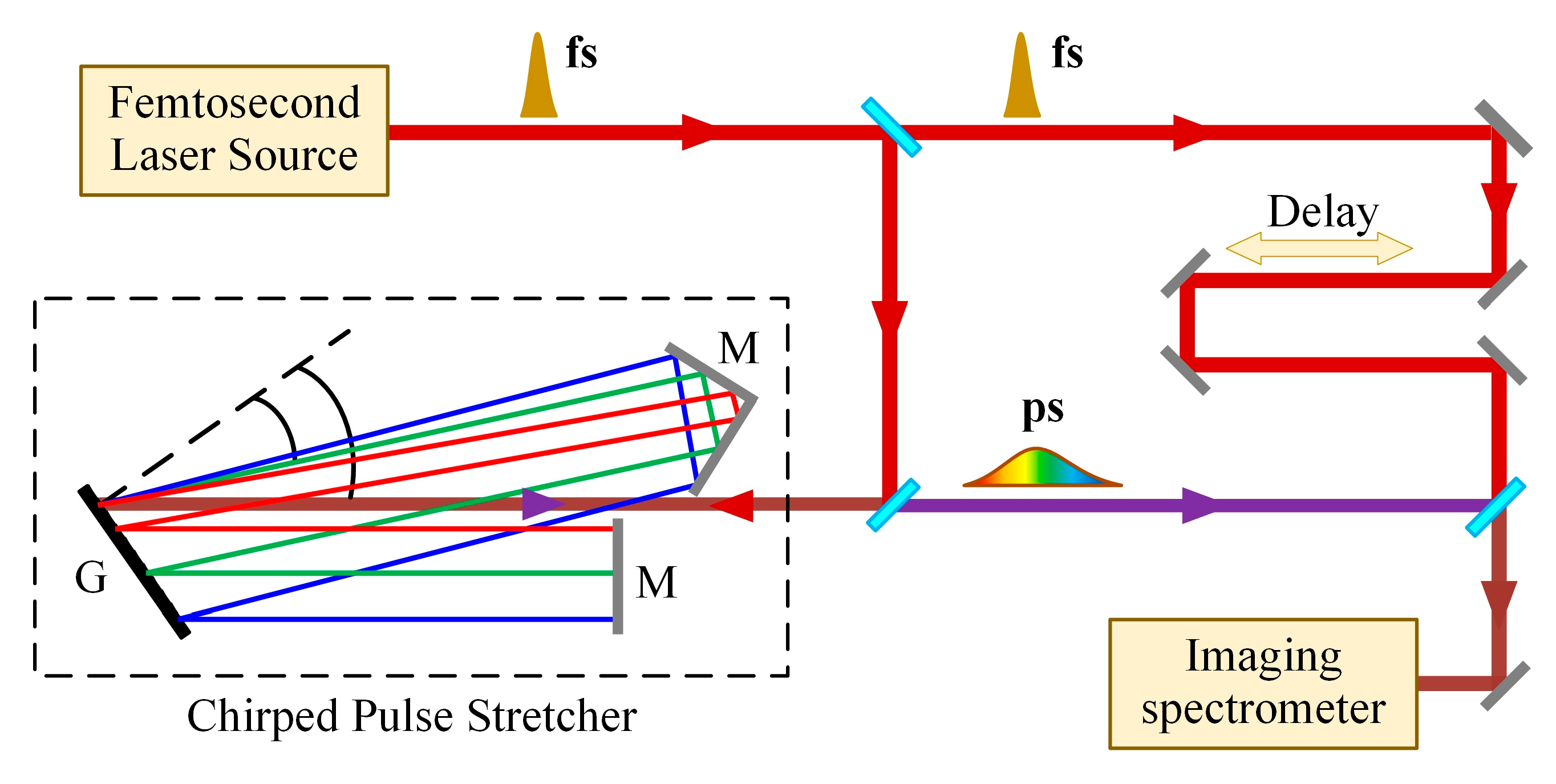
2. Design of Chirped Pulse Stretcher

To design a satisfactory pulse stretcher, we should first review the dispersion theory of the parallel grating pair. Figure 1a is the typical structure of a parallel grating pair stretcher. When an fs pulse propagates through the stretcher, the optical path of BCD can be expressed as:

$$L=\mathrm{BC}+\mathrm{CD}=L_0\left(\frac{1}{\cos \beta }+\cos \alpha +\sin \alpha \cdot \tan \beta \right),$$

(1)

where L₀ is the vertical distance between the grating pair, a and β are the incident angle and diffraction angle of the incident pulse, respectively.

The grating diffraction equation is:

$$\sin \alpha +\sin \beta ={10}^{-6}md\lambda ,$$

(2)

where m is the diffraction order, d is the groove density (lines/mm), and λ is the wavelength (nm). Combining Equation (2) and (1) can be rewritten as follows (for m = 1):

$$L=L_0\left(\frac{1+\sin \alpha \left({10}^{-6}d\lambda -\sin \alpha \right)}{\sqrt{1-{\left({10}^{-6}d\lambda -\sin \alpha \right)}^2}}+\cos \alpha \right).$$

(3)

Then, the chromatic dispersion of the parallel grating pair can be expressed as the derivative of L against the wavelength λ:

$$\frac{\mathrm{d}L}{\mathrm{d}\lambda }=\frac{L_0{\left({10}^{-6}d\right)}^2\lambda }{{\left[1-{\left({10}^{-6}d\lambda -\sin \alpha \right)}^2\right]}^{3/2}}.$$

(4)

According to Equation (4), we can find the dispersion of the grating pair is proportional to L₀. For a certain a and d, we can adjust its dispersion by only change the vertical distance L₀ between the grating pair. Since the pulses will pass through the stretcher twice, the pulse width τ_c of the stretched pulse can be expressed as:

$${\tau }_c=\frac{2\mathrm{d}L}{c}\approx \frac{2\cdot L_0{\left({10}^{-6}d\right)}^2{\lambda }_0\cdot \Delta \lambda }{c\cdot {\left[1-{\left({10}^{-6}d{\lambda }_0-\sin \alpha \right)}^2\right]}^{3/2}},$$

(5)

where λ₀ is the center wavelength of the pulse, and Δλ is the band width.

To achieve the dynamic parameters in a single shot in a shock compression experiment, a chirped pulse with good linearity and a relatively long duration is needed. Here, we choose the stretch principle of the parallel grating pair to build our own chirped pulse stretcher. The Ti:sapphire laser (Newport Corporation, SOL-ACE35F1K-HP) used in the experiment can output Gaussian limit pulses with about 7 mJ single pulse energy, which have a pulse width of about 35 fs and a band width of about 42 nm, while the center wavelength is about 800 nm. In our home-made stretcher, we use a horizontal roof mirror (HRM) to replace the second grating G2; thus, only one grating is needed, and the stretcher is more compact, as shown in Figure 1b. The vertical roof mirror (VRM) in the stretcher can make the input fs pulse and the output ps pulses propagate in two different heights so that the ps pulses can be directly outputted with a mirror instead of a beam splitter. A gold-coated blazed grating is employed in the stretcher, in which the groove density is 1200 lines/mm and its Littrow angle is 28.7°. To guarantee the diffraction efficiency of the gratings, the incident angle a is set as 35°. In the single grating structure, the incident pulses will hit the grating four times, and the optical path between two hits is equivalent to L₀, as shown in Figure 1a, which is set as 910mm. According to Equation (5), the pulse width of the stretched pulses can be calculated to be about 374.1 ps for the incident fs pulses with a band width of 42 nm and a center wavelength of 800 nm.

3. Spatial Chirp Induced by the Misalignments and its Adjustment

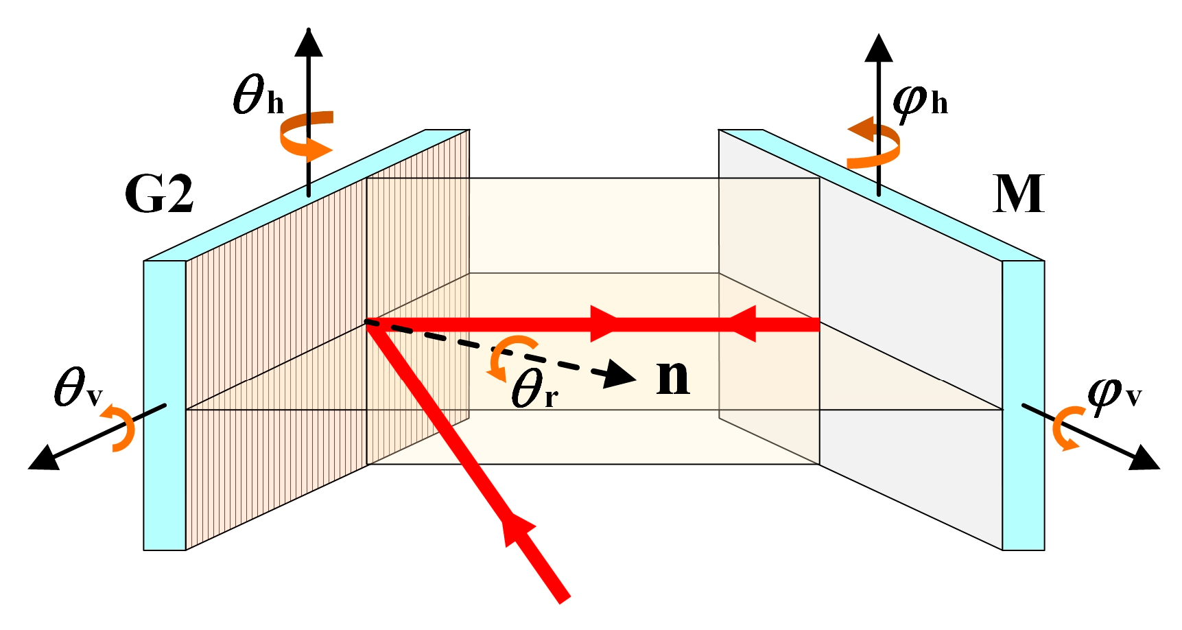
3.1. Misalignments of the Gratings and Mirrors in the Stretcher

Without losing generality, we only take the parallel grating pair structure shown in Figure 1a as an example to show the effects of misalignments in our simulation. Here, we define the direction parallel to the grating grooves as the vertical direction, while the direction perpendicular to the grooves as the horizontal direction. Thus, the adjustment errors of the grating pair and mirror consist of five components, such as the horizontal tilt of the gratings θ_h, the vertical tilt of the gratings θ_v, the unparallel groves between the two gratings θ_r, the horizontal tilt of the mirror φ_h, and the vertical tilt of the mirror φ_v. The schematic diagram of the five misalignments is shown in Figure 2. Since the first grating G1 has been selected as the baseline and is fixed, only the second grating G2 and the mirror M are shown in Figure 2 for brevity.

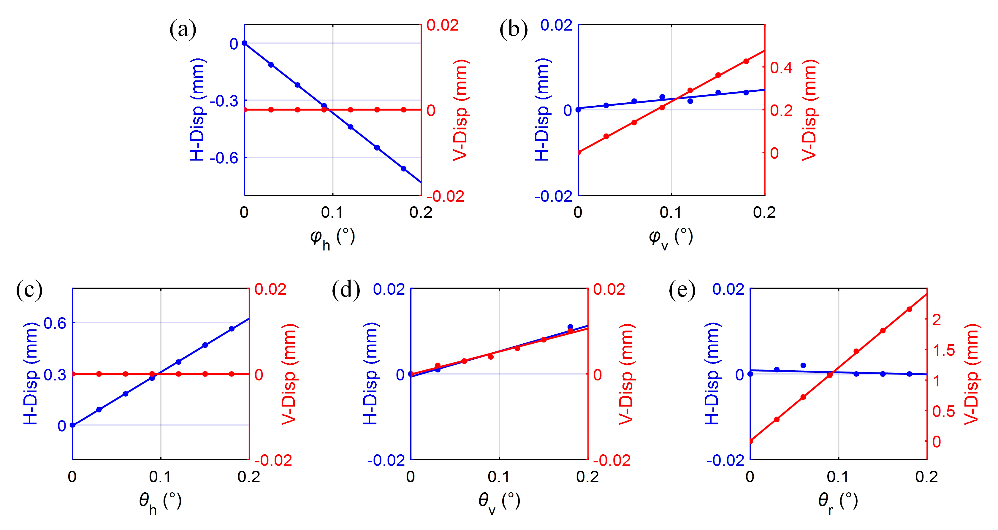
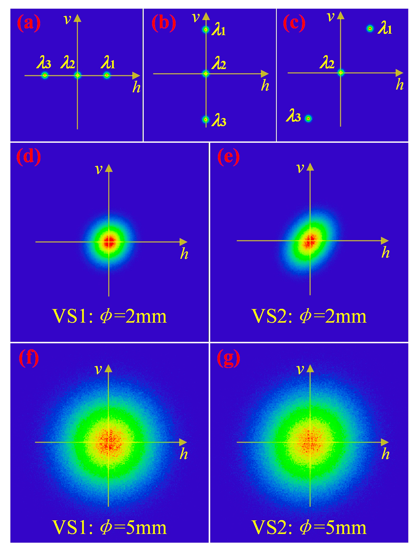
3.2. Spatial Chirp Analysis with the Ray Tracing Simulation Method

The spatial chirp caused by each one of the above five misalignments can be theoretical calculated [16,17,19,21,23]. However, due to the complexity of the theoretical equations, the interactions among different misalignments are unknown and are difficult to be analyzed; thus, the overall effects cannot be evaluated when two or more misalignments exist simultaneously. In this work, we use the Zemax software and the ray tracing simulation method to analyze the spatial chirp of the stretched pulses more visually.

In the Zemax software, we constructed an ideal parallel grating pair stretcher model, in which parameters are set the same as the designed values in our home-made stretcher described in Section 2. To simulate the spatial chirp induced by different misalignments, we just need to intentionally set the corresponding grating or mirror at a deviation from their designed value. Then, we use the ray tracing method to simulate the off-axis deviations (OFD) and the line dispersion (LD) induced by the misalignments on a view screen that is far away (3000 mm) from the first grating G1. Three different wavelengths λ₁ = 775 nm, λ₂ = 800 nm, and λ₃ = 825 nm are selected to carry out the simulation, which covers the major wavelengths of our fs pulses. First, we investigated the spatial chirp characteristics when each one misalignment exists individually. Figure 3 is the line dispersion between λ₁ and λ₃ induced by each misalignment, from which we can conclude that θ_h and φ_h can only cause dispersion in the horizontal direction, θ_r and φ_v can cause mainly dispersion in vertical direction and negligible dispersion in the horizontal direction, while θ_v cause very small dispersion in both the horizontal direction and vertical direction. It also can be seen that all the dispersion induced by each misalignment is changed approximately linear against the alignment error. Except line dispersion, misalignments can also lead to off-axis deviation.

Table 1. The spatial characteristics of the stretched pulses caused by the misalignments when the view screen is 3.0 m away from the first grating G1 of the stretcher.

Misalignments		Off-Axis Deviation (mm) of λ2 (800 nm)		Line Dispersion (mm) Between λ1 (775 nm) and λ3 (825 nm)
		Horizontal Direction	Vertical Direction	Horizontal Direction	Vertical Direction
Grating	θh = −0.2°	64.07	0	−0.57	0
	θv = −0.1°	0	27.55	0	0
	θr = 0.1°	0	−15.20	0	1.17
Mirror	φh = −0.424°	−64.28	0	1.56	0
	φv = −0.078°	0	−12.34	0	0.18
The five misalignments exist simultaneously		−0.05	−0.02	0.94	1.35

lists the full simulation results with one set of misalignments, from which we can conclude that θ_h and φ_h can cause the off-axis deviation in the horizontal direction, while θ_v, θ_r, and φ_v can only cause the off-axis deviation in the vertical direction. It can also be read from Table 1 that φ_h contributes the most to the line dispersion in the horizontal direction, while θ_r contributes the most to the line dispersion in the vertical direction. When the five misalignments exist simultaneously, the overall off-axis deviation and the line dispersion approximately equal to the linear superposition of the effects due to these misalignments when they exist individually. Simulation with several sets of misalignments have been carried out, and each set of data can achieve the same conclusions as above, indicating little coupling effects exist among different misalignments.

The values of θ_h, θ_v, and θ_r in Table 1 are set arbitrarily. In this situation, the off-axis deviation and the line dispersion will exist simultaneously. Then, the values of the rest two misalignments φ_h and φ_v are set intentionally to achieve the opposite off-axis deviations, so that their effects can counteract the effects due to the other three misalignments and the overall off-axis deviation becomes zero. This simulation configuration is rational because making the input pulses and the output pulses coaxial are the basic steps in the practical adjustment of the stretcher. Figure 4 schematically shows the spatial chirp induced by different misalignments, in which the simulation parameters are identical to those in Table 1. It can be observed that when the off-axis deviation is zero, their line dispersions still exist, resulting in an evident spatial chirp of the output pulses. Figure 4d,e shows the spot profiles of a stretched Gaussian pulse with a diameter of 2 mm when the view screens are 0.5 and 3.0 m away from the first grating G1, respectively. Since the spatial chirp is mainly from the angular dispersion, which cannot be directly observed, we used a view screen in the far field (3.0 m) to observe the line dispersion of the stretched pulses, which is clearer compared to the screen in the near field (0.5 m), as shown in Figure 4d,e. The spatial chirp can lead to an elliptical profile of the pulse spot, in which the direction can be used to distinguish the spatial chirp type. However, for the pulses with a relatively large diameter, the spatial chirp cannot be distinguished easily by the naked eye, as shown in Figure 4f,g, which is the same as Figure 4d,e, except the pulse diameter is 5 mm.

3.3. Adjustments Method to Calibrate the Misalignments

Since no significant coupling effects on the spatial chirp among different misalignments have been observed, the calibration of different misalignments can be carried out individually. According to the sensitivity of the spatial chirp to each misalignment, we have concluded a set of adjustment procedures, as described in Figure 5. The adjustment procedure can be roughly divided into two steps, the coarse adjustment and the fine adjustment. After assembling each element of the stretcher in their appropriate positions as designed, the first step is making sure the incident beams are in the horizontal direction before being projected on grating G1 in the coarse adjustment. Then, we need to adjust grating G2 and mirror M to make the output beam coaxial with the input beam. At this moment, the off-axis deviation of the output pulses can be regarded as zero in both the horizontal and vertical directions. The fine adjustment consists of two sub-steps. The first sub-step is adjusting the vertical chirp of the output pulse. Since the vertical tilt angle φ_v of M can be well adjusted individually, and it contributes little to the vertical chirp compared to θ_r according to Table 1, the vertical chirp can be regarded as being induced by the unparallel grooves of the grating pair only. Thus, we can just adjust θ_r to make the vertical chirp zero. Then, adjust the vertical tilt θ_v of G2 to make the off-axis deviation zero again. The second sub-step of the fine adjustment is adjusting the horizontal chirp. Since the horizontal tilt φ_h of M contributes to the horizontal chirp much more than the horizontal tilt θ_h of G2 does when the off-axis deviation is zero, we could adjust φ_h first to zero the horizontal chirp, and then adjust θ_h to make the off-axis deviation zero again. Repeat the above adjustments of φ_h and θ_h until both the spatial chirp and the off-axis deviation are zeros. Then, the off-axis deviation and the spatial chirp are zeros in both the vertical and horizontal directions, and the stretcher can be regarded as being well adjusted. Since the spatial chirp for the beam with a large diameter is difficult to be distinguished by the naked eye, an imaging spectrometer can be used for more precise real-time detection in the fine adjustment phase, which will be shown in Section 4.1.

For our home-made single grating stretcher shown in Figure 1b, each of the two roof mirrors consists of two plane mirrors. The non-perpendicularity between the two mirrors in HRM and VRM can be equivalent to the horizontal tilt of G2 and the vertical tilt of M in Figure 1a, respectively. The vertical tilt of HRM can be equivalent to the vertical tilt of G2 in Figure 1a, while the horizontal tilt of VRM can be equivalent to the horizontal tilt of M in Figure 1a. The grating rotation error for the two structures in Figure 1 are the same. Therefore, our single-grating structure has the same misalignments with the dual-grating structure, and the above adjustment procedure is still feasible.

4. Experimental results

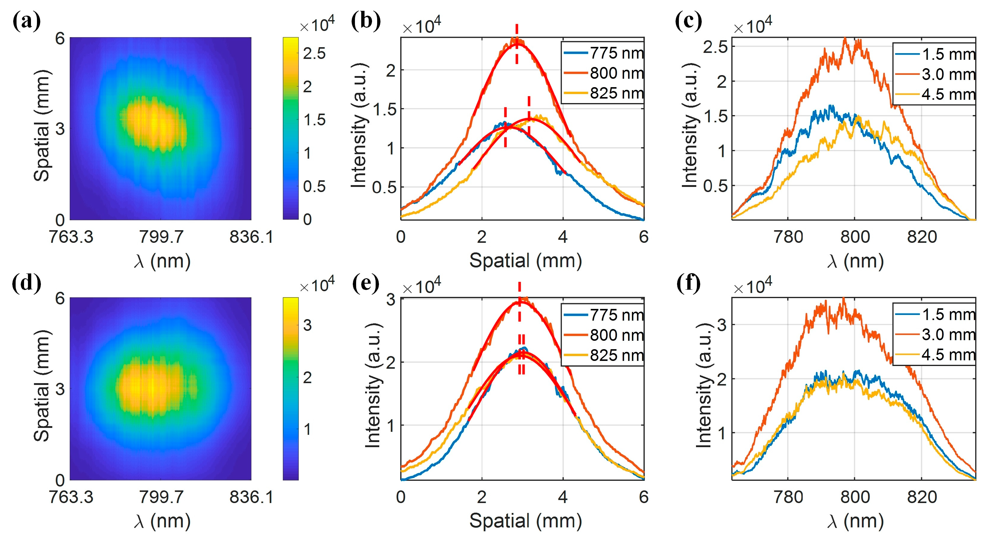
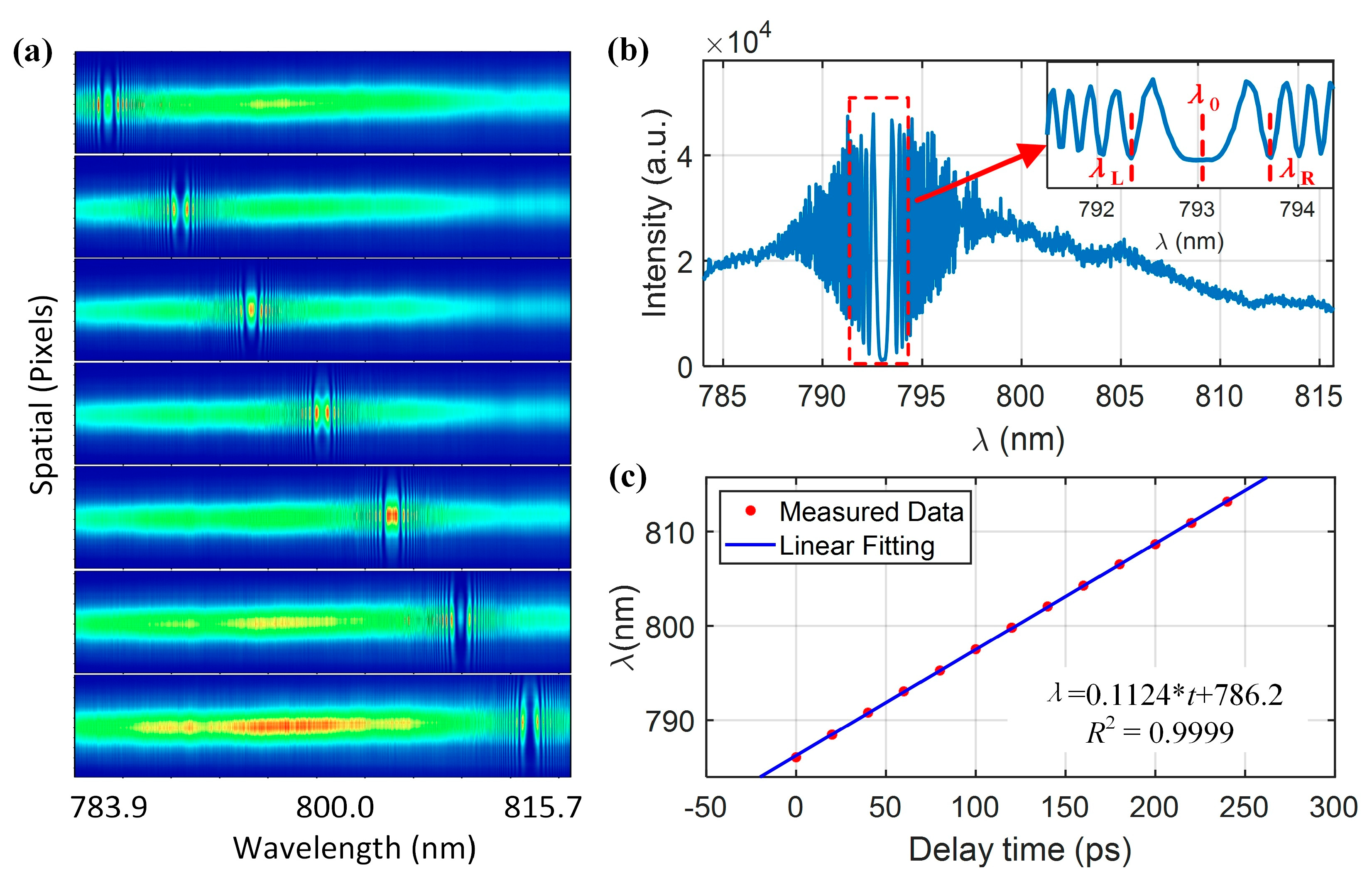
4.1. Spatial Chirp Measurement of the Stretched Pulse

For pulses with a large diameter, their spatial chirp may not be distinguished easily by the naked eye according to the spot profiles, as shown in Figure 4f,g. The initial diameter of the fs pulses output from our laser source is about 11 mm. After being stretched by the stretcher, we have changed its diameter to be about 5.5 mm with a 1/2 beam shrinker, which is still too large to observe its spatial chirp. Here, we use an imaging spectrometer (Horiba, iHR550) to detect the spatial chirp of the output pulses in real-time. The CCD detector (Horiba, Syncer-1024x256) attached to the imaging spectrometer can achieve the spectrum corresponding to a line of the light spot in the vertical direction. Figure 6a,d shows the spatial-spectrum of a stretched pulse with an evident vertical chirp and a pulse with little vertical chirp, respectively, both of which are obtained in one single pulse. According to Figure 6b,c, we can find that, for a pulse with a large vertical chirp, both the spatial profiles corresponding to different wavelengths and the spectrum profiles corresponding to different positions have an obvious shift. However, for a well-adjusted stretcher with little vertical chirp, both the spatial profiles and the spectrum profiles have a good overlap, as shown in Figure 6e,f. Therefore, we can use the above phenomenon to evaluate the vertical chirp of the pulses. In Figure 6c,f, we can find that the spectrum band width for the spatially chirped pulse is narrower than the unchirped pulse. This is reasonable because the spectrum for the spatially chirped pulse disperses in spatial, and only part of the spectrum enters into the slit of the spectrometer. Therefore, a narrower spectrum band width can also be regarded as evidence for the existence of spatial chirp. However, it is not convenient to evaluate the FWHM of spectrums because the spectrum profile in our experiment is not an ideal Gaussian profile. Thus, we prefer to use the spatial profile to analyze the spatial chirp here, which possesses a relative ideal Gaussian profile and is easy to identify its spatial center. To detect the horizontal chirp of a pulse, we just need to move the slit of the imaging spectrometer in the horizontal direction and observe whether there is a shift among their spectrum profiles, which are similar to those shown in Figure 6c,f.

Although the spatial chirp induced by each misalignment obeys “linear superposition”, we do not know their individual contribution to the overall effect, thus cannot give an accurate evaluation for each misalignment. Furthermore, misalignments cannot only cause spatial dispersion but also high order temporal dispersion [14,19]. When the grating pair structure acts as a pulse compressor, one can measure the spatial dispersion and the pulse duration simultaneously to obtain a more precise alignment procedure [22]. For our pulse stretcher, only the second order temporal dispersion (linear temporal chirp) is concerned, and the spatial chirp measurement is sufficient to achieve a satisfied adjustment accuracy.

4.2. Temporal Chirp Measurement of the Stretched Pulse

Since the incident angle of the pulses on the first grating and the vertical distance between the grating pair may deviate to their designed values, which will only affect the temporal chirp but not affect the spatial chirp of the stretched pulse, the temporal chirp offset to the designed value may still exist, even for a spatial chirp well-adjusted stretcher. In order to examine the performance of the stretcher, we have measured the actual temporal chirp of the stretched pulse with the time-delayed spectral interferometer. By making the stretched ps chirped pulse interfere with the unstretched fs pulse in the spectral domain, we can get the point-in-time corresponding to the wavelength in the center of the interference fringe. When setting the fs pulse with different delay times, the time corresponding to each wavelength of the chirped pulse can be obtained. Performing a linear fitting on the measured data, the linear chirp coefficient can be extracted. More theory and details about the method can be found in [26].

Figure 7 is the optical path employed in the temporal chirp measurement experiment. First, adjust the delayer at a proper position at which the time delay Δt between the fs beam and the ps beam is assumed to be zero. The first interferogram at Δt = 0 ps obtained in one single pulse is the top one in Figure 8a. Then, move the delayer to make the time delay Δt to be 20 ps between two adjacent measurements, and we can achieve more interferograms, as shown in Figure 8a, in which the spatial dimension has been compressed to show more interference patterns. Figure 8b is the interference fringe corresponding to a line of pixels in an interferogram. According to the theory, the spectrum λ₀ corresponding to the center of the widest fringe is the very point we need. First, we can find out the left fringe center λ_L and the right fringe center λ_R of λ₀, which are easier to be identified due to their narrower width, as shown in the partial enlarged drawing in Figure 8b. Then, λ₀ can be calculated by the equation λ₀ = (λ_L + λ_R) ÷ 2. With this method, we can find out all the points for interferograms with different time delays. Figure 8c is the spectrum against the time of the stretched chirped pulse. Performing a linear fitting on the measurement data, we have obtained the linear relationship between the wavelength and time, which can be expressed as λ = 0.1124 × t + 786.2. For the pulses with a band width of 42 nm, its corresponding stretched pulse width is about 373.7 ps, which is very close to its designed value 374.1 ps given in Section 2.

5. Conclusions

In this work, we analyzed the spatial chirp induced by the misalignments in the parallel grating pair pulse stretcher using the ray tracing simulation method. According to the simulation results, a simple adjustment method has been summarized that can accurately calibrate the misalignments. Measured with an imaging spectrometer, the stretched pulses of our home-made pulse stretcher show little spatial chirp, and its temporal chirp is well consistent with the designed value, indicating the stretcher we built has been well adjusted. The conclusions about the spatial chirp caused by the misalignments and the adjustment skills are also suitable for the cases when the parallel grating pair is adopted as a pulse compressor.

References

1. Geindre, J.P.; Audebert, P.; Rebibo, S.; Gauthier, J.C. Single-shot spectral interferometry with chirped pulses. Opt. Lett. 2001, 26, 1612–1614. [Google Scholar] [CrossRef]
2. McGrane, S.D.; Moore, D.S.; Funk, D.J.; Rabie, R.L. Spectrally modified chirped pulse generation of sustained shock waves. Appl. Phys. Lett. 2002, 80, 3919–3921. [Google Scholar] [CrossRef]
3. Chien, C.Y.; Fontaine, B.L.; Desparois, A.; Jiang, Z.; Johnston, T.W.; Kieffer, J.C.; Pepin, H.; Vidal, F. Single-shot chirped-pulse spectral interferometry used to measure the femtosecond ionization dynamics of air. Opt. Lett. 2000, 25, 578–580. [Google Scholar] [CrossRef] [PubMed]
4. Rebibo, S.; Geindre, J.P.; Audebert, P.; Grillon, G.; Chambaret, J.P.; Gauthier, J.C. Single-shot spectral interferometry of femtosecond laser-produced plasmas. Laser Part. Beams 2001, 19, 67–73. [Google Scholar] [CrossRef]
5. Zheng, S.; Lin, Q.; Cai, Y.; Zeng, X.; Li, Y.; Xu, S.; Li, J.; Fan, D. Improved common-path spectral interferometer for single-shot terahertz detection. Photonics Res. 2018, 6, 177. [Google Scholar] [CrossRef]
6. Yellampalle, B.; Kim, K.Y.; Rodriguez, G.; Glownia, J.H.; Taylor, A.J. Details of electro-optic terahertz detection with a chirped probe pulse. Opt. Express 2007, 15, 1376–1383. [Google Scholar] [CrossRef]
7. Shkrob, I.A.; Oulianov, D.A.; Crowell, R.A.; Pommeret, S. Frequency-domain “single-shot” ultrafast transient absorption spectroscopy using chirped laser pulses. J. Appl. Phys. 2004, 96, 25–33. [Google Scholar] [CrossRef] [Green Version]
8. Brown, K.E.; Bolme, C.A.; McGrane, S.D.; Moore, D.S. Ultrafast shock-induced chemistry in carbon disulfide probed with dynamic ellipsometry and transient absorption spectroscopy. J. Appl. Phys. 2015, 117, 085903. [Google Scholar] [CrossRef]
9. Shikne, R.; Yoneda, H. Ultrafast ellipsometric pump-probe diagnostic of liquid metal surface with chirped continuum probe pulses. Opt. Express 2015, 23, 20933–20940. [Google Scholar] [CrossRef]
10. Treacy, E. Optical pulse compression with diffraction gratings. IEEE J. Quantum Electron. 1969, 5, 454–458. [Google Scholar] [CrossRef]
11. Martinez, O. 3000 times grating compressor with positive group velocity dispersion: Application to fiber compensation in 1.3-1.6 µm region. IEEE J. Quantum Electron. 1987, 23, 59–64. [Google Scholar]
12. Martinez, O.E.; Gordon, J.P.; Fork, R.L. Negative group-velocity dispersion using refraction. J. Opt. Soc. Am. A 1984, 1, 1003–1006. [Google Scholar]
13. Galvanauskas, A. Mode-scalable fiber-based chirped pulse amplification systems. IEEE. J. Sel. Top. Quantum Electron. 2001, 7, 504–517. [Google Scholar] [CrossRef]
14. Zhang, Z.; Yagi, T. Evaluation of dispersion in a misaligned grating pair pulse compressor. J. Appl. Phys. 1995, 77, 937–939. [Google Scholar] [CrossRef]
15. Zhang, Z.; Yagi, T.; Arisawa, T. Ray-tracing model for stretcher dispersion calculation. Appl. Opt. 1997, 36, 3393–3399. [Google Scholar] [CrossRef]
16. Zhang, Z.; Harayama, S.; Yagi, T.; Arisawa, T. Vertical chirp in grating pair stretcher and compressor. Appl. Phys. Lett. 1995, 67, 176–178. [Google Scholar] [CrossRef]
17. Liu, W.; Zhu, Q.; Feng, G.; Jiang, D.; Zuo, Y.; Wang, X.; Chen, J. Study of dispersions on grating-pair compressor in the case of unparallel grooves. Optik 2006, 117, 236–239. [Google Scholar]
18. Daiya, D.; Patidar, R.K.; Sharma, J.; Joshi, A.S.; Naik, P.A.; Gupta, P.D. Optical design and studies of a tiled single grating pulse compressor for enhanced parametric space and compensation of tiling errors. Opt. Commun. 2017, 389, 165–169. [Google Scholar] [CrossRef]
19. Chen, Y.; Wang, C.; Zhang, Z.; Yang, X.; Xu, Y.; Leng, Y.; Xu, Z. Investigation of spatio-temporal stretching in a duplex grating compressor. Opt. Express 2019, 27, 31667–31675. [Google Scholar] [CrossRef]
20. Gu, X.; Akturk, S.; Trebino, R. Spatial chirp in ultrafast optics. Opt. Commun. 2004, 242, 599–604. [Google Scholar] [CrossRef]
21. Osvay, K.; Ross, I.N. On a pulse compressor with gratings having arbitrary orientation. Opt. Commun. 1994, 105, 271–278. [Google Scholar] [CrossRef]
22. Osvay, K.; Kovacs, A.P.; Heiner, Z.; Kurdi, G.; Klebniczki, J.; Csatari, M. Angular dispersion and temporal change of femtosecond pulses from misaligned pulse compressors. IEEE. J. Sel. Top. Quantum Electron. 2004, 10, 213–220. [Google Scholar] [CrossRef]
23. Guardalben, M.J. Littrow angle method to remove alignment errors in grating pulse compressors. Appl. Opt. 2008, 47, 4959–4964. [Google Scholar] [CrossRef] [PubMed]
24. Lai, M.; Lai, S.T.; Swinger, C. Single-grating laser pulse stretcher and compressor. Appl. Opt. 1994, 33, 6985–6987. [Google Scholar] [CrossRef] [PubMed]
25. Chauhan, V.; Bowlan, P.; Cohen, J.; Trebino, R. Single-diffraction-grating and grism pulse compressors. J. Opt. Soc. Am. B 2010, 27, 619–624. [Google Scholar] [CrossRef]
26. Fan, W.; Zhu, B.; Wu, Y.; Qian, F.; Shui, M.; Du, S.; Zhang, B.; Wu, Y.; Xin, J.; Zhao, Z.; et al. Measurement of the chirp characteristics of linearly chirped pulses by a frequency domain interference method. Opt. Express 2013, 21, 13062–13067. [Google Scholar] [CrossRef]
Figure 1. (a) The typical structure of a parallel grating pair chirped pulse stretcher, (b) the optical structure of our home-made stretcher with a single grating. BS, beam splitter; G, grating; M, mirror; a, incident angle; β, diffraction angle; L0, the vertical distance between the grating pair, HRM, horizontal roof mirror; VRM, vertical roof mirror. The arrows and numbers in (b) denote the light propagation order.
Applsci 10 01584 g001
Figure 2. The schematic diagram of the five misalignments of the grating and mirror in the stretcher. G2, the second grating in grating pair stretcher; n, the normal direction of G2; θh, the tilt angle error of grating G2 in the horizontal direction; θv, the tilt angle error of grating G2 in the vertical direction; θr, the rotation angle error of grating G2 that can lead to unparallel grooves of the grating pair; φh, the tilt angle error of mirror M in the horizontal direction; φv, the tilt angle error of mirror M in the horizontal direction. The arrows denote the positive direction.
Applsci 10 01584 g002
Figure 3. The line dispersion between λ1 (775 nm) and λ3 (825 nm) induced by each individual misalignment. (a,b) The horizontal tilt error and the vertical tilt error of M; (c,e) the horizontal tilt error, the vertical tilt error, and the rotation error of G2. H-Disp: the line dispersion in the horizontal direction; V-Disp: the line dispersion in the vertical dispersion.
Applsci 10 01584 g003
Figure 4. The spatial chirp of the output pulses induced by the stretcher misalignments. (a) The horizontal dispersion when only θh and φh exist, (b) the vertical dispersion when only θv, θr, and φv exist, (c) the dispersion when the five misalignments exist simultaneously. The simulation parameters used in (a)–(c) are identical to those in Table 1. (d,e) are the spot profiles of a stretched Gaussian pulse with a diameter of 2 mm when the view screens are 0.5 and 3.0 m away from the first grating G1, respectively. (f,g) are the same as (d,e), except the diameter of the pulse is 5 mm. VS1 and VS2 denote the position of the view screen is 0.5 and 3.0 m away from the first grating, respectively. The dimensions of (a)–(c) are 2 × 2 mm, while the dimensions of (e)–(g) are 10 × 10 mm.
Applsci 10 01584 g004
Figure 5. The flow chart to accurately calibrate the misalignments of the stretcher.
Applsci 10 01584 g005
Figure 6. The vertical chirp of the stretched pulses measured with an imaging spectrometer. (a) The spectrum corresponding to a vertical line of the light spot with a large vertical chirp; (b) the spatial profiles corresponding to three different wavelengths in (a), in which the centers show an obvious shift in vertical direction; (c) the spectrum corresponding to three different positions in (a), in which profiles also have an obvious shift; (d,e) the spatial-spectrum of an output pulse when the stretcher is well adjusted, which show little shift both in the spatial profiles and spectrum profiles, indicating the pulse has little vertical chirp.
Applsci 10 01584 g006
Figure 7. The optical path employed in the temporal chirp experiment.
Applsci 10 01584 g007
Figure 8. The measurement result of the temporal chirp of the stretched pulse. (a) The spectral interferograms between the fs pulse and the stretched ps chirped pulse with different delay times. The interferograms have been compressed in the spatial dimension to list more interferograms. (b) The interference fringe corresponding to a line of pixels in an interferogram; (c) the measurement data and the linear fitting between the wavelength and the delay time.
Applsci 10 01584 g008