A New Approach to Identifying Crash Hotspot Intersections (CHIs) Using Spatial Weights Matrices

Abstract

In this paper we develop a new approach to directly detect crash hotspot intersections (CHIs) using two customized spatial weights matrices, which are the inverse network distance-band spatial weights matrix of intersections (INDSWMI) and the k-nearest distance-band spatial weights matrix between crash and intersection (KDSWMCI). This new approach has three major steps. The first step is to build the INDSWMI by forming the road network, extracting the intersections from road junctions, and constructing the INDSWMI with road network constraints. The second step is to build the KDSWMCI by obtaining the adjacency crashes for each intersection. The third step is to perform intersection hotspot analysis (IHA) by using the Getis–Ord Gi* statistic with the INDSWMI and KDSWMCI to identify CHIs and test the Intersection Prediction Accuracy Index (IPAI). This approach is validated by comparison of the IPAI obtained using open street map (OSM) roads and intersection-related crashes (2008–2017) from Spencer city, Iowa, USA. The findings of the comparison show that higher prediction accuracy is achieved by using the proposed approach in identifying CHIs.

1. Introduction

The nation’s transportation infrastructural systems are deteriorating [1] under adverse influences from multiple factors, such as corrosion [2,3], aging [4], impact [5,6], and vibration [7], and even with the recent advances in structural health monitoring [8,9,10] and intelligent transportation systems [11,12], traffic crashes still happen. The latest quick facts report from the National Highway Traffic Safety Administration indicates that there were 2,746,000 people injured in 6,452,000 police-reported crashes in 2017 in the USA [13]. As junctions of traffic flow and pedestrian flow, intersections with ancillary facilities have an important impact on the frequency of crashes. Intersection-related crashes, which account for a large portion of all crashes, need more research attention. For example, Iowa, USA, saw about 225,185 intersection-related crashes, about 40.41% of all crashes, from 2008 to 2018 [14]. Given the fact of the massive number of intersections, identifying crash hotspot intersections (CHIs) is an important but challenging task.

A review of previous studies shows that the Getis–Ord Gi*, well known in hotspot analysis, has been commonly used to detect crash hotspots [15]. Hotspot analysis examines the Getis–Ord Gi* statistic [16,17], a local indicator of spatial autocorrelation developed by Professor Arthur Getis and J. Keith Ord, for individual crashes based on a comparison with neighboring crashes to quantitatively describe crashes and hotspot areas where crashes are mainly concentrated. Ouni et al. [18] discussed the identification of hot zones and enhanced the capability to examine a given highway by determining dangerous segments. Khan et al. [19] used the Getis–Ord Gi* statistic to analyze weather-related crashes which occurred in adverse weather conditions. Prasannakumar et al. [20] assessed the spatial clustering of accidents and hotspots’ spatial densities using the Getis–Ord Gi* statistic. Erdogan et al. [21] compared traditional hotspot detection methods with spatial statistical methods, including the Getis–Ord Gi* statistic, in terms of their sensitivity to spatial characteristics of crash clusters. Kuo et al. [22] combined kernel density estimation and Getis–Ord Gi* maps to identify high-risk areas for traffic crash hotspots and crime events. Zahran et al. [23] presented a new method to evaluate the application of four different hotspot analysis methods, such as Getis–Ord Gi*, in ArcGIS 10.2 to identify and rank hotspots using historical data on a section of a road in Brunei Darussalam. Memisoglu [24] et al. used hotspot analysis (Getis–Ord Gi*) and the kernel density method to identify traffic accident hotspots for traffic safety.

The above studies focused on using the Getis–Ord Gi* statistic to identify crash hotspots. Unlike crash hotspot analysis, only a limited number of studies have been dedicated to analyzing the spatial relationships between intersections and traffic crashes. Mitra [25] indicated that unstructured effects were somewhat significant at the intersection level for cases of severe-injury crashes. Cheng et al. [26] presented a crash evolution characteristic analysis for identifying hotspots among Wujiang’s road intersections. Cinnamon et al. [27] examined the potential associations between violations made by pedestrians and motorists at intersections.

Furthermore, the results of hotspot analysis using the Getis–Ord Gi* statistic in the above research were determined using critical input spatial weights matrices (SWMs) [28,29]. The related theories of general SWMs, such as contiguity-based SWMs [30,31], distance-band SWMs [32,33], and k-nearest neighbor SWMs [34], have been widely discussed. However, the general SWMs, which are designed for plane space, cannot provide good support for hotspot analysis in road network space. Therefore, we should improve the construction algorithms and build customized SWMs based on the above general SWM to adapt the identification approach of CHIs. The above studies provide a foundation for this research. However, previous studies neglected some issues in using hotspot analysis. First, these studies mainly focused on the crashes essentially as a phenomenon related to roads or intersections, and could not directly identify CHIs. Second, often the Euclidean distance was used to calculate the weights, neglecting road network restrictions, which may affect the accuracy of the result of hotspot analysis.

To solve these issues, first, we take intersections instead of crashes as the research object, which can directly identify CHIs. Second, the inverse network distance-band spatial weights matrix of intersections (INDSWMI) and the k-nearest distance-band spatial weights matrix between crash and intersection (KDSWMCI) are developed and applied to hotspot analysis to improve the accuracy of the results of CHI identification. The main tasks of this study include (a) creating the INDSWMI with respect to road network restraints; (b) building the KDSWMCI based on the k-nearest neighbors and distance-bands by obtaining the adjacency crashes and the number of crashes at each intersection; (c) testing the Intersection Prediction Accuracy Index (IPAI) of the proposed approach and identifying the CHIs to help safety researchers develop safety strategies to reduce crashes.

The rest of the paper is organized as follows. Section 2 presents the methodology developed in this paper. Section 3 describes the original data, including the road network and traffic crashes of Spencer city, Iowa. Section 4 illustrates and discusses the results by applying the proposed methodology to Spencer city, Iowa. Finally, Section 5 concludes the paper and recommends future work.

2. Methodology

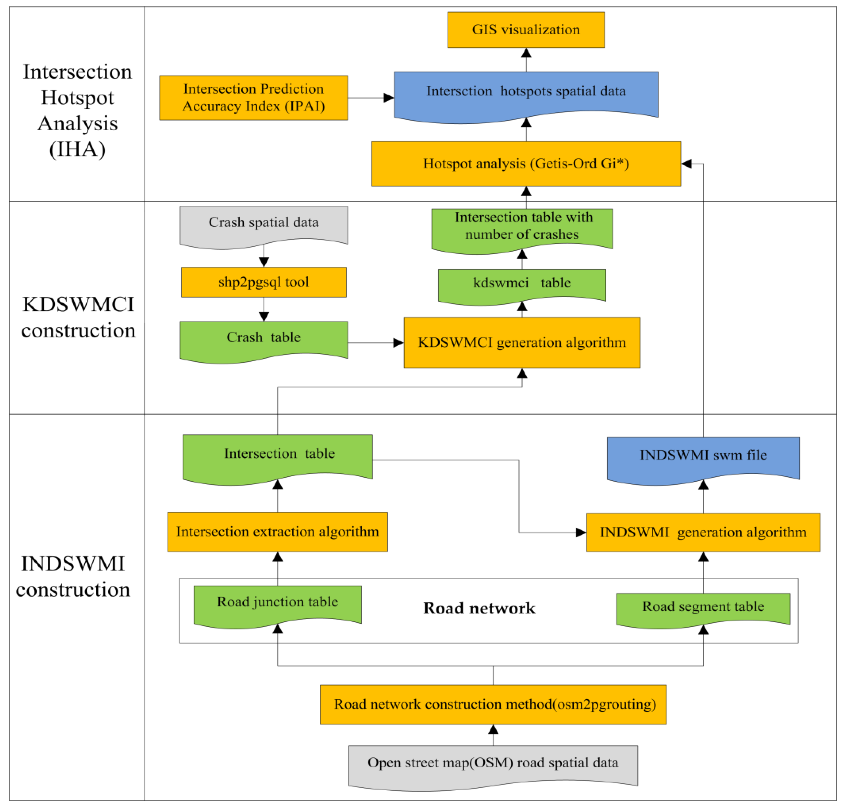
2.1. Process Map

This paper presents a three-step approach to directly identifying crash hotspot intersections (CHIs) by using (1) construction of the inverse network distance-band spatial weights matrix of intersection (INDSWMI), (2) construction of the k-nearest distance-band spatial weights matrix between crash and intersection (KDSWMCI), and (3) intersection hotspot analysis (IHA). The process map for the approach is shown in Figure 1.

(1) INDSWMI construction

The first step (INDSWMI construction) includes the following three substeps:

(a)

Road network construction. In this research, we apply osm2pgrouting [35], an open source software product, to build the road network including road junction and segment tables from the open street map (OSM) [36] road spatial dataset.

(b)

Intersection extraction. Note that a road junction that links with three or more road segments is considered an intersection, which is a junction of traffic flow and pedestrian flow [37,38] in this research. We developed an intersection extraction algorithm to extract intersections, such as T-intersection, Y-intersections, cross-intersections, and X-intersections [39], from the road junction table and create the intersection table. The intersection extraction algorithm can be described as the following structured query language (SQL) script:”create table public.intersection as select * from public.road_junction a where a.degree> 2”.

(c)

INDSWMI construction. We developed the INDSWMI generation algorithm to construct the INDSWMI, which can conceptualize the spatial relationships between intersections, with road network constraints based on the intersection table and road segment table. The INDSWMI is saved in the swm file format which is compatible with ArcGIS.

(2) KDSWMCI construction

The second step (KDSWMCI construction) is to conceptualize the crash–intersection spatial relationships. We developed the KDSWMCI generation algorithm to calculate the number of crashes and adjacency crashes of each intersection and save the crash–intersection spatial relationships in the KDSWMCI table.

(3) Intersection hotspot analysis

The third step, intersection hotspot analysis, is to identify CHIs using a statistical variable—Getis–Ord Gi*. The intersection hotspot analysis (IHA) generates the intersection hotspots shapefile using the standardized Getis–Ord Gi* of each intersection under randomization null hypothesis [40] computation. We can detect CHIs through geographic information system (GIS) visualization of the intersection hotspots shapefile. The Intersection Prediction Accuracy Index (IPAI) was calculated to quantitatively evaluate the prediction performance of IHA.

2.2. Data Types

There are three types of data in this approach: (1) the input data, (2) the intermediate data, and (3) the output data, as shown in

Table 1. An overview of data types.

Name	Type	File Format	Feature Type	Description
OSM Road	Input	osm	Line/Point/Region	Widely used open access geographic data
Crash	Input	shapefile	Point	The geographic data of crashes
Road junction	Intermediate	PostGreSQL Table	Point	The road junction spatial table generated by osm2pgrouting software
Road segment	Intermediate	PostGreSQL Table	Line	The road segment spatial table generated by osm2pgrouting software
Crash table	Intermediate	PostGreSQL Table	Point	The crash spatial table converted by shp2pgsql tool
Intersection	Intermediate	PostGreSQL Table	Point	The intersection spatial table with number of crashes extracted from road junction
KDSWMCI table	Intermediate	PostGreSQL Table	/	Stores the crash–intersection spatial relationships
INDSWMI file	Output	SWM	/	SWM format file with INDSWMI info from ArcGIS
Crash hotspot intersections	Output	Shapefile	Line	The result of intersection hotspot analysis

.

2.2.1. The Input Data

Two data sets are required as the inputs for this approach: the OSM road data and the crash shapefile. The OSM road data should contain the geometric info (a list of point coordinates) and the “highway” attribute. Note that “highway” in British English is used to indicate any type of road, such as motorway, primary, route, footway, and pedestrian, within OSM. In this research, we selected only the highways for cars, such as motorway, primary, secondary, tertiary, residential, and service, since we focused on traffic intersections. The crash shapefile should contain the geometric info (x-coordinate, y-coordinate) that is used to locate crashes on intersections. Crash-related factors [41,42], such as environment and driver, and crash attributes, such as crash type and date, are not necessary but are suggested.

2.2.2. The Intermediate Data

Intermediate files include a series of tables, such as crash, road junction, road segment, KDSWMCI, and intersection tables. The crash table was converted by using the shp2pgsql tool. The road junction and road segment tables, generated by osm2pgrouting software, contain the topological information and form of the road network. Note that the osm2pgrouting software cannot generate the intersection table. We developed an intersection extraction algorithm to build the intersection table with attributes such as the degree and type based on road network topological information.

In this research, we used PostGreSQL [43], a widely used open source database management system (DBMS), and PostGIS [44], an open source geospatial engine for PostgreSQL, to store and query spatial data of roads, intersections, and crashes. The geometry and attributes of the above tables were inherited from the input OSM road data and crash shapefile.

2.2.3. Output Results

The INDSWMI file and intersection hotspot shapefile are the output results. The INDSWMI file is constructed based on the network distance of intersections to conceptualize the intersection spatial relationships as a foundation for IHA. To improve the effectiveness of the approach, we used the binary swm file format, which is compatible with ArcGIS [45], to store INDSWMI data. Each row in a binary swm format file is formatted into four columns: OBJECTID (row index), GID (the ID of intersection i), NID (the ID of intersection j), and WEIGHT (the spatial weight between intersection GID and NID). The intersection hotspot shapefile, the result of the IHA (Getis–Ord Gi*), contains the hotspot intersections, coldspot intersections, and non-significant intersections. The hotspot intersections are the results that we should identify in this research.

2.3. Methods

2.3.1. The INDSWMI Generation Algorithm

A spatial weights matrix (SWM), the conceptualization of spatial relationships between features [46], is the key input parameter for hotspot analysis. The SWMs can be mainly divided into contiguity-based spatial weights matrices (CSWMs) and distance-band spatial weights matrices (DSWMs). The CSWM, which expresses the existence of a neighbor relation as a binary value, 1 or 0, is widely used in region-based hotspot analysis [47]. The DSWM, which expresses the spatial relationships as distance weights [48], is intrinsically most appropriate for point-based hotspot analysis. We adopted the DSWM to express the spatial relationships between intersections since intersections are a typical point feature.

The inverse network distance-band spatial weights matrix of intersections (INDSWMI) based on the DSWM is an N×N matrix. Generally, W_ij is defined using inverse Euclidean distance measurement. However, intersections are constrained by the road network, which has complex topological and geometric relationships [49]. The inverse network distance along the road is more appropriate for the measurement of W_ij of the INDSWMI, which is defined as

$$W_{ij}=\{\begin{array}{l}1/n{d}_{ij},n{d}_{ij}\le distanceband\\ 0,n{d}_{ij}>distanceband\end{array}$$

(1)

where the distance band is a cutoff distance that can be specified in accordance with the minimum number of neighbors of each intersection (the minimum number of neighbors is 1 in this research according to the suggestion of Getis and Aldstadt [29]); nd_ij is the network distance between intersections i and j. If nd_ij is less than or equal to the distance band, then W_ij = 1/nd_ij (reverse network distance); otherwise, W_ij = 0. nd_ij is expressed as

$$n{d}_{ij}={\displaystyle \sum _{k=1}^{n}length(r_k,r_k\in sp(I_i,I_j))}$$

(2)

where sp(I_i, I_j) is the shortest path set of intersections i and j, calculated by Dijkstra’s algorithm [50], and contains a series of road segments (r_k); nd_ij is the total length of road segments within sp(I_i, I_j).

Note that row standardization of W_ij is suggested to create proportional weights in cases where intersections have an unequal number of neighbor intersections [29]. The row-standardized form of W_{i j} for hotspot analysis is expressed as

$$W_{ij}=\{\begin{array}{c}\frac{1/n{d}_{ij}}{{\displaystyle \sum _{j=1}^{n}1/n{d}_{ij}}},\begin{array}{c}\\ \end{array}n{d}_{ij}\le distance\begin{array}{c}\\ \end{array}band\\ 0\begin{array}{c}\\ \end{array}\begin{array}{c}\\ \end{array}\begin{array}{c}\\ \end{array}\begin{array}{c}\\ \end{array}\begin{array}{c}\\ \end{array}\begin{array}{c}\\ \end{array},\begin{array}{c}\\ \end{array}n{d}_{ij}>distance\begin{array}{c}\\ \end{array}band\end{array}$$

(3)

Based on Equations (1) and (2), we used the qt framework [51], an open source cross-platform, to develop the INDSWMI generation algorithm with PostGreSQL/PostGIS. Figure 2 shows the definitions of the main data types: intersection, network distance of intersections (NDI), network distance matrix of intersections (NDMI), spatial weight of intersections (SWI), and INDSWMI.

Using the main data types, we developed a five-step algorithm with pseudocode shown in Figure 3 to generate the INDSWMI. The five steps are to (1) connect to the PostGreSQL/PostGIS database; (2) cache the intersection table in the PostGreSQL/PostGIS database to memory; (3) build the NDMI using the pgr_dijkstra fuction provided by the pgrouting extension for the PostGreSQL/PostGIS database; (4) generate the INDSWMI based on the NDMI restricted by the distance band; and (5) save the INDSWMI to the swm file format.

2.3.2. The KDSWMCI Generation Algorithm

To identify the crash hotspot intersections (CHIs), we should build the k-nearest distance-band spatial weights matrix between crash and intersection (KDSWMCI, k=1) based on CSWM by obtaining the adjacency crashes and the number of crashes at each intersection.

Generally, an SWM is an N×N matrix whose elements are spatial weights. In this research, we expanded the SWM to an M×N matrix, as shown in Equation (4), which can accommodate different numbers of intersections and crashes. There is one row for each intersection and one column for each crash.

$$KDSWMIC=\begin{array}{ccccc}& 1& 2& j& n\\ 1& {{\displaystyle w}}_{11}& {{\displaystyle w}}_{12}& {{\displaystyle w}}_{1j}& {{\displaystyle w}}_{1n}\\ 2& {{\displaystyle w}}_{21}& {{\displaystyle w}}_{22}& {{\displaystyle w}}_{2j}& {{\displaystyle w}}_{2n}\\ i& {{\displaystyle w}}_{i1}& {{\displaystyle w}}_{i1}& {{\displaystyle w}}_{ij}& {{\displaystyle w}}_{in}\\ m& {{\displaystyle w}}_{\mathrm{m}1}& {{\displaystyle w}}_{m2}& {{\displaystyle w}}_{mj}& {{\displaystyle w}}_{mn}\end{array}$$

(4)

Here, m is the number of crashes; n is the number of intersections; i is the unique identifier of a crash; j is the unique identifier of an intersection; and W_ij is the weight that quantifies the spatial relationship between crashes and intersections. If crash i occurs on intersection j, then W_ij = 1; otherwise, W_ij = 0. We can determine that a crash is on an intersection if the geometric relationships between the crash and intersection meet both of Conditions 1 and 2:

• Condition 1: The shortest distance between the crash and the intersection is less than or equal to the threshold distance.
• Condition 2: The intersection-related crash relates to one, and only one, intersection. That means that the k-nearest neighbor is the same as the 1st-nearest neighbor. Therefore, if crash i occurs on intersection j, then the shortest distance between crash i and intersection j should be the minimum distance in all datasets.

According to Conditions (1) and (2), the weight of the KDSWMCI is expressed as

$$W_{ij}=\{\begin{array}{c}1,\begin{array}{c}\\ \end{array}if\begin{array}{c}\\ \end{array}{d}_{ij}\le threshold\begin{array}{c}\\ \end{array}distance\begin{array}{c}\\ \end{array}and\begin{array}{c}\\ \end{array}{d}_{ij}\le \forall d_{ik}\\ 0\begin{array}{c}\\ \end{array},\begin{array}{c}\\ \end{array}else\end{array}$$

(5)

where d_ij is the Euclidean distance between crash i and intersection j; d_ik is the Euclidean distance between crash i and intersection k. A threshold distance of 28.5 m was selected by considering ten-lane intersections and Global Positioning System (GPS) positioning accuracy according to the following premises:

Premise 1

Crash GPS coordinates have a positioning error of approximately 10 m [52]. A crash is considered to occur on the intersection if its coordinates are within 10 m of the buffer of the intersection considering the positioning error.

Premise 2

As the Interstate Highway standards for the U.S. Interstate Highway System use a 12 foot (3.7 m) standard lane width, a crash occurring on the intersection can be determined if its coordinates are within (3.7 × n/2) m of the buffer of the intersection, where n is the number of lanes of the intersection.

We realized the KDSWMCI generation algorithm based on the qt framework with the PostGreSQL/PostGIS database. Figure 4 shows the definitions of the main data types: crash, spatial weight between crash and intersection (SWCI), and KDSWMCI. Note that the structure of intersections used in the algorithm is defined in Figure 2.

Based on the main data types, we developed a five-step algorithm with pseudocode shown in Figure 5 to generate the KDSWMCI: (1) connect to the PostGreSQL/PostGIS database; (2) cache the intersection and crash table in the PostGreSQL/PostGIS database to memory; (3) build the KDSWMCI using the st_within function and Euclidean distance measurement provided by the postgis extension for PostGreSQL to determine whether a crash is on an intersection according to Conditions 1 and 2; (4) save the crash–intersection spatial relationships to the KDSWMCI table in the PostGreSQL/PostGIS database; (5) compute the number of crashes for each intersection based on the KDSWMCI table.

2.3.3. Intersection Hotspot Analysis (Getis–Ord Gi*)

The Getis–Ord G, including Getis–Ord General G and Getis–Ord Gi^* [16], is one of the preferred measurement techniques for hotspot analysis [53]. The Getis–Ord General G is a single index that can detect the degree of autocorrelation to verify the spatial distribution pattern in the entire spatial extent. The Getis–Ord Gi^* is used as a local indicator [54] of spatial autocorrelation in IHA to identify CHIs. The Getis–Ord G_i^* was calculated for each intersection to reveal the degree of spatial autocorrelation and was used to analyze whether the same variable (<num_crash> in this research) has spatial autocorrelation. The Getis–Ord Gi^* is expressed as [16]

$${{\displaystyle G}}_i^{*}=\frac{{\displaystyle \sum _{j=1}^n{{\displaystyle w}}_{ij}{{\displaystyle x}}_j}}{{\displaystyle \sum _{j=1}^n{{\displaystyle x}}_j}}$$

(6)

where Gi^* is the statistic that expresses the spatial degree of spatial autocorrelation of intersection i with the number of crashes over all neighboring intersections; W_ij is the weight in the INDSWMI (discussed in Section 2.3.1) that quantifies the spatial relationship between intersection i and intersection j; x_j is the number of crashes at intersection j (discussed in Section 2.3.2 based on the KDSWMCI); and n is the total number of neighboring intersections.

According to the first law of geography, the number of crashes at an intersection, related to each other in geography, has a spatial distribution pattern that is either dispersed, random, or clustered [55]. The spatial distribution of the Gi^* statistic is random when randomness is also observed in the underlying distribution of the number of crashes at intersections. However, crashes have a clustered distribution pattern in reality. Therefore, in IHA, it is necessary to make assumptions about the spatial distribution of the number of crashes at intersections, which is the randomization null hypothesis. Testing of the randomization null hypothesis of spatial distribution can be performed based on the z-score (a standardized statistic) of the Gi^*, as shown in Equation (7) [56], along with the p-value (a probability value used to express the confidence level).

$$G_i^{*}ZScore=\frac{{\displaystyle \sum _{j=1}^n{w}_{ij}{x}_j-\overline{X}{\displaystyle \sum _{j=1}^n{w}_{ij}}}}{S\sqrt{\frac{[n{\displaystyle \sum _{j=1}^n{w}_{ij}{}^2-}{\left({\displaystyle \sum _{j=1}^n{w}_{ij}}\right)}^2]}{n-1}}}$$

(7)

Here, Gi^*ZScore is the standardized Gi^* value of intersection i. The Gi^*ZScores are measures of statistical significance which inform us whether or not to reject the randomization null hypothesis, intersection by intersection. In this study, p-values of ≤0.05 (95% confidence level) were used to indicate different levels of significant clusters, which were applied to each intersection. To be more specific, if an intersection’s p-value was >0.05 and its Gi^*ZScore was >1.96 [57], that intersection was considered a hotspot intersection at the 95% confidence level. W_ij is the weight in the INDSWMI, x_j is the number of crashes at intersection j calculated in the KDSWMCI, and $\overline{x}$ is the average number of crashes at all neighboring intersections. S is related to the measurement of sample variance and is defined as [56]

$$\overline{X}=\frac{{\displaystyle \sum _{j=1}^n{{\displaystyle x}}_j}}{\mathrm{n}}S=\sqrt{\frac{{\displaystyle \sum _{j=1}^n{x}_j{}^2}}{n}-{\left(\overline{X}\right)}^2}.$$

(8)

2.3.4. The Intersection Prediction Accuracy Index (IPAI)

Evaluation of hotspot analysis prediction performance is an important issue relating to the suitability of this proposed approach. The Prediction Accuracy Index (PAI) [58], firstly proposed by Chainey et al., is the ratio of the hit rate to the fraction of area covered [59]. The PAI has been widely applied to measure hotspot analysis results [17,59,60,61]. Previously, the Crash Prediction Accuracy Index (CPAI) was developed by using road length rather than area for evaluating traffic crash hotspot analysis performance [17,61]. Based on the previous studies, the Intersection Prediction Accuracy Index (IPAI) was developed in this research with road network restraints for evaluating IHA prediction performance as follows:

$$IPAI=\frac{{\displaystyle \sum _{j=1}^{m}xj,j\in HI}/{\displaystyle \sum _{i=1}^{n}xi,i\in I}}{{\displaystyle \sum _{i=1,j=1}^{m}lsp(i,j)}/{\displaystyle \sum _{i=1}^{r}li,i\in R}}$$

(9)

where HI is the set of hotspot intersections; I is the set of all intersections in the study region; R is the set of all roads in the study region; m, n, and r are the number of HI, I, and R, respectively; x_j is the number of crashes of intersection j within HI; x_i is the number of crashes at intersection i within I; sp(i, j) is the shortest path set between intersections i and j within HI; l_{sp(i, j)} is the total length of the shortest path set; and l_i is the length of road i within I. Note that a road can be in any shortest path only once and cannot be duplicated. IPAI is an indicator to quantify the prediction performance of IHA. The total length of road and the total number of crashes in the study region are constants. That is, the higher the IPAI which means that the larger number of crashes in CHIs while the shorter lengths of shortest paths between CHIs, the better the prediction performance of the approach.

3. Original Data

More than 50% of the population of United States live in small cities and towns [62]. Small cities have been ignored by researchers. This negligence of smaller cities has profound consequences for urban studies [62]. Additionally, in fact, megacities are usually composed of several small cities. Indeed, research identifying CHIs in small cities is meaningful and important. Therefore, Spencer city, Iowa, United States—a small city—was selected for evaluation of the proposed approach. Spencer covers an area of approximately 28.96 km². We considered roads for cars, such as motorway, primary, secondary, tertiary, residential, and service roads, and crashes which occurred on intersections within the Spencer city boundary.

3.1. The Road Network

The raw input OSM roads employed in this study can be downloaded from the OSM website (https://www.openstreetmap.org). Firstly, we exported the spatial data of all types of roads in the osm file format using an enveloping rectangle [43.1974, −95.1108, 43.1043, and 95.201] of the study area. Secondly, we applied the osm2pgrouting tool to select the roads for cars and built the road network in the PostGreSQL/PostGIS database. Thirdly, we used the ST_Intersects function provided by the PostGIS extension to clip the roads within the Spencer city boundary, which can be downloaded from OSM Boundaries 4.6.4 (https://wambachers-osm.website/boundaries/). A total of 2081 road segments for cars and 1456 junctions were successfully selected, as shown in Figure 6.

Note that intersections should be extracted from road junctions since junctions are not always intersections. A total of 1065 intersections in Spencer city were selected using the intersection extraction algorithm (discussed in Section 2.1), as shown in Figure 7.

3.2. Intersection-Related Crashes

We employed the spatial data of crashes provided by the Iowa Department of Transportation’s public platform (https://data.iowadot.gov/), which has statewide data of general traffic crashes from the previous 10 years. The crash data contain 49 types of information (e.g., crash_date, district, county_num, literal, light, weather, rdtype, xcoord, and ycoord) and met the requirements of this research. For this research, a dataset of intersection-related crashes that occurred in Spencer city was selected and analyzed.

We extracted spatial data of crashes in Spencer city from the Iowa statewide crash data using the ST_Intersects function provided by the PostGIS extension to clip the intersection-related crashes within the Spencer city boundary. A total of 1149 intersection-related crashes occurred in Spencer city, as shown in Figure 8.

Note that it is difficult to determine the crash hotspot intersections from the figure above because there are several overlapping coordinates of crashes. Therefore, the proposed approach is needed to identify the crash hotspot intersections (CHIs).

4. Results and Discussion

4.1. Results

4.1.1. The INDSWMI of Spencer City

As described earlier, the SWM is the critical input parameter for hotspot analysis. Therefore, it was necessary to establish the INDSWMI of Spencer city to accurately express the spatial relationships between intersections.

The spatial weights (W_ij) of the INDSWMI were calculated based on the network shortest distance along the road segments, as discussed in Section 2.3.1. We take the typical T-intersections and cross-intersections shown in Figure 9 as an example to evaluate the intersection extraction algorithm and demonstrate the INDSWMI of Spencer city.

We used the geometric method ST_Intersection, provided by the PostGIS extension, to evaluate the intersection extraction algorithm based on road network topological relationships. When all intersections coincide with the coordinates of the collisions using the geometric method, the accuracy of the intersection extraction algorithm can be verified. We took a typical T-intersection (ID. 921) as an example to demonstrate the evaluation results of the intersection extraction algorithm using the geometric method, as shown in

Table 2. The evaluation results of the intersection extraction algorithm.

Intersection id and Coordinates	Adjacent Road Segment id and Coordinates	Collision id and Coordinates	Euclidean Distance	Coincidence
id:921 point (−95.1464002 43.155801)	id:155 linestring (−95.1464002 43.155801, −95.1463266 43.1557037)	Collision (155,1238) Point (−95.1464002 43.155801)	0	√
	id:1238 linestring (−95.146636 43.1561124, −95.1464002 43.155801)	Collision (155,1239) Point (−95.1464002 43.155801)	0	√
	id:1239 linestring (−95.1461293 43.1559108, −95.1464002 43.155801)	Collision (1238,1239) Point (−95.1464002 43.155801)	0	√

. The evaluation results successfully demonstrate that the intersection extraction algorithm accurately extracts intersections.

According to a suggestion by Getis and Aldstadt [29], a distance band of 683.64 m was selected to ensure that each intersection had at least one neighbor. Note that the suggestion that each intersection should have at least one neighbor is one of the best-practice guidelines for Getis–Ord Gi* analysis and has been applied to a vast majority of scenarios. However, our distance band of 683.64 m is the result of following the above suggestion for the study area in this research. Therefore, this distance band is not applicable universally and should be adjusted accordingly for different scenarios.

Table 3. The results of the INDSWMI generation algorithm.

Objectid	Gid (Intersection i)	Nid (Intersection j)	Weight (Row-Standardized)	Weight (1/ ndij)	ndij (m)
1	113	584	0.042195	0.019263	51.9122
2	113	921	0.177271	0.080929	12.3565
3	113	1174	0.034016	0.015529	64.394
4	113	1609	0.058348	0.026637	37.5413
5	584	113	0.060827	0.019263	51.9122
6	584	921	0.079828	0.025281	39.5557
7	584	1174	0.036251	0.011481	87.1041
8	584	1609	0.052408	0.016597	60.2514
9	921	113	0.175461	0.080929	12.3565
10	921	584	0.054811	0.025281	39.5557
11	921	1174	0.041664	0.019217	52.0375
12	921	1609	0.086087	0.039706	25.1848
13	1174	113	0.03666	0.015529	64.394
14	1174	584	0.027102	0.011481	87.1041
15	1174	921	0.045365	0.019217	52.0375
16	1174	1609	0.087912	0.03724	26.8527
17	1609	113	0.066423	0.026637	37.5413
18	1609	584	0.041387	0.016597	60.2514
19	1609	921	0.099012	0.039706	25.1848
20	1609	1174	0.092862	0.03724	26.8527

lists the results under a distance band of 683.64 m, including T-intersections (ID. 584, 921, 1609) and cross-intersections (ID. 113, 1174), created by the INDSWMI generation algorithm (discussed in Section 2.3.2) to save intersections’ spatial relationships. Note that Table 3 does not list all the neighbors of intersections (for example, intersection 113 has 97 neighbors under a distance band of 683.64 m) due to space limitations. Generally, the spatial weights (W_ij) of the INDSWMI were network distance inverted (for example, W_{113, 584} = 0.019263 when the network distance between intersections 113 and 584 is 51.9122 m), so nearer intersections have a larger weight than intersections that are farther away. The columns (objectid, gid, nid, row-standardized weight) in Table 3 can be used to generate the binary swm format file, as discussed in Section 2.2.3.

Note that the INDSWMI is a sparse matrix with a large amount of zero W_ij data when the network distance between intersections i, j is greater than the distance band. Therefore, in this paper, the rows with a spatial weight of 0 were omitted since the default setting for spatial weights is 0 in hotspot analysis; this can effectively reduce the required file storage space.

4.1.2. The Results of Intersection Hotspot Analysis (Getis–Ord Gi*) of Spencer City

We used intersection hotspot analysis (IHA, as discussed in Section 2.3.3) based on geo-processing tools in ArcGIS by taking the input parameters listed in

Table 4. Input parameters of intersection hotspot analysis.

Input Parameter	Input Value
Input Feature Class	intersection
Input Field	num_crash
Output Feature Class	c:\data\crash_hotspot_intersections.shp
Conceptualization of Spatial Relationships	get_spatial_weights_from_file
Standardization	true
Distance Band or Threshold Distance	683.64
Weights Matrix File	c:\data\INDSWMI.swm
Apply False Discovery Rate Correction	no_fdr

to calculate the Getis–Ord Gi*, z-score, p-value, and Gi*-bin (confidence level bin) for each intersection to identify the CHIs of Spencer city (2008–2014). Note that the “Distance Band”, “Weights Matrix File”, and “Input Field,” as the key input parameters, were generated in Section 2.3.1 and Section 2.3.2.

In general, when the confidence level exceeds 95%, we consider it to have significant statistical significance. As discussed in Section 2.3.3, we formed a randomization null hypothesis about the spatial distribution of the number of crashes at intersections. If an intersection’s positive p-value is >0.05 and its Gi^*ZScore is >1.96, then the spatial distribution pattern of the number of crashes on the intersection is a random distribution with a probability of less than 5%, and the spatial distribution on the intersection is clustered (positive correlation, hot spot) with a probability of greater than 95%. An intersection that meets the above conditions is considered a CHI at the 95% confidence level. From this perspective, we can identify the CHIs that indicate a positive spatial autocorrelation of the number of crashes. The intersections among the CHIs all have a high frequency of crashes, and their neighbor intersections also have a high frequency of crashes. The calculated Gi^*ZScores and p-values of CHIs (2008–2014) are listed in

Table 5. Gi*ZScores and p-values of intersections in CHIs.

Gid	Name	Num_Crash	Nneighbors	Gi*ZScore	P Value
940	S Grand Ave& S Grand Ave&11th St SW&11th St SE	32	45	11.275	0.000
1095	W 44th St& W 44th St& Highway Blvd	32	11	11.218	0.000
113	W 18th St& Highway Blvd& W 18th St& Highway Blvd	27	97	9.363	0.000
377	W 4th St& Grand Ave& Grand Ave& E 4th St	26	98	9.315	0.000
143	Grand Ave& W 8th St& E 8th St& Grand Ave	22	112	7.806	0.000
1620	11th St SW&7th Ave SW&&11th St SW	22	89	7.594	0.000
263	Grand Ave& E 7th St& Grand Ave& W 7th St	20	112	7.161	0.000
391	4th Ave SW&11th St SW&4th Ave SW& 11th St SW	19	92	6.629	0.000
728	Grand Ave &W 9th St& E 9th St&Grand Ave	19	108	6.729	0.000
540	Grand Ave& W 1st St& Grand Ave& E 1st St	17	83	6.002	0.000
1218	11th Ave SW&13th St SW&11th Ave SW&13th St SW&11th Ave SW	16	51	5.447	0.000
358	W 11th St& Grand Ave& Grand Ave& E 11th St	15	120	5.230	0.000
925	S Grand Ave&4th St SE& S Grand Ave& 4th St SW	15	39	5.155	0.000
1640	Grand Ave& E 3rd St& W 3rd St& Grand Ave	14	92	5.022	0.000
31	Grand Ave& W 5th St& E 5th St& Grand Ave	12	103	4.308	0.000
882	W 13th St& Grand Ave& E 13th St& Grand Ave	10	127	3.432	0.001
995	E 2nd St& Grand Ave& W 2nd St& Grand Ave	10	89	3.558	0.000
1100	1st Ave E& E 3rd St& E 3rd St&1st Ave E	10	89	3.508	0.000
918	8th St SW& S Grand Ave& S Grand Ave	8	47	2.642	0.008
1153	E 4th St&4th Ave E& E 4th St&4th Ave E	8	79	2.670	0.008
1515	4th Ave E& E 8th St&4th Ave E& E 8th St	8	114	2.680	0.007
1538	3rd Ave E& E 9th St&3rd Ave E& E 9th St	8	111	2.696	0.007
1561	2nd Ave SE&11th St SE&11th St SE& 2nd Ave SE	8	43	2.671	0.008
270	E 10th St&6th Ave E& E 10th St& Fairview Ave	7	111	2.248	0.025
1152	E 4th St& E 4th St&1st Ave E	7	87	2.298	0.022
187	1st Ave E& E 2nd St&1st Ave E& E 2nd St	6	86	2.058	0.040
538	E Park St& Grand Ave& W Park St& Grand Ave	6	70	2.047	0.041
720	W 10th St& Grand Ave& E 10th St& Grand Ave	6	116	2.079	0.038
1455	1st Ave W& W 7th St&1st Avenue W& W 7th St	6	104	2.081	0.037

.

Furthermore, the expected Gi*ZScore has a positive correlation with the number of crashes for each intersection. Based on the linear regression, we used the number of crashes as independent variable x and the Gi*ZScore as independent variable y in the output feature shapefile to draw a scatter plot, shown in Figure 10. The scatter plot indicates that there is a linear relationship between the number of crashes and the G_i*ZScore.

The CHIs in the output feature shapefile of IHA at the 95% confidence level are colored in red in Figure 11 using GIS visualization. Figure 11 clearly demonstrates that the CHIs are clustered along the roads including Grand Ave, S Grand Ave, 11th St SE, and 1st Ave E. Based on the spatial distribution of CHIs, transportation authorities can develop targeted mitigation strategies to effectively reduce the number of crashes.

4.2. A Performance Comparison of IHA between INDSWMI and IEDSWMI

As discussed in Section 2.3.1, the inverse Euclidean distance-band spatial weights matrix of intersections (IEDSWMI) can also be used in IHA. Further experimentation of IHA comparing the GIS visualization and Intersection Prediction Accuracy Index (IPAI, as discussed in Section 2.3.3) between the INDSWMI and IEDSWMI was discussed to validate the performance of the proposed approach.

The crash data of Spencer city for 2008–2014 were used as the training data in the IHA, and the crash data of Spencer city for 2015–2017 were used as the test data in the IPAI calculation. Note that the training and test crash data were both applied in the KDSWMCI generation algorithm to statistically analyze the number of crashes separately. To be more specific, the number of crashes in 2008–2014 at each intersection was used as the training data to identify CHIs. Then, the number of crashes in 2015–2017 at intersections which were within these CHIs was used as the test data to calculate the IPAI. By this approach, the same datasets and the same parameters (as shown in Table 4), except the weights matrix files (INDSWMI and IEDSWMI), were implemented in intersection hotspot analysis at the 95% confidence level, and the IPAI was then measured.

To contrast them, Figure 12 shows the results of intersection hotspot analysis for the INDSWMI (Figure 12a) and IEDSWMI (Figure 12b). By comparing Figure 12a,b, we can see that the intersection distribution pattern of the CHIs is slightly different. There are fewer CHIs in Figure 11a than in Figure 12b. However, the distribution pattern of roads within the CHIs is notably different. There are much fewer roads within CHIs in Figure 12a than in Figure 12b, which means that the CHIs in Figure 12a have stronger spatial aggregation than those in Figure 12b. These differences are expected since the road network distance of intersections is more appropriate as a distance measurement than the Euclidean distance for IHA.

Note that the above visual comparison can only qualitatively validate the performance of the proposed approach. In order to quantitatively validate the performance of the proposed approach, the IPAI values of IHA using the INDSWMI and IEDSWMI should be compared. In theory, the higher the IPAI, the better the CHI prediction performance of the approach. The calculated IPAI results, shown in

Table 6. The IPAI and the percentage of CHIs predicted.

	Number of Crashes in CHIs (2008–2014)	Percentage of Crashes in CHIs (2008–2014)	Number of Crashes in CHIs (2015–2017)	Percentage of Crashes in CHIs (2015–2017)	Total Length of Roads within CHIs (m)	Percentage of Total Length of Roads within CHIs	IPAI
IHA with INDSWMI	29	51.68%	137	47.90%	24,115.51	10.01%	4.79
IHA with IEDSWMI	30	52.42%	140	48.95%	34,198.16	14.19%	3.45

, indicate that higher prediction accuracy was achieved by IHA with the INDSWMI (IPAI: 4.79) than by IHA with the IEDSWMI (IPAI: 3.45).

Furthermore, an interesting result is indicated: the predicted percentage of crashes in CHIs during 2015–2017 is similar to the identified percentage of crashes in CHIs during 2008–2014 in both IHA with INDSWMI (51.68%–47.90%) and IHA with IEDSWMI (52.42%–48.95%). From this perspective, the results reveal that the CHIs which are identified by this approach have a high probability of being intersections with a high frequency of crashes in the future.

5. Conclusions

Intersections have an important impact on the frequency of crashes. In this paper we successfully demonstrated an approach to directly identify crash hotspot intersections (CHIs) using spatial weights matrices (SWMs). The application of this methodology was illustrated by using a spatial data set, including roads and traffic crashes, of Spencer city, Iowa, USA. The proposed inverse network distance-band spatial weights matrix of intersections (INDSWMI) generation algorithm uses the network distance matrix of intersections (NDMI) and a distance band to conceptualize the spatial relationships between intersections with respect to road network restraints. The developed k-nearest distance-band spatial weights matrix between crash and intersection (KDSWMCI, k = 1) generation algorithm has the ability to aggregate the crashes with intersections by considering GPS location accuracy. The INDSWMI generation algorithm can also be applied to building the SWM of road network crashes with the added value that it can be used to support further spatial analysis (e.g., high–low clustering and Local Moran’s I analysis). As a major contribution, we developed the Intersection Prediction Accuracy Index (IPAI) to test the prediction performance of intersection hotspot analysis (IHA). According to the findings of a performance comparison between IHA with the INDSWMI and IHA with the inverse Euclidean distance-band spatial weights matrix of intersections (IEDSWMI), the proposed approach has higher accuracy in identifying CHIs.

The potential of this study can be further realized if we address the following two issues in our future work. First, in this study, the crashes were applied in the proposed approach without consideration of the different crash types. Crashes can be divided into different types—vehicle rollover, single-car accident, rear-end collision, side-impact collision, and head-on collision—and each type may have a different spatial pattern. It is necessary to differentiate the treatment of crashes according to different types. As such, we will develop a spatial data mining approach considering different types of crashes to discover the different spatial patterns of crashes. Second, in the current approach, the IPAI was tested with one distance band chosen to ensure that each intersection had at least one neighbor. However, the selection of a different distance band according to a different minimum neighbor count may have some influence on the prediction accuracy of the proposed approach. As such, in future work we will analyze the prediction accuracy of the IHA with different distance bands and suggest a distance band selection to maximize the prediction performance of the proposed approach.

References

- Federal Highway Administration (US); Federal Transit Administration (US). 2015 Status of the Nation’s Highways, Bridges, and Transit Conditions & Performance Report to Congress; Federal Highway Administration (US), Federal Transit Administration (US), Ed.; Government Printing Office: Washington, DC, USA, 2017.
- Peng, J.; Xiao, L.; Zhang, J.; Cai, C.S.; Wang, L. Flexural behavior of corroded HPS beams. Eng. Struct. 2019, 195, 274–287. [Google Scholar] [CrossRef]
- Huo, L.; Li, C.; Jiang, T.; Li, H.-N. Feasibility study of steel bar corrosion monitoring using a piezoceramic transducer enabled time reversal method. Appl. Sci. 2018, 8, 2304. [Google Scholar] [CrossRef] [Green Version]
- Frangopol, D.M.; Tsompanakis, Y. Maintenance and Safety of Aging Infrastructure; Structures and Infrastructures Series; Frangopol, D.M., Tsompanakis, Y., Eds.; CRC Press: Boca Raton, FL, USA; Leiden, The Netherlands, 2014; ISBN 978-0-415-65942-0. [Google Scholar]
- Zhu, J.; Ho, S.C.M.; Kong, Q.; Patil, D.; Mo, Y.-L.; Song, G. Estimation of impact location on concrete column. Smart Mater. Struct. 2017, 26, 055037. [Google Scholar] [CrossRef]
- Qi, B.; Kong, Q.; Qian, H.; Patil, D.; Lim, I.; Li, M.; Liu, D.; Song, G. Study of impact damage in pva-ecc beam under low-velocity impact loading using piezoceramic transducers and pvdf thin-film transducers. Sensors 2018, 18, 671. [Google Scholar] [CrossRef] [Green Version]
- Yin, X.; Song, G.; Liu, Y. Vibration suppression of wind/traffic/bridge coupled system using Multiple Pounding Tuned Mass Dampers (MPTMD). Sensors 2019, 19, 1133. [Google Scholar] [CrossRef] [Green Version]
- Kong, Q.; Robert, R.; Silva, P.; Mo, Y. Cyclic crack monitoring of a reinforced concrete column under simulated pseudo-dynamic loading using piezoceramic-based smart aggregates. Appl. Sci. 2016, 6, 341. [Google Scholar] [CrossRef] [Green Version]
- Liu, Y.; Zhang, M.; Yin, X.; Huang, Z.; Wang, L. Debonding detection of reinforced concrete (RC) beam with near-surface mounted (NSM) pre-stressed carbon fiber reinforced polymer (CFRP) plates using embedded piezoceramic smart aggregates (SAs). Appl. Sci. 2019, 10, 50. [Google Scholar] [CrossRef] [Green Version]
- Li, N.; Wang, F.; Song, G. New entropy-based vibro-acoustic modulation method for metal fatigue crack detection: An exploratory study. Measurement 2020, 150, 107075. [Google Scholar] [CrossRef]
- Du, B.; Huang, R.; Chen, X.; Xie, Z.; Liang, Y.; Lv, W.; Ma, J. Active CTDaaS: A data service framework based on transparent iod in city traffic. IEEE Trans. Comput. 2016, 1. [Google Scholar] [CrossRef]
- Wang, H.; Wu, X.; Sun, L.; Du, B. Passenger behavior prediction with semantic and multi-pattern LSTM model. IEEE Access 2019, 7, 157873–157882. [Google Scholar] [CrossRef]
- 2017 Quick Facts. Available online: https://crashstats.nhtsa.dot.gov/ (accessed on 19 February 2020).
- Iowa Department of Transportation’s Public Platform. Available online: https://data.iowadot.gov/ (accessed on 20 December 2019).
- Achu, A.L.; Aju, C.D.; Suresh, V.; Manoharan, T.P.; Reghunath, R. Spatio-temporal analysis of road accident incidents and delineation of hotspots using geospatial tools in Thrissur District, Kerala, India. Kn J. Cartogr. Geogr. Inf. 2019, 69, 255–265. [Google Scholar] [CrossRef]
- Getis, A.; Ord, J.K. The analysis of spatial association by use of distance statistics. Geogr. Anal. 2010, 24, 189–206. [Google Scholar] [CrossRef]
- Ulak, M.B.; Ozguven, E.E.; Vanli, O.A.; Horner, M.W. Exploring alternative spatial weights to detect crash hotspots. Comput. Environ. Urban Syst. 2019, 78, 101398. [Google Scholar] [CrossRef]
- Ouni, F.; Belloumi, M. Pattern of road traffic crash hot zones versus probable hot zones in Tunisia: A geospatial analysis. Accid. Anal. Prev. 2019, 128, 185–196. [Google Scholar] [CrossRef] [PubMed]
- Khan, G.; Qin, X.; Noyce, D.A. Spatial analysis of weather crash patterns. J. Transp. Eng. 2008, 134, 191–202. [Google Scholar] [CrossRef]
- Prasannakumar, V.; Vijith, H.; Charutha, R.; Geetha, N. Spatio-temporal clustering of road accidents: Gis based analysis and assessment. Procedia Soc. Behav. Sci. 2011, 21, 317–325. [Google Scholar] [CrossRef] [Green Version]
- Erdogan, S.; Ilçi, V.; Soysal, O.M.; Kormaz, A. A model suggestion for the determination of the traffic accident hotspots on the turkish highway road network: A pilot study. Bulletin of Geodetic Sciences. 2015, 21, 169–188. [Google Scholar] [CrossRef]
- Kuo, P.-F.; Zeng, X. Guidelines for choosing hot-spot analysis tools based on data characteristics, network restrictions, and time distributions. In Proceedings of the 91st Annual Meeting of the Transportation Research Board, Washington, DC, USA, 22–26 January 2012; pp. 22–26. [Google Scholar]
- Zahran, E.-S.M.M.; Tan, S.J.; Tan, E.H.A.; Mohamad’Asri Putra, N.A.A.B.; Yap, Y.H.; Abdul Rahman, E.K. Spatial analysis of road traffic accident hotspots: Evaluation and validation of recent approaches using road safety audit. J. Transp. Saf. Secur. 2019, 1–30. [Google Scholar] [CrossRef]
- Colak, H.E.; Memisoglu, T.; Erbas, Y.S.; Bediroglu, S. Hot spot analysis based on network spatial weights to determine spatial statistics of traffic accidents in Rize, Turkey. Arab. J. Geosci. 2018, 11, 151. [Google Scholar] [CrossRef]
- Mitra, S. Spatial autocorrelation and bayesian spatial statistical method for analyzing intersections prone to injury crashes. Transp. Res. Rec. 2009, 2136, 92–100. [Google Scholar] [CrossRef]
- Cheng, Z.; Zu, Z.; Lu, J. Traffic crash evolution characteristic analysis and spatiotemporal hotspot identification of urban road intersections. Sustainability 2018, 11, 160. [Google Scholar] [CrossRef] [Green Version]
- Cinnamon, J.; Schuurman, N.; Hameed, S.M. Pedestrian injury and human behaviour: Observing road-rule violations at high-incident intersections. PLoS ONE 2011, 6, e21063. [Google Scholar] [CrossRef] [PubMed] [Green Version]
- Getis, A. Spatial weights matrices: Spatial weights matrices. Geogr. Anal. 2009, 41, 404–410. [Google Scholar] [CrossRef]
- Getis, A.; Aldstadt, J. Constructing the spatial weights matrix using a local statistic. Geogr. Anal. 2004, 36, 90–104. [Google Scholar] [CrossRef]
- Zhang, R.; Du, Q.; Geng, J.; Liu, B.; Huang, Y. An improved spatial error model for the mass appraisal of commercial real estate based on spatial analysis: Shenzhen as a case study. Habitat Int. 2015, 46, 196–205. [Google Scholar] [CrossRef]
- Zhang, Z.; Ming, Y.; Song, G. Identify road clusters with high-frequency crashes using spatial data mining approach. Appl. Sci. 2019, 9, 5282. [Google Scholar] [CrossRef] [Green Version]
- Jun, M.-J.; Kim, H.-J. Measuring the effect of greenbelt proximity on apartment rents in Seoul. Cities 2017, 62, 10–22. [Google Scholar] [CrossRef]
- Chen, J.; Fu, J.; Zhang, M. An atmospheric correction algorithm for landsat/tm imagery basing on inverse distance spatial interpolation algorithm: A case study in taihu lake. IEEE J. Sel. Top. Appl. Earth Obs. Remote Sens. 2011, 4, 882–889. [Google Scholar] [CrossRef]
- Kataria, A.; Singh, M.D. A review of data classification using k-nearest neighbour algorithm. Int. J. Emerg. Technol. Adv. Eng. 2013, 3, 7. [Google Scholar]
- Graser, A. Integrating open spaces into openstreetmap routing graphs for realistic crossing behaviour in pedestrian navigation. GI_Forum 2016 2016, 1, 217–230. [Google Scholar] [CrossRef] [Green Version]
- Mocnik, F.-B.; Mobasheri, A.; Zipf, A. Open source data mining infrastructure for exploring and analysing OpenStreetMap. Open Geospat. Data Softw. Stand. 2018, 3, 7. [Google Scholar] [CrossRef]
- García, F.; García, J.; Ponz, A.; de la Escalera, A.; Armingol, J.M. Context aided pedestrian detection for danger estimation based on laser scanner and computer vision. Expert Syst. Appl. 2014, 41, 6646–6661. [Google Scholar] [CrossRef] [Green Version]
- García, F.; Jiménez, F.; Anaya, J.; Armingol, J.; Naranjo, J.; de la Escalera, A. Distributed pedestrian detection alerts based on data fusion with accurate localization. Sensors 2013, 13, 11687–11708. [Google Scholar] [CrossRef] [PubMed] [Green Version]
- Fogliaroni, P.; Bucher, D.; Jankovic, N.; Giannopoulos, I. Intersections of our world. LIPIcs 2018, 3, 15. [Google Scholar]
- Moerbeek, M. Bayesian evaluation of informative hypotheses in cluster-randomized trials. Behav. Res. 2019, 51, 126–137. [Google Scholar] [CrossRef] [PubMed]
- Pelaez, C.G.A.; Garcia, F.; de la Escalera, A.; Armingol, J.M. Driver monitoring based on low-cost 3-d sensors. IEEE Trans. Intell. Transp. Syst. 2014, 15, 1855–1860. [Google Scholar] [CrossRef] [Green Version]
- Carmona, J.; García, F.; Martín, D.; Escalera, A.; Armingol, J. Data fusion for driver behaviour analysis. Sensors 2015, 15, 25968–25991. [Google Scholar] [CrossRef] [Green Version]
- Agarwal, S.; Rajan, K.S. Performance analysis of MongoDB versus PostGIS/PostGreSQL databases for line intersection and point containment spatial queries. Spat. Inf. Res. 2016, 24, 671–677. [Google Scholar] [CrossRef]
- Bucklin, D.; Basille, M. Rpostgis: Linking R with a PostGIS spatial database. R J. 2018, 10, 251. [Google Scholar] [CrossRef]
- Tom-Jack, Q.T.; Bernstein, J.M.; Loyola, L.C. The role of geoprocessing in mapping crime using hot streets. IJGI 2019, 8, 540. [Google Scholar] [CrossRef] [Green Version]
- Lam, C.; Souza, P.C.L. Estimation and selection of spatial weight matrix in a spatial lag model. J. Bus. Econ. Stat. 2019, 1–41. [Google Scholar] [CrossRef]
- Abokifa, A.A.; Sela, L. Identification of spatial patterns in water distribution pipe failure data using spatial autocorrelation analysis. J. Water Resour. Plann. Manag. 2019, 145, 04019057. [Google Scholar] [CrossRef]
- Griffith, D.A.; Paelinck, J.H.P. General conclusions about spatial statistics. In Morphisms for Quantitative Spatial Analysis; Springer International Publishing: Cham, Switzerland, 2018; Volume 51, pp. 113–121. [Google Scholar]
- Liu, H.; Wang, J. Vulnerability assessment for cascading failure in the highway traffic system. Sustainability 2018, 10, 2333. [Google Scholar] [CrossRef] [Green Version]
- Yu, L.; Jiang, H.; Hua, L. Anti-congestion route planning scheme based on dijkstra algorithm for automatic valet parking system. Appl. Sci. 2019, 9, 5016. [Google Scholar] [CrossRef] [Green Version]
- Monteiro, F.R.; Garcia, M.A.P.; Cordeiro, L.C.; de Lima Filho, E.B. Bounded model checking of C++ programs based on the Qt cross-platform framework: BMC of C++ programs based on Qt Cross-Platform Framework. Softw. Test. Verif. Reliab. 2017, 27, e1632. [Google Scholar] [CrossRef]
- Wing, M.G.; Eklund, A.; Kellogg, L.D. Consumer-grade global positioning system (gps) accuracy and reliability. J. For. 2005, 103, 169–173. [Google Scholar] [CrossRef]
- Manepalli, U.R.R.; Bham, G.H.; Kandada, S. Evaluation of hotspots identification using kernel density estimation (k) and getis-ord (gi *) on i-630. In Proceedings of the 3rd International Conference on Road Safety and Simulation, Indianapolis, IN, USA, 14–16 September 2011; Transportation Research Board of the National Academies: Washington, DC, USA, 2011; p. 17. [Google Scholar]
- Anselin, L. Local indicators of spatial association-LISA. Geogr. Anal. 2010, 27, 93–115. [Google Scholar] [CrossRef]
- Tobler, W. On the first law of geography: A reply. Ann. Assoc. Am. Geogr. 2004, 94, 304–310. [Google Scholar] [CrossRef]
- Songchitruksa, P.; Zeng, X. Getis–Ord spatial statistics to identify hot spots by using incident management data. Transp. Res. Rec. J. Transp. Res. Board 2010, 2165, 42–51. [Google Scholar] [CrossRef]
- Benmoussa, A.; Gotti, C.; Bourassa, S.; Gilbert, C.; Provost, P. Identification of protein markers for extracellular vesicle (EV) subsets in cow’s milk. J. Proteom. 2019, 192, 78–88. [Google Scholar] [CrossRef]
- Chainey, S.; Tompson, L.; Uhlig, S. The utility of hotspot mapping for predicting spatial patterns of crime. Secur. J. 2008, 21, 4–28. [Google Scholar] [CrossRef]
- Flaxman, S.; Chirico, M.; Pereira, P.; Loeffler, C. Scalable high-resolution forecasting of sparse spatiotemporal events with kernel methods: A winning solution to the NIJ “Real-Time Crime Forecasting Challenge”. Ann. Appl. Stat. 2019, 13, 2564–2585. [Google Scholar] [CrossRef]
- Kajita, M.; Kajita, S. Crime prediction by data-driven Green’s function method. Int. J. Forecast. 2019. [Google Scholar] [CrossRef] [Green Version]
- Thakali, L.; Kwon, T.J.; Fu, L. Identification of crash hotspots using kernel density estimation and kriging methods: A comparison. J. Mod. Transp. 2015, 23, 93–106. [Google Scholar] [CrossRef] [Green Version]
- Bell, D.; Jayne, M. Small Cities? Towards a Research Agenda. Int. J. Urban Reg. Res. 2009, 33, 683–699. [Google Scholar] [CrossRef]