Robust Estimation of Arrival Time of Complex Noisy Partial Discharge Pulse in Power Cables Based on Adaptive Variational Mode Decomposition

Abstract

Periodic narrowband signals and white noise are the main interferences in online detection and localization of cable partial discharge (PD), however, existing research has always focused on the white noise suppression only, which is not in line with the actual scene. A novel de-noising method for effectively extracting random PD pulse from complex and strong interferences is proposed in this paper and applied to PD localization. Firstly, an improved adaptive variational mode decomposition (AVMD) is used to decompose periodic narrowband interference, white noise, and PD signal into different intrinsic mode. According to the characteristic that the power of intrinsic mode component of periodic narrowband interference in the discrete Fourier transformation (DFT) power spectrum is much larger than that of PD and white noise, the periodic narrowband is removed out. In order to effectively filter out white noise, a scale adaptive wavelet packet decomposition method based on correlation coefficient is proposed, which decomposes the signal into high, middle, and low-frequency components. The components with low frequency, small amplitude are removed out as the white noise interference according to the threshold method, and the residual is the de-noising PD signal. Experimental results show that the proposed method can robustly suppress the interference of periodic narrowband signal and white noise, and effectively preserve the essential characteristics of the real PD signal. In the multi-sensor travelling wave based localization system of cable PD source using time-varying kurtosis, accurate estimation of first arrival time of PD pulse can be achieved by the de-noising results.

1. Introduction

Due to the advantage of high reliability, less space demand, and beautiful appearance, power cables have been widely used in power grid of city, railway, offshore wind system, etc. [1]. However, insulation faults directly affect the safe operation of the cable grid. Online partial discharge (PD) detection and localization is considered as the most effective means of detecting the insulation defects [2,3,4,5]. The electromagnetic coupling detection method, which uses a high-frequency current sensor (HFCT) to couple the electromagnetic signal generated by the PD pulse without any damage of the cable body [6,7,8], is currently the most commonly used cable PD detection method. The multi-sensor travelling wave method, which can effectively eliminate the influence of wave velocity uncertainty [9,10,11], is a novel travelling wave based localization method using the coupled PD current pulse. In practice, the environment in which the cable is laid is complicated, and the real PD signal detected by the electromagnetic coupling component is seriously interfered by complex and strong noises. The effective extraction of real PD signal from noisy signal and the high-precision estimation of the arrival time of PD pulse are the key to reliable localization of the PD fault.

The interference in cable PD detection mainly consists of periodic narrowband noise and white noise [12]. Narrowband noise is usually generated by system harmonics, carrier communications, and radio communications. The suppression methods mainly include fast Fourier transform (FFT) threshold method, wavelet transform (WT) based method, adaptive decomposition method, etc. Based on the characteristics of narrowband interference with limited bandwidth and sharp pulse in the frequency domain, the FFT threshold method [13,14] removes the noise by setting a threshold value of the spectrum amplitude. However, due to the inherent defects of FFT, such as spectrum leakage, the application of this method is limited in practice. As an alternative, wavelet based de-noising method [15,16] have shown strong advantages in recent years, but it suffers from the choosing of suitable wavelet basis. As an improvement, multi-wavelet de-noising method [17,18] is less affected by waveform matching, requires less prior information of PD signals, but it is still essentially the waveform matching, which has limitations in application. A novel method based on blind signal separation technology is proposed [19] to suppress periodic narrowband noise. However, after blind separation, the amplitude and phase of the signal are uncertain and the algorithm is computationally intensive.

Noise suppression based on empirical mode decomposition (EMD) [20,21] can decompose multi-time-scale noisy PD signals into single time-scale intrinsic mode functions (IMF) adaptively, it is suitable for non-stationary and nonlinear PD signals. However, the following defects limit its further usage [22]. The central frequency and bandwidth of the noise interferences associated with the PD signal in the detected noisy PD signal are uncertain. If the frequency band of interference falls within the band of the first IMF, too much interference may be introduced. Additionally, if the frequency band falls within the higher order IMF component, some important PD characteristics may be lost because of the narrow frequency band of the IMF. Variational mode decomposition (VMD) based de-noising methods [23,24] orthogonally decompose the signal into independent frequency bands without redundancy. They can decompose narrowband noise and PD signal into corresponding frequency bands by adjusting its penalty factor and achieve outstanding effect of suppressing the periodic narrowband interference. In practice, the proper setting of the mode number is the main problem of this method [25]. Too large a number usually causes over-decomposition, and increases the amount of calculation. On the other hand, too small a number means mode loss, which results in waveform distortion.

In view of the current research, when the frequency component of the narrowband interference signal is relatively single and its frequency band is far from the PD signal, the existing method works well. However, the frequency of the narrowband interference in the field is numerous and random, it is challenging to filter out all narrowband interference without energy loss and waveform distortion, especially mixed with white noise in practice.

A novel method to exact real PD signal from complex noisy signal interfered by periodic narrowband noise and white noise is proposed in this paper. The contributions of this paper are summarized as follows. First, to deal with complex noises with different characteristics, a novel two-step de-noising framework is proposed in which each noise is rejected respectively by appropriate algorithm according to their specific advantages. Second, we present an improved adaptive VMD to remove out periodic narrowband interference. VMD can decompose an input signal into an ensemble of band-limited intrinsic mode functions (BLIMFs) with the minimal sum of estimated bandwidths for each mode. We employ its instinctive advantage to separate narrowband noise from the input signal. To avoid over-decomposition or mode loss, the correlation coefficient method is used to determine the optimal intrinsic mode number adaptively, and components containing partial discharge signals are synthesized according to the energy spectrum characteristics of noise and partial discharge signals. Third, in order to effectively filter out white noise, a scale adaptive wavelet packet decomposition method based on correlation coefficient is proposed, which decomposes the signal into high, middle, and low-frequency components. The components with low frequency, small amplitude are removed out as the white noise interference according to the threshold method, and the residual is the de-noising PD signal.

The paper is organized as follows. Section 2 presents the whole methodology to deal with complex noises, in which Section 2.1 formulates the problem of multi-sensor travelling wave based localization, Section 2.2 describes the principle of VMD and proposes an improved fast adaptive implementation, Section 2.3 presents a scale adaptive wavelet packet decomposition algorithm, Section 2.4 gives the complete de-noising method flow for complex noisy PD signal. Section 3 presents the simulations results and its discussion, while Section 4 concludes the paper.

2. Methods

2.1. Multi-Sensor Travelling Wave Based Localization Problem

In the case of online partial discharge location, the multi-sensor travelling wave measurement method is employed to locate the PD source by comparing the difference of pulse arrival time between the different sensors installed alone the cable, and it can effectively solve the wave velocity uncertainty problem encountered by the traditional single/double-end travelling wave method. As shown in Figure 1, three sensors A, B, and C are installed on the cable body, where A and B are located at both ends of the measurement interval with the distance L, and C is located at the midpoint of the AB segment. As the length of the cable increases, the sensor number can be appropriately increased to avoid the problem that the PD pulse cannot be detected due to the excessive propagation of the signal along the cable.

Assuming that the PD happens at time $t_0$, and the PD pulse reaches the sensors A, B, and C at time $t_{\mathrm{A}}$, $t_{\mathrm{B}}$, and $t_{\mathrm{C}}$, respectively, the distance between PD source and A can be deduced as:

$$X_{\mathrm{A}}=\frac{\left(\left(t_{\mathrm{A}}-t_0\right)-\left(t_{\mathrm{B}}-t_0\right)\right)v+L}{2}=\frac{\left(t_{\mathrm{A}}-t_{\mathrm{B}}\right)v+L}{2}$$

(1)

where $v$ is the propagation speed of PD signal in the cable, which can be calculated by recording $t_{\mathrm{A}}$, $t_{\mathrm{B}}$, and $t_{\mathrm{C}}$, the process is as follows:

If $\left|\left(t_{\mathrm{A}}-t_0\right)-\left(t_{\mathrm{C}}-t_0\right)\right|<\left|\left(t_{\mathrm{B}}-t_0\right)-\left(t_{\mathrm{C}}-t_0\right)\right|$, the PD source is located between the AC segment, and the wave velocity $v$ is:

$$v=\frac{L}{2\left(\left(t_{\mathrm{B}}-t_0\right)-\left(t_{\mathrm{C}}-t_0\right)\right)}=\frac{L}{2\left(t_{\mathrm{B}}-t_{\mathrm{C}}\right)}$$

(2)

If $\left|\left(t_{\mathrm{A}}-t_0\right)-\left(t_{\mathrm{C}}-t_0\right)\right|>\left|\left(t_{\mathrm{B}}-t_0\right)-\left(t_{\mathrm{C}}-t_0\right)\right|$, the PD source is located between the BC segment, and the wave velocity $v$ is:

$$v=\frac{L}{2\left(\left(t_{\mathrm{A}}-t_0\right)-\left(t_{\mathrm{C}}-t_0\right)\right)}=\frac{L}{2\left(t_{\mathrm{A}}-t_{\mathrm{C}}\right)}$$

(3)

From the above analysis, it can be found that the multi-sensor localization method does not need to measure the travelling wave velocity or the empirical wave velocity in advance, so it solves the problem of wave velocity uncertainty caused by factors such as cable structure and signal characteristics. However, the localization accuracy of this method depends on accurate estimation of arrival time of real PD pulse heavily. The effective and robust extraction of real PD pulse from input noisy signal with low signal to noise ratio (SNR) is the key of this method.

2.2. The Principle of Improved VMD Algorithm

2.2.1. Construction and Solution of Variational Problem

VMD [23] is a new method that decomposes an input signal into an ensemble of band-limited intrinsic mode functions with the minimal sum of estimated bandwidths for each mode. Based on the assumption that each mode that make up the complex signal has a finite bandwidth around its central frequency, the variational problem can be described as: Under the constraint that the sum of all modes is equal to the original signal $f$, $k$ intrinsic modes $u_k(t)$ are sought, and the sum of the estimated bandwidth of these modes is the minimum.

Firstly, computer the corresponding analytical signal and unilateral frequency spectrum of each intrinsic mode by the Hilbert transform:

$$\left[\delta (t)+\frac{j}{\pi t}\right]\ast u_k(t)$$

(4)

Second, in order to modulate the spectrum of each intrinsic mode to the corresponding baseband, each mode function is shifted to an estimated central frequency by mixing with an exponential term:

$$\left[(\delta (t)+\frac{j}{\pi t})\ast u_k(t)\right]\ast e^{-j{\omega }_{k}t}$$

(5)

Finally, by calculating the squared norm of the demodulated signal gradient and estimating the bandwidth of each intrinsic mode, the variational problem can finally be expressed as:

$$\begin{array}{l}\underset{\left\{u_k,{\omega }_k\right\}}{{\displaystyle \mathbf{min}}}\left\{{\displaystyle \sum _k{\Vert {\partial }_t\left[(\delta (t)+\frac{j}{\pi t})\ast u_k(t)\right]\ast e^{-j{\omega }_{k}t}\Vert }_2^2}\right\}\\ \mathrm{s}.\mathrm{t}.{\displaystyle \sum _k{u}_k}=f\end{array}$$

(6)

where $u_k$ is the $k$-th intrinsic mode, ${\omega }_k$ is the central frequency of $u_k$, δ represent the Dirac distribution, and ∗ is the convolution operator.

In order to transform the constraint problem into unconstraint one to search for the optimal solution of $u_k$, penalty factor $\beta$ and Lagrange multiplication operator $\lambda (t)$ are introduced. The above Equation (6) constrained optimization problem can be expressed as

$$\begin{array}{cc}L\left(\left\{u_k\right\},\left\{{\omega }_k\right\},\lambda \right)=& \beta {{\displaystyle \sum _k\Vert {\partial }_t\left[(\delta (t)+\frac{j}{\pi t})\ast u_k(t)\right]\ast e^{-j{w}_{k}t}\Vert }}_2^2+{\Vert f(t)-{\displaystyle \sum _k{u}_k(t)}\Vert }_2^2\\ & \hspace{1em}+⟨\lambda (t),f(t)-{\displaystyle \sum _k{u}_k(t)}⟩\end{array}$$

(7)

To solve the above variational problem, the alternating direction method of multiplication operator (ADMM) is used to update and find the “saddle point” of Lagrange extension expression. ${\widehat{u}}_k^{n+1}$ is defined in spectral domain as follows:

$${\widehat{u}}_k^{n+1}=\underset{{\widehat{u}}_k,u_k\in X}{{\displaystyle \mathbf{arg}\mathbf{min}}}\left\{\beta {\Vert j\omega [(1+\mathrm{sgn}(\omega +{\omega }_k))\ast {\widehat{u}}_k(\omega +{\omega }_k)\Vert }_2^2+{\Vert \widehat{f}(\omega )-{\displaystyle \sum _{i\ne k}{\widehat{u}}_i(\omega )+\frac{\widehat{\lambda }(\omega )}{2}}\Vert }_2^2\right\}$$

(8)

Replace $\omega$ with $\omega -{\omega }_k$ in the first term, half space integrals over the non-negative frequencies can be written as:

$${\widehat{u}}_k^{n+1}=\underset{{\widehat{u}}_k,u_k\in X}{{\displaystyle \mathbf{arg}\mathbf{min}}}\left\{{\displaystyle {\int }_0^{\infty }[4}\beta {(\omega -{\omega }_k)}^2\ast {\widehat{u}}_k^2(\omega )+2{\left|\widehat{f}(t)-{\displaystyle \sum _{i\ne k}{\widehat{u}}_i(\omega )+\frac{\widehat{\lambda }(\omega )}{2}}\right|}^2]d\omega \right\}$$

(9)

Then, the quadratic optimization problem can be solved as:

$${\widehat{u}}_k^{n+1}(\omega )=\frac{\widehat{f}(t)-{\displaystyle \sum _{i\ne k}{\widehat{u}}_i(\omega )+\frac{\widehat{\lambda }(\omega )}{2}}}{1+2\beta {(\omega -{\omega }_k)}^2}$$

(10)

Similarly, the update of the central frequency is:

$${\omega }_k^{n+1}=\frac{{\displaystyle {\int }_0^{\infty }\omega {\left|{\widehat{u}}_k(\omega )\right|}^{2}d\omega }}{{\displaystyle {\int }_0^{\infty }{\left|{\widehat{u}}_k(\omega )\right|}^{2}d\omega }}$$

(11)

where ${\omega }_k^{n+1}$ is the gravity center of the power spectrum of current intrinsic mode.

2.2.2. Improvements of VMD

In VMD decomposition, if the modes number $K$ is too small, the decomposition is not complete, which results in aliasing or mode loss; if $K$ is too large, it easily leads to over-decomposition, which results in false modes. The mode number is determined mainly by the modal number fluctuation method and the adaptive variational mode decomposition [25]. The former must manually estimate the initial value $K_0$ through the spectrogram in advance, and repeat once per cycle, which not only greatly increases the calculation amount, but also increases the time of human judgment. The latter algorithm cycles from $K=2$ until false mode occurs. Each cycle requires a complete VMD decomposition process, which causes the calculation amount to increase suddenly.

To deal with the problem mentioned above, a fast adaptive VMD algorithm is proposed for optimal model number selection. Firstly, set a large enough number of modes $N$ (generally $N\ge 10$) to perform VMD decomposition, then perform correlation operation between the modes obtained from the decomposition and the input signal by calculating the correlation coefficient ${\rho }_k$. At last, count the number of modes $m$ with the value of correlation coefficient less than a given threshold value $a$, the optimal $K$ is:

$$K=N-m$$

(12)

In summary, the improved VMD algorithm can be implemented as follows:

Step 1: Initialize $\left\{u_k^1\right\}$, $\left\{{\omega }_k^1\right\}$, ${\lambda }^1$, $m=0$, $n=0$;

Step 2: $n=n+1$, execute the loop;

Step 3: Update $u_k^{n+1}$, ${\omega }_k^{n+1}$ according to (7) and (8) respectively, update $\lambda$ according to ${\lambda }^{n+1}={\lambda }^n+\tau (f-{\displaystyle \sum u_k^{n+1}})$;

Step 4: If ${\displaystyle \sum {\Vert u_k^{n+1}-u_k^n\Vert }_2^2}/{\displaystyle \sum {\Vert u_k^n\Vert }_2^2}\le \epsilon$ (ε is the given precision), end the iteration;

Step 5: Calculate the correlation coefficient ${\rho }_k$ between $u_k^{n+1}$ and $f$, if ${\rho }_k<a$, then $m=m+1$;

Step 6: $k=k+1$, repeat steps 2~3 until $k=N$;

Step 7: Determine the optimal value of $K$ according to (9);

Step 8: Initialize $\left\{u_k^1\right\}$, $\left\{{\omega }_k^1\right\}$, ${\lambda }^1$ and $n=0$;

Step 9: Repeat steps 2~4, $k=k+1$ until $k=K+1$.

2.3. Scale Adaptive Wavelet Packet Transform

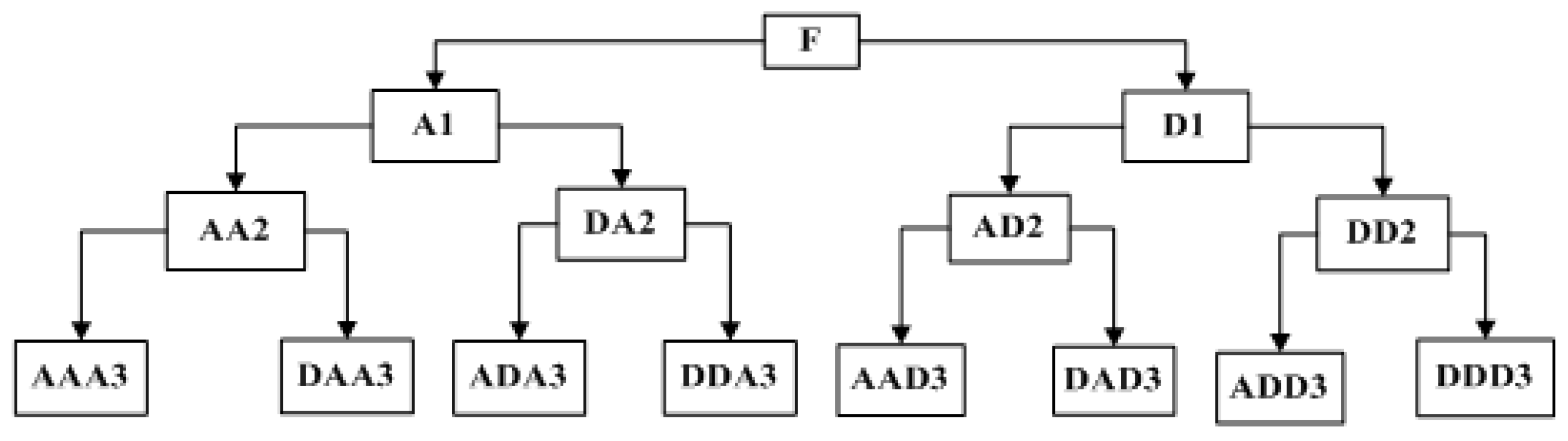
2.3.1. Basic Principles of Wavelet Packet Transform

Wavelet packet transform is the improvement of wavelet transform. It can provide more detailed analysis capability for noisy signal by re-decomposing the high frequency part without subdivision in wavelet transform, so it can further distinguish the PD pulse from the noise signal. According to the double-scaling equation satisfied by wavelet function $\psi (t)$ and orthogonal scaling function $\varphi (t)$, let $u_0(t)=\varphi (t)$ and $u_1(t)=\psi (t)$, the equation becomes:

$$\{\begin{array}{l}{u}_0(t)=\sqrt{2}{\displaystyle \sum _{k}h(k)u_0(2t-k)}\\ u_1(t)=\sqrt{2}{\displaystyle \sum _{k}g(k)u_0(2t-k)}\end{array}$$

(13)

where $g(k)$ and $h(k)$ are the low-pass and high-pass filter coefficients in the multi-resolution analysis, respectively.

Then the $u_n(t)$ can be deduced by recursive relation

$$\{\begin{array}{l}{u}_{2n}(t)=\sqrt{2}{\displaystyle \sum _{k}h(k)u_n(2t-k)}\\ u_{2n+1}(t)=\sqrt{2}{\displaystyle \sum _{k}g(k)u_n(2t-k)}\end{array}$$

(14)

Define the function set ${\left\{u_n(t)\right\}}_{n\in Z}$ as the wavelet packet in terms of $u_0(t)=\varphi (t)$. From the perspective of signal filtering, wavelet packet decomposition is to filter the signal through a set of low-pass filters $H$ and a set of high-pass filters $G$, and obtain a set of low-frequency signals and a set of high-frequency signals after decomposition. So, the wavelet packet transform is to solve the wavelet packet coefficients, wavelet packet decomposition is to solve $\left\{d_l^{j,2n}\right\}$ and $\left\{d_l^{j,2n+1}\right\}$ from $\left\{d_l^{j+1,n}\right\}$ by Equation (12), wavelet packet reconstruction is to solve $\left\{d_l^{j+1,n}\right\}$ from $\left\{d_l^{j,2n}\right\}$ and $\left\{d_l^{j,2n+1}\right\}$ by Equation (13).

$$\begin{array}{l}{d}_l^{j,2n}={\displaystyle \sum _k{h}_{k-2l}{d}_k^{j+1,n}}\\ d_l^{j,2n+1}={\displaystyle \sum _k{g}_{k-2l}{d}_k^{j+1,n}}\end{array}\}$$

(15)

$$d_l^{j+1,n}={\displaystyle \sum _k\left[h_{l-2k}{d}_k^{j,2n}+g_{l-2k}{d}_k^{j,2n+1}\right]}$$

(16)

The process of wavelet packet decomposition is shown in Figure 2 in which the decomposition scale is J = 3. In the figure, F denotes an original signal, D1 denotes a high-frequency component of the first scale decomposition, A1 denotes a low-frequency component of the first-scale decomposition; DA2 denotes a high-frequency component of the second-scale decomposition, and AA2 denotes a low-frequency component of the second scale, the rest can be done in the same manner.

2.3.2. Selection of Wavelet Base and Scale

According to the wavelet packet decomposition principle, it can decompose the high and low frequency signals into corresponding components to perform local time-frequency analysis. In order to ensure the non-redundancy of signal decomposition and reduce the loss of PD signal, it is necessary to select an appropriate decomposition scale. In order to better preserve the characteristics of signal, it is necessary to select the best wavelet base. The threshold function and the compactness are used as the preferred indicators to find the best wavelet base. Through sufficient simulations, the minimum energy loss is achieved by the db4 wavelet base due to the maximum similarity between the db4 wavelet base and the PD signal acquired by HFCT. So, the db4 wavelet base is used for separation of signal and noise in this paper.

As mentioned above, the decomposition scale J in wavelet packet decomposition will affect the decomposition depth and the decomposition result largely. In order to illustrate this point, the single-exponential attenuation signal as described in (17) with white noise is used to simulate the cable partial discharge signal [13] to evaluate the effect of decomposition scale.

$$f(t)=A{e}^{-(t-t_0)/\tau }$$

(17)

where A is the amplitude of PD signal, $t_0$ is the time of PD occurred, $\tau$ is the attenuation coefficient.

When the SNR is −13 dB, different decomposition scales J are set respectively (J = 1,2,3,4) for wavelet packet decomposition. In order to quantitatively analyze the influence of the scale on de-noising effect, the normalized correlation coefficient (NCC) of the first six components and the input noisy PD signal, ${\rho }_k$, the NCC of the first component and the simulated real PD signal, the SNR of de-noised PD signal, and the relative amplitude error, are calculated synchronously. The results are shown in

Table 1. Results at different decomposition scales.

J	${\mathit{\rho }}_1$	${\mathit{\rho }}_2$	${\mathit{\rho }}_3$	${\mathit{\rho }}_4$	${\mathit{\rho }}_5$	${\mathit{\rho }}_6$	NCC	SNR	D (%)
J = 1	0.794	0.608					0.6744	−0.1 dB	10.0
J = 2	0.672	0.424	0.414	0.446			0.7741	2.6 dB	16.7
J = 3	0.446	0.251	0.251	0.230	0.210	0.238	0.8294	4.6 dB	23.3
J = 4	−2.5 × 10−4	−0.006	1.8 × 10−4	−6.2 × 10−4	0.002	0.066	0.8229	4.8 dB	43.3

.

It can be seen from Table 1 that as the decomposition scale increases, the correlation coefficient between each component and the noisy signal decreases, especially when the decomposition scale is 4, the correlation coefficient decreases sharply, which is called over decomposition. It is obvious that, when the decomposition scale is 1, the relative amplitude error is small, but the similarity with the simulated signal is low, which means the relative poor ability of noise suppression. When the decomposition scale is 4, the noise suppression ability is better, but the relative error is large. When the decomposition scale is 3, a better balance between noise suppression and similarity is achieved. Therefore, the three-scale decomposition of the wavelet packet is optimal in terms of the noisy PD signal with the SNR of −13 dB.

Based on the above analysis, a scale adaptive wavelet packet decomposition algorithm for noisy PD signal is employed in this paper. Firstly, according to the signal characteristics, the wavelet base is determined as db4. Perform the decomposition from the minimum scale. If the correlation coefficient between each component and the original signal is less than the given threshold (usually with the threshold value of 0.3 in practice), then stop the decomposition, otherwise increase the scale, continue to decompose until the conditions are met.

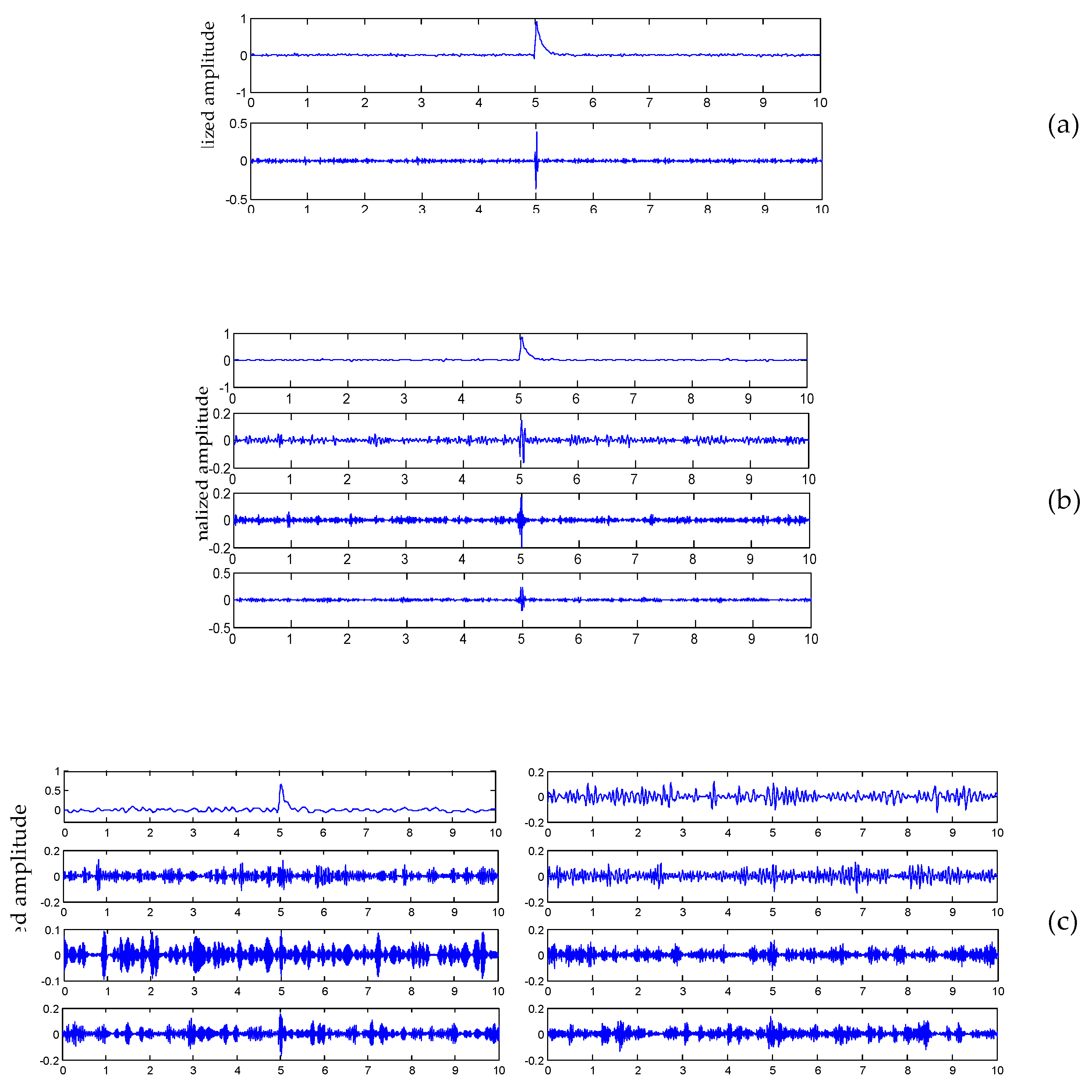
2.3.3. Performance Analysis of Adaptive Wavelet Packet Decomposition for Noisy PD Signal

Different levels of white noises are mixed with the simulated PD signals to generate noisy signals with SNR of 0dB, −2.5 dB, and −13 dB, the decomposition results using the adaptive wavelet packet decomposition mentioned above are shown in Figure 3.

As shown in Figure 3, under different levels of white noise interference, the proposed scale adaptive wavelet packet decomposition achieves good balance of noise suppression and waveform distortion by selecting appropriate scale. In order to explain the results quantitatively, further calculation of NCC and SNR are shown in

Table 2. Quantitative evaluation results of adaptive wavelet packet for different levels of noise.

Parameter	Signal1	Signal2	Signal3
SNR of noisy signal (dB)	0.0	−2.5	−13.0
NCC	0.9507	0.9397	0.8294
SNR of de-noised signal (dB)	10.2	9.4	4.6

.

As shown in Table 2, the adaptive wavelet packet decomposition can suppress white noise effectively in the case of small energy loss, at the same time, the waveform distortion between the extracted PD signal and the simulated real signal waveform is quite small.

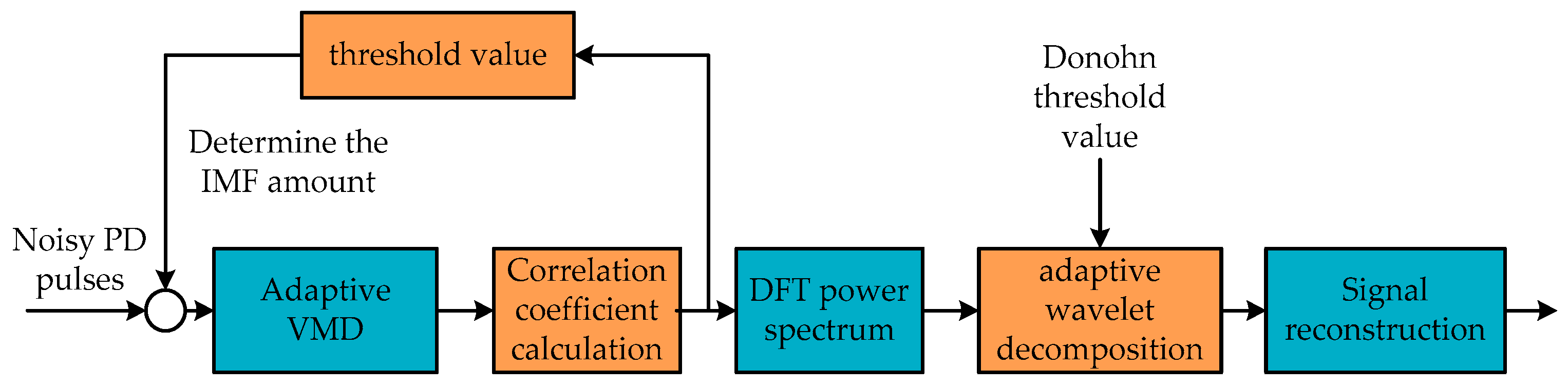
2.4. Proposed De-Noising Method for Complex Noisy PD Signal

PD signal is usually expressed by four mathematical models: Single exponential decay function, double exponential decay function, single exponential oscillation attenuation function, and double exponential oscillation attenuation function. Due to the great oscillation and attenuation of PD signal during the propagation along the cable, the model of single exponential oscillation attenuation and double exponential oscillation attenuation shown in (18) and (19) are employed to describe the PD signal in power cable.

$$f(t)=A{e}^{-(t-t_0)/\tau }\sin \left(2\pi f_c\left(t-t_0\right)\right)$$

(18)

$$f(t)=A\left(e^{-1.3(t-t_0)/\tau }-e^{-2.2(t-t_0)/\tau }\right)\sin \left(2\pi f_c\left(t-t_0\right)\right)$$

(19)

where A is the signal amplitude, which is 1 mV and 5 mV, respectively, here, $\tau$ is the attenuation coefficient, which is 1 $\mu s$ here, $f_c$ is oscillation frequency, taking 5 MHz, $t_0$ is the delay time. The sample frequency is set as 100 MHz, sample time as 40 $\mu s$ at this frequency.

Two kinds of cable PD pulses mentioned above are shown in Figure 4a. To simulate the actual situation, two type noises are added in PD signal. White noise interference with a SNR of −4 dB is added. Since the narrowband interference is mainly sinusoidal or cosine waveform, the sinusoidal function of different frequencies can be used for superposition to simulate the periodic narrowband interference. The frequencies of narrowband interference are set to 1 MHz, 10 MHz, 15 MHz, and the amplitudes are 2 mV, 1 mV, and 0.5 mV, respectively. The PD signal polluted by the two kinds of noise is shown in Figure 4b. The synthetical SNR of the noisy PD signal is −21.4 dB, which can’t be recognized in the time domain.

For the noisy PD signal $g(x)$ synthesized above, its DFT is defined as:

$$G(i)={\displaystyle \sum _{n=0}^{N-1}g(n)e^{-j\frac{2\pi }{N}in}(i=0,1,\dots ,N-1)}$$

(20)

Its power spectrum can be calculated as:

$$P(i)=\frac{1}{N}{\left|G(i)\right|}^2$$

(21)

where $N$ is the data length, $g(n)$ is the sample point.

The DFT power spectrum of PD signal, periodic narrowband component, and white noise component is shown in Figure 5. It’s easy to find that the amplitude of the DFT power spectrum of narrowband interference is much larger than that of the real PD signal and the white noise.

To deal with complex noises with different characteristics, a novel two-step de-noising framework is proposed in which each noise is rejected respectively by appropriate algorithm according to their specific advantages. Because the VMD can decompose an input signal into an ensemble of BLIMFs with the minimal sum of estimated bandwidths for each mode, we employ its instinctive advantage to separate narrowband noise from the input signal firstly. Decompose the noisy PD signals by fast adaptive VMD proposed in Section 2.2, then calculate the DFT power spectrum for each intrinsic mode. According to the fact that the amplitude of the narrowband interference is much larger than the distortion peak of the real PD signal and the white noise power, we remove the mode with narrowband periodic noise, then synthesize the remaining modes for further processing. This middle result is shown in Figure 6a. Secondly, adaptive wavelet packet decomposition proposed in Section 2.3 is employed to remove the component containing white noise according to the threshold method [24], and the remaining components are synthesized as the de-noising PD signal, which is shown in Figure 6b.

As shown in Figure 6c,d, the de-noising PD signal extracted by the proposed method combined adaptive VMD and adaptive wavelet packet decomposition maintains a high degree of similarity with the original signal in amplitude and phase. In order to analyze the results quantitatively, evaluation parameters such as NCC, SNR, and variational trend parameter (VTP) [22] is calculated in

Table 3. Evaluation results of the proposed de-noising method.

Signal	NCC	SNR	VTP
Pulse 1	0.9816	13.39 dB	1.0886
Pulse2	0.9970	19.44 dB	1.0879
Total	0.9886	15.51 dB	1.1166

. VTP represents the similarity of the two waveforms’ changing trends, and measures the oscillation of the waveforms to a certain extent. It makes up for the deficiency of NCC in microscopic description of waveform. The closer VTP is to 1, the more similar the oscillations of the two waveforms are.

From the results shown in Table 3, the extracted PD signals maintain a high degree of similarity with the real signal, the similarity is as high as 0.9977. The waveform detail variational trends also maintains a high degree of consistency, which is up to 1.0485. The SNR after noise suppression reaches the highest level of 14.1 dB, compared with −21.4 dB before de-noising. All these results indicate that adaptive VMD combined with adaptive wavelet packet decomposition method can effectively suppress periodic narrowband and white noise interference.

The specific steps of the proposed de-noising method are given as follows, and the overall flow of our method is shown in Figure 7.

Step 1: Use adaptive VMD algorithm to decompose periodic narrowband signal, white noise signal and partial discharge signal into different intrinsic modal components.

Step 2: Remove the component with the larger power according to the DFT power spectrum, and synthesize the remaining components.

Step 3: The signal obtained in Step 2 is further decomposed by adaptive wavelet decomposition to decompose the white noise into high, medium, and low frequencies.

Step 4: According to the wavelet threshold, remove white noise, synthesize the remaining components as the extracted PD signal.

3. Results and Discussion

3.1. Comparison of De-Noising Results

In order to demonstrate the effect of the proposed method, the CEEMD-based method [26], VMD—wavelet packet method [27], and ours are employed, respectively, to suppress the noise interference described in Section 2, the results of the three methods are shown in Figure 8.

From Figure 8, it is easy to find that, due to the serious frequency aliasing, the CEEMD algorithm can distort the waveform after using the threshold method. In the VMD threshold method, because the threshold cannot be changed according to the noise, the result still contains a large number of noise components. The proposed method takes advantage of VMD to remove periodic narrowband interference, and employs wavelet packet decomposition to remove the residual white noise. The noise level in extracted PD signal is greatly reduced, and the waveform has a high consistency with the simulation waveform. Quantitative results of different method are shown in

Table 4. Quantitative results of different methods.

Method	Evaluation Parameter	Pulse 1	Pulse 2	Total
CEEMD	NCC	0.3847	0.4387	0.3908
	SNR(dB)	0.6752	0.8935	0.7166
VMD wavelet threshold method	NCC	0.6677	0.8100	0.5509
	SNR(dB)	−0.2551	3.0568	3.0239
Proposed method	NCC	0.9816	0.9970	0.9886
	SNR(dB)	13.3906	19.4398	15.5064

.

It can be seen from Table 4 that the proposed method in this paper has the best ability to suppress complex noise. For pulse 1 and pulse 2, it achieves SNR of 13.3906 and 19.4398, respectively, which are much high than other two methods. The extracted PD signal has the highest similarity with the simulated signal, especially the double exponential decay signal, up to 0.9970, and the distortion is small. The results are obviously better than the other two methods, because the proposed adaptive variational mode decomposition can separate periodic narrowband component with high-efficiency. In summary, the method proposed in this paper can better suppress the noise and extract the PD signal in the online cable monitoring system.

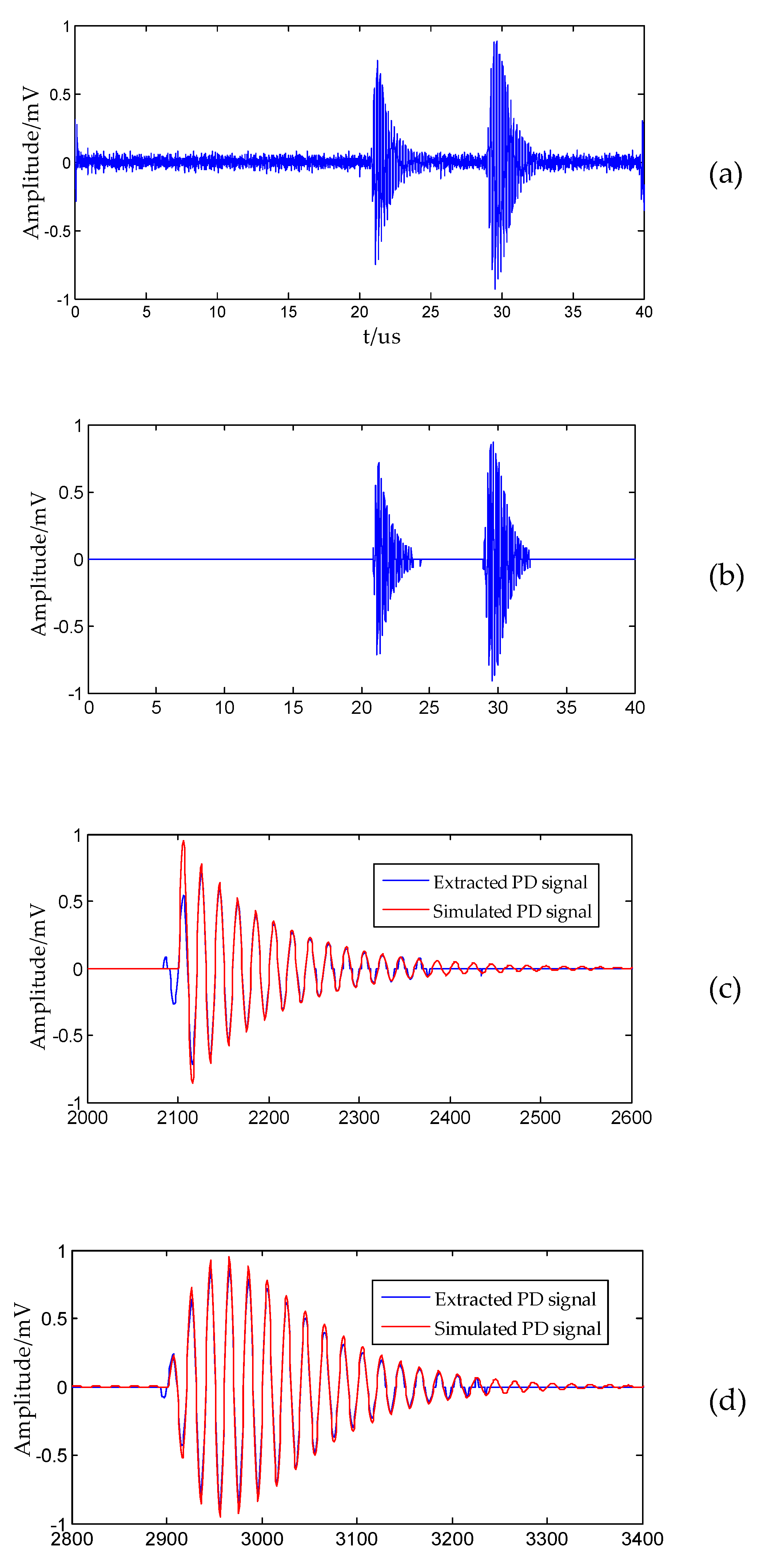
3.2. Robust Estimation of Arrival Time of PD Pulse

In the online PD localization system, due to complex noises, the robustness and accuracy of the estimation of arrival time is not high, and it results in a large localization error. To this end, the proposed two-step de-noising method in Section 2 is used to suppress the noise of the detected on-site PD signal, extract a relatively pure PD signal, and then accurately estimate the first arrival time via the time varying kurtosis algorithm [11,28]. Among the sequences containing PD pulses, the steepness of the signal is the most serious at the moment of pulse onset. Kurtosis is a classical statistic based on high order statistics, which can provide more comprehensive information than low order statistics. It reflects the concentration degree of asymmetric and non-gaussian time sequence, and its value can indicate the steepness of the signal.

Given the random variable $X$, $p\left(X\right)$ is the probability density of $X$, then its kurtosis can be defined as:

$$M=\frac{m_4}{{\left(m_2\right)}^2}-3$$

(22)

where $m_k$ is the k-order statistic of random variable $X$.

According to formula (22), kurtosis value only represents the overall steepness of the signal, and cannot reflect the real-time change of the steepness of time-varying signal. Therefore, time-varying kurtosis algorithm should be further adopted. In the discrete sequence $X\left(i\right)$ to be detected, a sub-time window with length $b$ and sampling point $i$ as the center is designed, the kurtosis value of the signal in the sub-time window is obtained according to formula (22), and time-varying kurtosis value is defined according to the following formula:

$$M_t(i)=\frac{M(i)-M}{M}$$

(23)

where $M$ is the kurtosis of $X\left(i\right)$, and $M\left(i\right)$ is the kurtosis of sub-time window.

In practical applications, the collected PD pulse is sparse. If time-varying kurtosis is obtained on all data sequences, it will not only take time, but also store too much data. The time window energy ratio method was adopted for pretreatment here. The time window $\left[x_n\right]$ where the PD event occurred was determined first, and then the time-varying kurtosis was calculated within the time window. For the time sequence $X\left(i\right)$, take the sampling point $i$ as the center, and take a time window with the neighborhood of $\pm l$. The energy ratio of the rear window and the front window is defined as the energy ratio of the time window.

$$R(i)=\left[{\left({\displaystyle \sum _{k=i}^{i+l-1}{x}_k^2}\right)}^{1/2}\right]/\left[{\left({\displaystyle \sum _{k=i-l}^{i-1}{x}_k^2}\right)}^{1/2}+\lambda \right]$$

(24)

The threshold value of PD event is set, and the time window energy ratio R is compared with the threshold value to determine whether there is PD event in the window. If $R$ is less than the threshold, no PD event occurs in the window, and then cycle to the next moment. If it is larger than the threshold value, the time window with this time as the center and the length $2l$ as the PD time window to pick up the first PD pulse by the time-varying kurtosis.

Time-varying kurtosis curves were drawn for the de-noising signal in Figure 8c and the corresponding noisy signal in Figure 4b, as shown in Figure 9. The first arrival time of PD pulse in Figure 4b is picked up at the 400 sampling point manually, and the maximum value of the time-varying kurtosis curve for the de-noising partial discharge signal is 400, which is consistent with the manual pick-up result. The maximum value of the kurtosis curve is at 794 sampling point of the noisy signal, indicating that it is no longer possible to pick up the first arrival time. In summary, the proposed de-noising method in this paper combines the adaptive VMD and wavelet packet decomposition could extract PD signal effectively from complex noise in practice.

4. Conclusions

In this paper, a novel two-step de-noising method for effectively extracting random PD pulse from complex and strong interferences is proposed and applied to robustly estimate the arrival time of the noisy PD pulse in power cables. Firstly, an improved adaptive VMD is presented to remove out periodic narrowband interference due to its advantage of minimal sum of estimated bandwidths for each mode decomposed from input noisy signal. To avoid over-decomposition or mode loss, the correlation coefficient method is used to determine the optimal intrinsic mode number adaptively. In order to effectively filter out white noise, a scale adaptive wavelet packet decomposition method based on correlation coefficient is proposed, which decomposes the signal into high, middle, and low-frequency components. The components with low frequency, small amplitude are removed out as the white noise interference according to the threshold method, and the residual is the de-noising PD signal. Simulation results show that the proposed method can robustly suppress the interference of periodic narrowband signal and white noise and effectively preserve the essential characteristics of the real PD signal. In the multi-sensor travelling wave based localization system using time-varying kurtosis, accurate estimation of first arrival time of PD pulse can be achieved by the de-noising results.

References

1. Orton, H. Power cable technology review. High Voltage Eng. 2015, 41, 1057–1067. [Google Scholar]
2. Gargari, S.M.; Wouters, P.A.A.F.; Wielen, P.C.J.M.; Steennis, E.F. Partial discharge parameters to evaluate the insulation condition of on-line located defects in medium voltage cable networks. IEEE Trans. Dielectr. Electr. Insul. 2011, 18, 868–877. [Google Scholar] [CrossRef]
3. Wu, R.N.; Chang, C.K. The use of partial discharges as an online monitoring system for underground cable joints. IEEE Trans. Power Del. 2011, 26, 1585–1591. [Google Scholar] [CrossRef]
4. Li, J.H.; Han, X.T.; Liu, Z.H.; Yanming, L. Review on partial discharge measurement technology of electrical equipment. High Voltage Eng. 2015, 41, 2583–2601. [Google Scholar]
5. Babaee, A.; Shahrtash, S.M. On-line partial discharge defected phase selection and localization in cross-bonded single core cables. IEEE Trans. Dielectr. Electr. Insul. 2015, 22, 2995–3006. [Google Scholar] [CrossRef]
6. Álvarez, F.; Garnacho, F.; Ortego, J.; Sánchez-Urán, M.Á. Application of HFCT and UHF sensors in on-line partial discharge measurements for insulation diagnosis of high voltage equipment. Sensors. 2015, 15, 7360–7387. [Google Scholar] [CrossRef] [Green Version]
7. Xu, Y.; Gu, X.; Liu, B.; Hui, B.; Ren, Z.; Meng, S. Special requirements of high frequency current transformers in the on-line detection of partial discharges in power cables. IEEE Elect. Insul. Mag. 2016, 32, 8–19. [Google Scholar] [CrossRef]
8. Hu, X.; Siew, W.H.; Judd, M.D.; Peng, X. Transfer function characterization for HFCTs used in partial discharge detection. IEEE Trans. Dielectr. Electr. Insul. 2017, 24, 1088–1096. [Google Scholar] [CrossRef] [Green Version]
9. Mohamed, F.P.; Siew, W.H.; Soraghan, J.J.; Strachan, S.M.; McWilliam, J. Partial discharge location in power cables using a double ended method based on time triggering with GPS. IEEE Trans. Dielectr. Electr. Insul. 2013, 20, 2212–2221. [Google Scholar] [CrossRef]
10. Choi, W.; Kim, J.; Seo, I.; Hwang, J.; Koo, J. Development of a partial discharge detection algorithm and verification test for extra-high-voltage cable system. IET Sci. Meas. Technol. 2016, 10, 111–119. [Google Scholar] [CrossRef]
11. Sun, K.; Guo, J.; Yang, Y. On Line Partial Discharge Detection and Localization Based on AIC Criterion and Time-Window Energy Ratio. Chin. J. Sens. Actuators 2017, 30, 1209–1214. [Google Scholar]
12. Herold, C.; Leibfried, T. Advanced signal processing and modeling for partial discharge diagnosis on mixed power cable systems. IEEE Trans. Dielectr. Electr. Insul. 2013, 20, 791–800. [Google Scholar] [CrossRef]
13. Jian, X.U.; Cheng-Jun, H. Research on improved fast Fourier transform algorithm applied in suppression of discrete spectral interference in partial discharge signals. Power Syst. Technol. 2004, 28, 80–83. [Google Scholar]
14. Lu, Y.; Han, Z.; Chen, Y. FFT narrowband filtering method based on energy-ratio pretreatment. J. Southeast Univ. 2010, 40, 948–951. [Google Scholar]
15. Zhou, X.; Zhou, C.; Kemp, I.J. An improved methodology for application of wavelet transform to partial discharge measurement denoising. IEEE Trans. Dielectr. Electr. Insul. 2005, 12, 586–594. [Google Scholar] [CrossRef]
16. Mohammadi, F.; Zheng, C.; Su, R. Fault Diagnosis in Smart Grid Based on Data-Driven Computational Methods. In Proceedings of the 5th International Conference on Applied Research in Electrical, Mechanical, and Mechatronics Engineering, Tehran, Iran, 24 January 2019. [Google Scholar]
17. Strela, V.; Heller, P.N.; Strang, G. The application of multi-wavelet filter banks to image processing. IEEE Trans. Image Proc. 2009, 8, 548–563. [Google Scholar] [CrossRef] [Green Version]
18. Li, Y.; Wei, H.; Billings, S.A. Identification of Time-Varying Systems Using Multi-Wavelet Basis Functions. IEEE Trans. Control Syst. Technol. 2011, 19, 656–663. [Google Scholar] [CrossRef]
19. Zhang, Y.; Duan, W.; Li, T. A Reverse Separation Method of Suppressing Periodic Narrowband Noise in Partial Discharge Signal. Trans China Electrotech. Soc. 2015, 30, 232–239. [Google Scholar]
20. Wu, Z.; Huang, N. Ensemble empirical mode decomposition: A noise-assisted data analysis method. Adv. Adaptive Data Anal. 2009, 1, 1–41. [Google Scholar] [CrossRef]
21. Yuan, N.; Zhu, Y.L.; Liang, H.Q. EEMD denoising method using rectangular window. Proc. CSU-EPSA 2015, 27, 54–58. [Google Scholar]
22. Sun, K.; Zhang, J.; Shi, W.; Guo, J. Extraction of Partial Discharge Pulses from the Complex Noisy Signals of Power Cables Based on CEEMDAN and Wavelet Packet. Energies 2019, 12, 3242. [Google Scholar] [CrossRef] [Green Version]
23. Dragomiretskiy, K.; Zosso, D. Variational mode decomposition. IEEE Trans. Signal Proc. 2014, 62, 531–544. [Google Scholar] [CrossRef]
24. Liu, C.; Wu, Y.; Zhen, C. Rolling bearing fault diagnosis based on variational mode decomposition and fuzzy C means clustering. Proc. CSEE 2015, 35, 3358–3365. [Google Scholar]
25. Zhu, Y.; Jia, Y.; Wang, L. Feature extraction and classification on partial discharge signals of power transformers based on improved variational mode decomposition and Hilbert transform. Trans. China Electrotech. Soc. 2017, 32, 221–235. [Google Scholar]
26. Pan, Y.; Zhang, X.; Zhang, Y. Denoising Method for Transformer Partial Discharge Signals Based on Complete Ensemble Empirical Mode Decomposition. Guangdong Electr. Power 2017, 30, 93–98. [Google Scholar]
27. Jiao, S.; Shi, W.; Liu, Q. Self-adaptive partial discharge denoising based on variational mode decomposition and wavelet packet transform. In Proceedings of the 2017 Chinese Automation Congress (CAC2017), Jinan, China, 20 October 2017; pp. 7301–7306. [Google Scholar]
28. Mohammadi, F.; Zheng, C. A Precise SVM Classification Model for Predictions with Missing Data. In Proceedings of the 4th National Conference on Applied Research in Electrical, Mechanical Computer and IT Engineering, Tehran, Iran, 4 October 2018; pp. 3594–3606. [Google Scholar]
Figure 1. Multi-sensor installation. Three sensors A, B, and C are installed on the cable body, where A and B are located at both ends of the measurement interval, and C is located at the midpoint of the AB segment. HFCT: high-frequency current sensor.
Applsci 10 01641 g001
Figure 2. Schematic diagram of three-scale wavelet packets decomposition. F denotes an original signal, D1 and A1 denote the high-frequency and low-frequency component of the first scale decomposition respectively; DA2 and AA2 denote the high-frequency and low-frequency component of the second-scale decomposition, respectively.
Applsci 10 01641 g002
Figure 3. Adaptive wavelet packet decomposition results of different noisy signals. (a) Noisy signal with 0 dB. (b) Noisy signal with −2.5 dB. (c) Noisy signal with −13 dB.
Applsci 10 01641 g003
Figure 4. Simulate cable partial discharge (PD) signals. (a) Clear cable PD signal. (b) Noisy cable PD signal.
Applsci 10 01641 g004
Figure 5. Discrete Fourier transformation (DFT) power spectrum of different components in noisy pulse.
Applsci 10 01641 g005
Figure 6. De-noising results of the proposed method. (a) Result of adaptive variational mode decomposition (VMD). (b) Further result of adaptive wavelet packet de-noising. (c) Comparison of de-noising and real PD signal of pulse 1. (d) Comparison of de-noising and real PD signal of pulse 2.
Applsci 10 01641 g006
Figure 7. The overall flow of the proposed de-noising method.
Applsci 10 01641 g007
Figure 8. De-noising results by different methods. (a) Result of the CEEMD-based method. (b) Result of VMD—wavelet packet method. (c) Result of the proposed method.
Applsci 10 01641 g008aApplsci 10 01641 g008b
Figure 9. Time-varying kurtosis curves before and after noise suppression. (a) Curve of noisy PD signal. (b) Curve of de-noising PD signal.
Applsci 10 01641 g009