Aerodynamic Characteristics of Different Airfoils under Varied Turbulence Intensities at Low Reynolds Numbers

Featured Application

The study of airfoil affected by the unsteady jet flow of turboelectric distributed propulsion aircraft was conducted, which lays a good foundation for future design of turboelectric distributed propulsion (TeDP) unmanned aerial vehicles (UAVs).

Abstract

A numerical study was conducted on the influence of turbulence intensity and Reynolds number on the mean topology and transition characteristics of flow separation to provide better understanding of the unsteady jet flow of turboelectric distributed propulsion (TeDP) aircraft. By solving unsteady Reynolds averaged Navier-Stokes (URANS) equation based on C-type structural mesh and $\gamma -{\widetilde{\mathrm{Re}}}_{\theta t}$ transition model, the aerodynamic characteristics of the NACA0012 airfoil at different turbulence intensities was calculated and compared with the experimental results, which verifies the reliability of the numerical method. Then, the effects of varied low Reynolds numbers and turbulence intensities on the aerodynamic performance of NACA0012 and SD7037 were investigated. The results show that higher turbulence intensity or Reynolds number leads to more stable airfoil aerodynamic performance, larger stalling angle, and earlier transition with a different mechanism. The generation and evolution of the laminar separation bubble (LSB) are closely related to Reynolds number, and it would change the effective shape of the airfoil, having a big influence on the airfoil’s aerodynamic characteristics. Compared with the symmetrical airfoil, the low-Reynolds-number airfoil can delay the occurrence of flow separation and produce more lift in the same conditions, which provides guidance for further airfoil design under TeDP jet flow.

1. Introduction

The research over the last several years on the fixed-wing unmanned aerial vehicles (UAVs) with turboelectric distributed propulsion (TeDP) has attracted much attention. The most representative ones are X-57, ESAero, GL-10, N3-X, E-airbus, and many other models [1,2]. The TeDP system is used to provide lift when UAVs take off. Due to the driving of the distributed propulsion to the air, the flow behind the propulsion system grows extremely complex, which is not only accelerated, but also with strong turbulence. Meanwhile, the characteristic Reynolds number of the wing becomes ultra low because the freestream velocity is almost zero. Owing to the influence of the turbulence and low Reynolds number, the three-dimensional effect of the wing becomes more complicated, which means the wing would encounter the coupling of up and down wash flow, flow separation, laminar separation bubble, spanwise vortex and other phenomena [3,4,5,6].

Different from the laminar flow in which the fluid elements keep parallel to each other, the turbulent flow makes the fluid elements in the irregular vortex motion, and the mixing of different size eddies causes strong exchange and transmission of energy and heat, rapid dissipation of mechanical energy [7,8]. Turbulent flow is three-dimensional, rotational, intermittent, highly disordered, diffusive and dissipative. The actual modes of turbulence are eddies and high-vorticity regions, so that turbulence is often described by eddy viscosity as a local property of the fluid [9]. Generally, it is considered that the turbulence intensity less than or equal to 1% is low-intensity turbulence, and the turbulence intensity greater than 10% is high-intensity turbulence. In the wind tunnel experiment, the turbulence intensity of the inflow is usually within 3%, but in the practical application, the turbulence intensity near the propulsion system is often more than 5%. When the flow is affected by a small fan’s wake and atmospheric turbulence, the turbulence intensity could usually be greater than 10% [10]. Due to the existence of a large number of mixed jets in the combustion chamber and complex cooling structure in the combustor liner, the turbulence intensity at the outlet of the aeroengine could be 15%–20% [11]. Therefore, in the face of the complex jet flow behind the UAV with TeDP, it is very important to study the aerodynamic characteristics of the two-dimensional airfoil under varied turbulence intensities and low Reynolds numbers (Re < 5 × 10⁵).

Under a low Reynolds number, the current study of turbulence intensity mainly focuses on the flow near a flat plate. Gramespacher [12] carried out experiments to study the influence of flow homogeneity and isotropy, decay of turbulent kinetic energy, energy spectra, and length scales. Grzelak [13] investigated the isotropy and homogeneity of turbulence through skewness and kurtosis of the flow velocity distribution function and transverse variation. He also studied the impact of turbulence intensity on bypass laminar–turbulent transition parameters on a flat plate through experiments. Hancock [14] confirmed an appreciably nonlinear dependence of the skin-friction coefficient and other boundary layer parameters on RMS freestream turbulence intensity. Hiller [15] found that the mean flow-field responds strongly to turbulence intensity but with little effect of integral scale, and fluctuating pressures depend strongly upon both intensity and scale. Fransson [16] and Jacobs [17] observed the formation of streamwise oriented streaks in the separated shear layer, which significantly altered the flat plate boundary-layer transition under high levels of turbulence intensity. Marxen [18] analyzed the transition mechanism by observing the development of small disturbances and their role in the final breakdown to turbulence through direct numerical simulation (DNS). McAuliffe [19] conducted a numerical simulation of transition under low and high disturbance. The study examines the role of the velocity profile shape on the instability characteristics and the nature of the large-scale vortical structures shed downstream of the bubble and enables identification of the structure of the instability mechanism and the characteristic structure of the resultant turbulent spots.

The research on the effect of turbulence intensity on airfoil is mostly concentrated on the turbine blade and low-speed airfoil. Lengani [10] found that the free-stream turbulence intensity modify the transition and separation processes of the suction side boundary layer of a highly loaded low pressure turbine blade through experiment. The stall characteristics of airfoil S1223 has been investigated by Cao [20] at low Reynolds numbers, implying that the smaller integral length under 4.1% turbulence intensity delays the boundary layer separation on the suction surface. Mistf [21] conducted an experiment of NACA0015 immersed in two grid generated homogenous flows. Istvan [22,23] investigated NACA0018 under varied Reynolds numbers and turbulence intensities to find that increasing freestream turbulence intensity results in earlier transition and reattachment, contributing to an overall decrease in separation bubble length. Bryan [24] established an extensive database of surface oil flow measurements of seven airfoils that represents a wide range in behavior at low Reynolds numbers. Wang and Li [25,26] carried out an experiment on NACA0012 under varied turbulence intensities at Re =5,300 to validate their numerical simulation. Arunvinthan [27] studied the aerodynamic characteristics of unsymmetrical airfoil at various turbulence intensities through experiments and found that the lift coefficient increases with the increase of turbulence intensity. The results also reveal that the flow featuring turbulence can effectively delay the stall characteristics of an airfoil by attaching the flow over the airfoil for an ex-tended region. The influence of freestream turbulence intensity (FSTI) level on the structure and dynamic properties of a laminar separation bubble has been experimentally studied by Simoni [28]. He concluded that the bubble length and height reduction at a high FSTI level with a fixed Reynolds number are due to the higher amplitude of velocity fluctuations penetrating into the separating boundary layer. Conversely, the Reynolds number significantly influences the time-mean boundary layer structure at separation.

The existing research on the influence of the turbulence intensity on airfoils have been conducted with Reynolds numbers between 100,000 and 1200,000, but the work under 100,000 Reynolds number is lacking. Meanwhile the TeDP UAV is a new topic, which brings about new problems in airfoil design. It is necessary to carry out further research on aerodynamic performance of airfoil in the flow with great changes of Reynolds number and turbulence intensity. Therefore, facing the unsteady jet flow generated by the TeDP system during taking off, the aerodynamic performance of airfoil under varied Reynolds numbers and turbulence intensities is studied by using the commercial software FLUENT based on the computational fluid dynamics (CFD) method. The numerical method applied in this paper is verified by comparing the pressure distribution, the lift and drag coefficient of the NACA0012 airfoil with different turbulence intensities and Reynolds numbers. The effects of turbulence intensity and Reynolds number on the aerodynamic performance of airfoil and flow field characteristics are studied. The mechanisms of earlier transition in the boundary layer, the relationship between the evolution of laminar separation bubble and Reynolds number are presented.

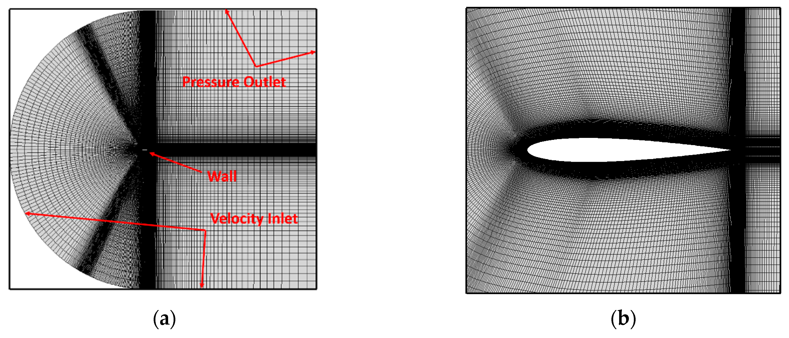
2. Numerical Approach

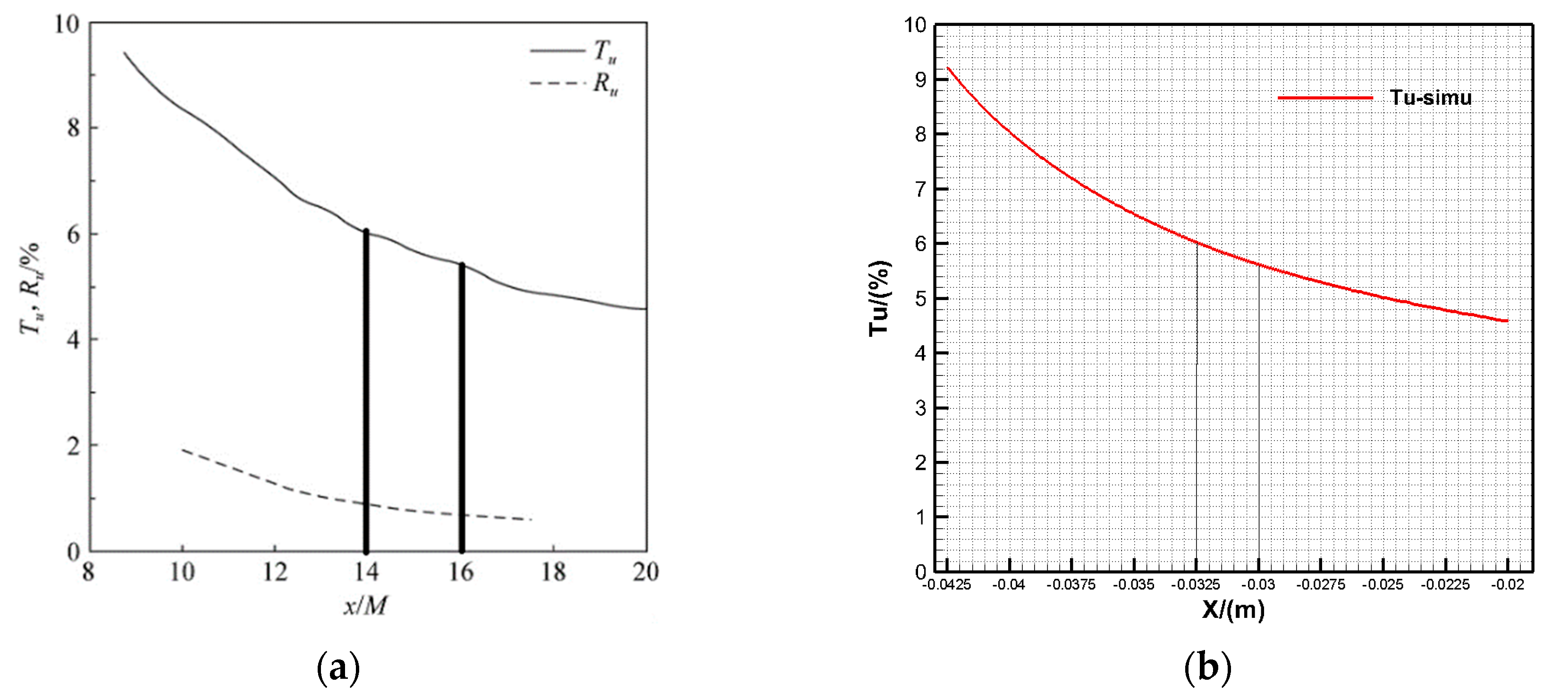
2.1. Estimation Method of Turbulence Intensity

Turbulence intensity (Tu) is a physical quantity to measure the degree of irregular motion of fluid element. Turbulence intensity is defined as the ratio of the rms of fluctuating velocity u’ to average velocity $\overline{U}$(Equation (1))

$$\mathit{Tu}=\frac{\sqrt{\overline{{u^{\prime }}^2}}}{\overline{U}}$$

(1)

In turbulent flow, the mean values of velocity and pressure are easy to observe, while the fluctuating velocity can be measured by precise hot wire anemometer, laser velocimeter and particle image velocimetry. The turbulence energy is mainly concentrated in the large-scale eddy structure, which is related to the turbulence length scale l. The characteristic length of turbulence depends on the geometric length and has a decisive influence on the development of turbulence. If the flow at the entrance is restricted by the wall and has a turbulent boundary layer, the turbulent length scale can be calculated by l = 0.4δ_99%, where the δ_99% is the thickness of boundary layer. As for the flow affected by the inlet grid, the turbulence length scale is approximately equal to the grid aperture, namely l ≈ d. [6,21].

R_T is the ratio of turbulence viscosity to laminar viscosity, which is directly proportional to the turbulent Reynolds number. In the high-Reynolds-number boundary layer, shear layer and fully developed pipe flow, the turbulence viscosity ratio is large, about 100–1000. However, in most free flow boundary layers, the turbulence viscosity ratio is quite small, usually 1–10.

It is observed in a relative static wind tunnel that the turbulent flow behind the grid of the wind tunnel is steady, and its intensity is continuously attenuated along the flow direction from the inlet of the experimental section. According to the reference [29], the relationship between the turbulence attenuation and the increase of flow direction distance can be described as follows:

$$Tu=T{u}_{inlet}{\left(1+R{e}_{x}1.5\beta \frac{T{u}_{inlet}{}^2}{R_{T,inlet}}\right)}^{-{\beta }^{\ast }/2\beta }$$

(2)

In the numerical simulation, the attenuation of turbulence intensity can be more directly reflected by the turbulent dissipation rate ε (Equation (3)).

$$\epsilon ={\beta }^{\ast }{}_{}^{3/4}\frac{k^{3/2}}{l}$$

(3)

where k is turbulent kinetic energy, $\beta$ and ${\beta }^{\ast }$ are the empirical constants in the turbulence model. The values are β = 0.0828, β* = 0.09.

2.2. $\gamma -{\widetilde{\mathrm{Re}}}_{\theta t}$ Transition Model

The $\gamma -{\widetilde{\mathrm{Re}}}_{\theta t}$ transition model is based on the local variables of flow field proposed by Langtry and Menter, in which the intermittence factor γ and the transition momentum thickness Reynolds number ${\widetilde{\mathrm{Re}}}_{\theta t}$ are added to construct the transport equations. The γ is used to depict the flow characteristics of the transition region, which represents the probability of turbulence at a point in flow field, and the value range is 0 ≤ γ ≤ 1. ${\widetilde{\mathrm{Re}}}_{\theta t}$ is used to control the generation of intermittence factors and to form a criterion for predicting the starting position of transition.

Transport equation of γ is:

$$\frac{\partial \left(\rho \gamma \right)}{\partial t}+\frac{\partial \left(\rho U_j\gamma \right)}{\partial x_j}=P_{\gamma 1}-E_{\gamma 1}+P_{\gamma 2}-E_{\gamma 2}+\frac{\partial }{\partial x_j}\left[\left(\mu +\frac{{\mu }_j}{{\sigma }_j}\right)\frac{\partial \gamma }{\partial x_j}\right]$$

(4)

Transition source term and fracture/laminar fluidization source term are defined as follows:

$$P_{\gamma 1}=C_{a1}{F}_{length}\rho S{\left[\gamma F_{onset}\right]}^{C\gamma 3}$$

(5)

$$E_{\gamma 1}=C_{e1}{P}_{\gamma 1}\gamma$$

(6)

$$P_{\gamma 2}=C_{a2}\rho \Omega \gamma F_{turb}$$

(7)

$$E_{\gamma 2}=C_{e2}{P}_{\gamma 2}\gamma$$

(8)

where S is strain rate, F_length is the empirical correlation for controlling the length of transition region, $\Omega$ is vorticity, the constant terms are C_a1 = 2, C_e1 = 1, C_a2 = 0.06, C_e2 = 50, C_γ3 = 0.5.

The vorticity Reynolds number is defined as:

$${\mathrm{Re}}_v=\frac{\rho y^{2}S}{\mu }$$

(9)

The other parameters are as below:

$$R_T=\frac{\rho k}{\mu \omega }$$

(10)

$$F_{onset1}=\frac{{\mathrm{Re}}_v}{2193{\mathrm{Re}}_{\theta c}}$$

(11)

$$F_{onset2}=\min \left(\max \left(F_{onset1},F_{onset}^4\right),2.0\right)$$

(12)

$$F_{onset3}=\max \left(1-{\left(\frac{R_T}{2.5}\right)}^3,0\right)$$

(13)

$$F_{onset}=\max \left(F_{onset2}-F_{onset3},0\right)$$

(14)

$$F_{turb}=e^{-{\left(\frac{R_T}{4}\right)}^4}$$

(15)

The transport equation of $\gamma -{\widetilde{\mathrm{Re}}}_{\theta t}$ is:

$$\frac{\partial \left(\rho {\widetilde{\mathrm{Re}}}_{\theta t}\right)}{\partial t}+\frac{\partial \left(\rho U_j{\widetilde{\mathrm{Re}}}_{\theta t}\right)}{\partial x_j}=P_{\theta t}+\frac{\partial }{\partial x_j}\left[{\sigma }_{\theta t}\left(\mu +{\mu }_t\right)\frac{\partial {\widetilde{\mathrm{Re}}}_{\theta t}}{\partial x_j}\right]$$

(16)

The source term is defined as:

$$P_{\theta t}=c_{\theta t}\frac{\rho }{t}\left({\mathrm{Re}}_{\theta t}-{\widetilde{\mathrm{Re}}}_{\theta t}\right)\left(1.0-F_{\theta t}\right)$$

(17)

The coupled equation with the shear stress transport (SST) flow model is:

$$\frac{\partial }{\partial t}\left(\rho k\right)+\frac{\partial }{\partial x_j}\left(\rho u_{j}k\right)=\frac{\partial }{\partial x_j}\left[{\Gamma }_k\frac{\partial k}{\partial x_j}\right]+G^{\ast }{}_k-Y^{\ast }{}_k+S_k$$

(18)

$$G^{\ast }{}_k={\gamma }_{eff}{\tilde{G}}_k$$

(19)

$$Y^{\ast }{}_k=\min \left(\max \left({\gamma }_{eff},0.1\right),1.0\right)Y_k$$

(20)

Other parameters are defined by reference [30,31,32].

3. Validation of Numerical Simulation Method

The numerical calculation is based on unsteady Reynolds averaged Navier-Stokes (URANS) equations coupling with the $\gamma -{\widetilde{\mathrm{Re}}}_{\theta t}$ transition model. The semi-implicit method for pressure-linked equations consistent (SIMPLEC [33,34]) scheme was used for the pressure-velocity coupling. The discretized momentum and pressure correction equations are solved implicitly, whereas the velocity correction is solved explicitly, thus resulting in a semi-implicit method. Second order upwind spatial discretization was used for all variables, in combination with the least square cell-based method for the gradients. The time step is determined by Strouhal number (Sr) (Equation (21)), which is a similarity criterion to characterize the unsteady flow.

$$Sr=\frac{fc}{U}$$

(21)

where the f is the frequency of unsteady period of motion, c the chord length of airfoil, and U the velocity of flow.

The generation of computational mesh and boundary conditions are shown in Figure 1. The computational mesh is divided by C-type structural mesh. The radius of calculation field is 50 times of the chord length.

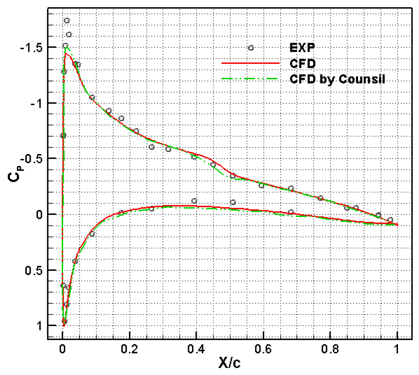
3.1. Validation of Pressure Distribution

Referring to reference [35], the numerical simulation of the NACA0012 airfoil at Reynolds number of 250,000 is carried out. The FSTI in experiment is Tu = 0.58%. The angle of attack (AoA) of the airfoil is α = 4°, and the chord length is c = 0.3048 m. The calculation condition is consistent with the experiment. The quantity of computational mesh is about 100,000 cells, and the first layer grid element to wall distance is d₁ = 2.03 × 10⁻⁵c, y⁺ = 0.25. The inflow velocity is V = 11.982 m/s.

Solutions are considered sufficiently converged when the order of magnitude of the residuals is low and remains constant. Figure 2 shows the assessment between the experiments and the results of the CFD, where the CFD by Counsil represents numerical solution calculated in reference [36].

Figure 2 shows that, the numerical simulation of the pressure distribution fits well with the experiment result, and describes the separation and reattachment process well. In addition, the CFD results are consistent with those given by Counsil. It shows that the calculation method is accurate to predict the transition process.

3.2. Validation of Aerodynamic Force

Referring to reference [25], the numerical simulation of the NACA0012 airfoil at ultra-low Reynolds number of 5,300 is carried out. The range of the angle of attack of the airfoil is α = 0°–25°, chord length of airfoil is c = 0.1 m. The experiment is conducted in a water tunnel, and the water flow velocity is U = 0.053 m/s. Because the experimental velocity of the water tunnel is too small, the incompressible flow condition is transformed into low-speed incompressible air flow according to the criterion of Reynolds similarity. The size of the airfoil is scaled to 1/40 of the original size, namely c’ = 0.0025 m. The inflow velocity of air inlet boundary is V = 30.96 m/s.

In order to verify the influence of the quality of computation mesh, five angles of attacks of the NACA0012 airfoil were calculated and compared with the experimental values. Figure 3 represents the assessment between the experiments and the results of the CFD computations with three different meshes: 52,500 (coarse), 73,000 (medium), and 95,000 (fine) cells.

The results of the mesh dependency study is shown in

Table 1. Results of the mesh independency study. AOA: angle of attack; R: ratio of errors between Fine and Exp.

AOA	Coarse	Medium	Fine	Exp	R
2	0.1324	0.1256	0.1123	0.098	0.146
5	0.3276	0.3207	0.2950	0.282	0.046
8	0.6323	0.6218	0.6224	0.612	0.017
10	0.7314	0.7421	0.7507	0.785	0.044
12	0.7231	0.7748	0.7893	0.856	0.078

. Exp represents the experiment results, R the ratio of errors between Fine and Exp. All lift coefficients converged monotonically for all angles of attack and the value of R is less than 0.15. As illustrated in Figure 3, the numerical results obtained with the fine mesh predicted the experimental lift well. Therefore, this higher resolution mesh was used for the current computations. It should be noted that because the due to value of lift at 2° angle of attack is small, the error of the numerical calculation result is relatively large. The computational mesh contains 95,000 cells, and the first layer grid element to wall distance is d₁ = 6.53 × 10⁻⁴c, y⁺ = 0.25.

A definite curve of the decay law of experimental turbulence intensity at Tu = 6% is given in reference [25], as is shown in Figure 4a. The range between airfoil leading edge and trailing edge is X/M = 14–16. A decay law of turbulence intensity curve is fitted by changing turbulence scale and turbulent dissipation rate in numerical calculation and is shown in Figure 4b, where the range between airfoil leading edge and trailing edge is X = −0.0325–−0.03.

The comparison between the numerical and experimental results of different turbulence intensities is depicted in Figure 5. Figure 5a indicates that the lift coefficient fits well within the angle of attack of 10° at Tu = 6%. As the angle of attack increases, there is no definite stall phenomenon at α = 12°–15°, which is slightly different from the experimental results. As a result of the lack of corresponding decay law of experimental turbulence intensity at Tu = 0.6%, the calculation error is large. Even so, the trends of the lift and drag coefficients are consistent with the experimental results.

The airfoil characteristics are further analyzed in the following section. In this paper, the numerical simulation is implemented with an unsteady method, but the figures such as the streamline diagram, turbulent kinetic energy diagram, pressure distribution diagram, friction drag diagram and so on, deal with a time-averaged method. All numerical data are the time-averaged results of 50 time steps after convergence. Figure 6 shows the comparison of pressure distribution of the airfoil at different turbulence intensities and angles of attack.

The pressure distribution shows that: there are few differences in pressure distributions at α = 5°, and the overall trend of pressure distribution is relatively approximate (Figure 6a). As for the pressure distribution at Tu = 0.6%, the upper and lower surface pressure coefficients tend to be consistent about 50%c, resulting in the loss of lift contribution from this position to the trailing edge. However, there are significant differences in pressure distributions between Tu = 6% and Tu = 0.6% at α = 10° and α = 15° (Figure 6b,c). At Tu = 6%, the pressure distribution changes sharply for the both angles of attack. A pressure bulge is generated at about 20%c and 10%c respectively, which is similar to that of the classical separation bubble, and is quite different from that of the flow separation at high angle of attack. At Tu = 0.6%, the premature separation of the flow results in a rapid attenuation of the suction peak near the leading edge of the airfoil, and the pressure coefficient near 5%c keeps almost constant until the trailing edge, which indicates that the high turbulence intensity has a certain inhibitory effect on the flow separation.

A further comparison of turbulent kinetic energy and streamline around the airfoil corresponding to Tu = 6% and Tu = 0.6% is conducted in the following figures (Figure 7 and Figure 8). The streamlines in the figures clearly reflect the aerodynamic characteristics of the flow field.

It can be seen that: At α = 5°and Tu = 6%, the flow separation only occurs near the trailing edge of the airfoil, and the streamline adheres well at other positions; At α = 10°, the separation begins near 20%c of the upper surface of the airfoil and reaches to the trailing edge. The topology of the separation vortex is more similar to the characteristics of the classical laminar separation bubble (LSB) separation as mentioned earlier. With the increase of the angle of attack, the scale of the separation vortex becomes larger and the separation point is advanced, but the center of the separation vortex is still within the chord range of the airfoil. When the turbulence intensity is 0.6%, the flow separation region expands as the angle of attack increases. At α = 5°, the flow separation occurs near 45%c of its upper surface. At α = 15°, the streamline begins to separate near 5%c of the upper surface, and there is no reattachment after the flow separation. The center of the separation vortex is located outside the chord of the airfoil, forming a typical high-attack-angle separation.

The magnitude of turbulent kinetic energy represents the intensity of turbulence. When transition occurs in the boundary layer, the turbulent kinetic energy would increase sharply. Comparing the streamline and turbulent kinetic energy under two turbulence intensities, it can be found that when the airfoil is at the same angle of attack, the flow corresponding to the large turbulence intensity is more stable, and the flow separation area is smaller. This means that the larger turbulence intensity can inject the high energy from the freestream into the turbulent shear layer, and the fluid elements can overcome some adverse pressure gradient to make the flow separation restrained.

From the above, it can be seen that the numerical simulation method adopted in this paper is applicable to the calculation of complex flow under varied low Reynolds numbers and turbulence intensities, which meets the application of airfoil design under the jet flow of TeDP UAV.

4. Effect of Turbulence Intensity on Airfoil at Different Reynolds Numbers

Considering the variability of the jet flow of TeDP aircraft affects the aerodynamic performance of the wing, the effect of turbulence intensity and Reynolds number on airfoil is studied in the following section. As stated earlier, there is quite a lot of research of for Reynolds number between 100,000 and 1200,000. Thus, Re₁ = 26,500 and Re₂ = 53,000 are chosen for further research, and the state of Re₃ = 212,000 is calculated as a complement. In addition, since NACA0012 is a popular symmetric airfoil, the SD7037 airfoil is selected for comparison. The SD7037 airfoil has a relative thickness of t/c = 9.20% and a relative camber of f/c = 3.02%. It operates at a low Reynolds number and it is favored for R/C model sailplanes because of its working lift range (the lift range over the low drag region) that begins near a C_L of 0.2 and extends to near C_L of 1.0 where the drag begins to increase more rapidly [37]. During the calculation, the turbulence intensity at the leading edge of airfoils is guaranteed to be Tu = 6% and Tu = 0.6%. The lift and drag characteristics are shown in Figure 9 and Figure 10.

Generally, the flow around airfoils is complex in the range of Re = 10,000–100,000. There may be laminar boundary layer, laminar separation, transition, turbulent boundary layer and turbulent separation. It can be seen from Figure 9 and Figure 10 that under Tu = 6% corresponding to states of Re₁ = 26,500 and Re₂ = 53,000, the lift coefficient increases linearly with small angle of attack. At Re₂ = 53,000, the stalling angle of NACA0012 is 12°, while that of SD7037 is 15°. This shows that the SD7037 airfoil has better lift characteristics. At Tu = 0.6%, the lift coefficient is evidently nonlinear and the stalling angle is smaller for both of the airfoils. At Re₁ = 26,500, the stalling angle of both airfoils decreases to only 8°, and there is a sharp increase of drag around α = 10°. Figure 11 also indicates that the pressure drag of the airfoil suddenly increases at α = 10°, which may be the result of the development of the flow separation with the increase of the angle of attack. At Re₃ = 212,000, the lift coefficient of both airfoils increases further, and the stalling phenomenon delays, which is more evident at Tu = 0.6%. Notably, at α = 2° and α = 5°, the lift coefficient of the airfoil at Tu = 0.6% is bigger than that at Tu = 6%, which might have something to do with the generation of the LSB.

In the aspect of drag, Figure 11a (in which C_D,p represents the coefficient of pressure drag, C_D,f the coefficient of friction drag) indicates that the NACA0012 airfoil has a small pressure drag at small angle of attack. With the angle of attack increasing to 15°, the airfoil stalls and the pressure drag increases sharply at Tu = 0.6%. Besides, in comparison with a high level of turbulence intensity, the frictional drag is smaller at Tu = 0.6%. The variation of drag characteristics of the SD7037 airfoil is similar to NACA0012 (Figure 11b).

Generally, as for a specific Reynolds number, the increasing freestream turbulence intensity results in a minor decrease in lift at small angle of attack, whereas at pre-stall angle of attack and higher turbulence intensity levels, lift increases and stall is delayed, as stated in [22]. Similarly, at a specific turbulence intensity, the increasing Reynolds number results in improvement of aerodynamic performance of airfoil, and the enhancement of the ability of the boundary layer to resist the adverse pressure gradient. Compared with NACA0012, the lift characteristics of the SD7037 airfoil are better, while the drag coefficient is slightly higher. Winslow [6] also concluded that below the Reynolds number of 10⁵, cambered airfoils have better lift and drag characteristics than thick conventional airfoils with rounded-leading edges.

The differences of airfoil aerodynamic characteristics under the influence of different Reynolds numbers and turbulence intensities will be further analyzed in the following section.

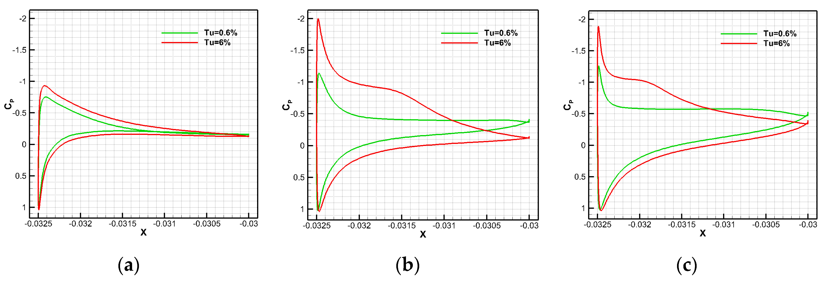
4.1. The Influence of Turbulence Intensity Upon Airfoils at Re₁ = 26,500

At Re₁ = 26,500, the aerodynamic characteristics of airfoils were analyzed at angles of attack of 5°, 8° and 10°. The pressure distribution and chordwise friction drag coefficient (C_f,X) of airfoils in varied turbulence intensities is shown in Figure 12 and Figure 13.

Analyzing the pressure coefficient and friction coefficient under different turbulence intensities, together with the details of the corresponding flow field (Figure 14, Figure 15, Figure 16 and Figure 17), it can be seen that:

At α = 5°, the surface pressure distribution curve of the NACA0012 airfoil is smooth at Tu = 6%, indicating that the flow is stable and the streamline adheres well (Figure 12a and Figure 14a). While the boundary layer on the upper surface of SD7037 airfoil begins to separate at about 82%c and reattached near the trailing edge, forming a separation bubble (Figure 16a). However, because the separation bubble is small, the airfoil pressure distribution does not change significantly. At Tu = 0.6%, the pressure distribution of the NACA0012 airfoil around 30%–60%c on the upper surface forms a pressure platform. The C_f,X becomes negative at 18%c, which indicates that the flow is separated (Figure 13a and Figure 15a). The streamline around NACA0012 wraps a slender eddy due to the laminar separation (Figure 15a). The SD7037 airfoil also experiences flow separation, but the separation point is slightly delayed, at about 25%c (Figure 17a).

When the angle of attack of the airfoils increases to 8°, flow separation occurs near the trailing edge of the NACA0012 airfoil at Tu = 6%, and a separation bubble forms near the trailing edge of the SD7037 airfoil (Figure 13b and Figure 16b). At Tu = 0.6%, flow separation occurs near 4%c on the upper surface of NACA0012 airfoil, and the separation area extends to the trailing edge (Figure 15b). Similarly, flow separation occurs near 14%c on the upper surface of SD7037 airfoil (Figure 17b). With the angle of attack increasing to 10°, at Tu = 6%, a slender separation bubble is generated around 3%–16%c on the upper surface of the NACA0012 airfoil, and the flow separation area near the trailing edge is expanded (Figure 14c). The location of trailing edge separation bubble on the SD7037 airfoil is slightly advanced, and a longer separation bubble is formed near 8%–20%c. At Tu = 0.6%, the pressure distribution platform on the upper surface of the two airfoils appears earlier. The flow separation has the characteristics of separation bubbles in terms of pressure distribution.

From the evolution of flow separation on the upper surface of the airfoils at Tu = 0.6% can be concluded that the increasing angle of attack results in the increase of adverse pressure gradient around the trailing edge, contributing to the separation of the boundary layer. Then the separation point moves towards the leading edge until the complete high-attack-angle separation, and stall happens. However, the airfoil’s aerodynamic performance improves and the process of separation is suppressed at Tu = 6%. In general, the greater turbulence outside the boundary layer enhances flow stability, injects energy into the upstream laminar flow around the airfoil, and enhances the ability to resist adverse pressure gradients, so that the laminar flow separation could be delayed or overcome. Then, the high-energy fluid in the freestream is brought to the near-wall area in the flow mixing process, which strengthens the stability of the turbulent shear layer to overcome the adverse pressure gradient, making it possible for the flow to reattach to the airfoil surface.

In addition, compared with the NACA0012 airfoil, the SD7037 airfoil has greatly delayed the occurrence of transition and flow separation due to its good low-Reynolds-number performance, ensuring better adhesion of the boundary layer, and thus obtaining greater lift and stalling angle. And the flow reattaches to form a trailing edge separation bubble on the upper surface of the SD7037 at Tu = 6%, which is different from that of the NACA0012.

4.2. The Influence of Reynolds Number on the Airfoil

The effect of Reynolds number on airfoils has been discussed a lot in the literature. The main discussion here is on the airfoil aerodynamic performance with an increasing Reynolds number in terms of the improvement of stalling angle, generation of LSB, and the earlier transition. The pressure distribution and chordwise friction drag coefficient of airfoils with an angle of attack of 10° in varied turbulence intensities at Re₂ = 53,000 are shown in Figure 18.

It can be seen that flow separation, transition, and a short LSB occur around the leading edge of NACA0012 under both turbulence intensities at Tu = 0.6%, as well as SD7037. There is no appearance of separation or LSB on the upper surface of SD7037 at Tu = 6%, but Figure 18b shows that the transition still exists. In addition, combined with Figure 13c and Figure 18, it can be seen that: With the increase of Reynolds number, the high-attack-angle separation around the trailing edge on the upper surface transfers to a small separation section, and the degree of flow separation is restrained. This shows that with the increase of Reynolds number, the shear effect on the airfoil surface is enhanced, the kinetic energy is more abundant, and the ability to resist the adverse pressure gradient is enhanced, so that the airfoil aerodynamic performance and stalling angle improves.

Figure 19 shows the transformation of chordwise friction drag coefficient at angles of attack of 8° under three different Reynolds numbers.

Taking the NACA0012 at Tu = 0.6% as an example, it can be seen that with the increase of Reynolds number, an earlier separation occurs on the upper surface of airfoil, the separation point transfers from 5%c to 2%c, and reattaches to the wall around 22%c, forming a typical structure of short LSB. When the Reynolds number increases to Re₃ = 212,000, the position of the LSB transfers to 6%–13%c, and the size of the LSB becomes evidently smaller. In addition, the valley value of C_f,X represents the onset of laminar flow transition, and peak value after the valley of C_f,X represents the finish of the transition to turbulent flow. Figure 19 shows that the transition point moves forward from 42%c through 17%c to 12%c, and the reattachment point also moves forward from 80%c through 25%c to 13%c. It can be concluded that, the increasing Reynolds number results in earlier transition and reattachment, contributing to an overall decrease in separation bubble length, as stated in [38].

In addition, the generation of the LSB affects the aerodynamic characteristics of the airfoils. The pressure distribution and chordwise friction drag coefficient of airfoils with an angle of attack of 5° in varied turbulence intensities at Re₂ = 53,000 are shown in Figure 20.

It can be seen that transition occurs on the upper surface of both airfoils and then laminar separation bubbles form at Tu = 0.6%. The generation of the laminar separation bubble changes the effective shape of the airfoil, increases the curvature of the upper surface of the airfoil (Figure 20c) so that the lift coefficient of the airfoil at Tu = 0.6% is bigger than that at Tu = 6%, and also causes the nonlinear phenomenon of the lift coefficient at small angle of attack as shown in Figure 9a and Figure 10a. However, when the separation bubble size is small or forms near the trailing edge of the airfoil, it has little effect on the lift characteristics of the airfoil.

5. Discussion

Through the comparison of the aerodynamic performance of different airfoils with different turbulence intensities and Reynolds numbers, it is found that the flow field around the airfoil is very unstable under low Reynolds number conditions, and the flow phenomenon on the suction side of the airfoil is abundant. The effects of turbulence intensity mainly appeared to be that with the increase of turbulence intensity, the aerodynamic performance of airfoil becomes more stable, the lift improves, the stalling angle increases, and the occurrence of an LSB or flow separation can be suppressed to a certain extent.

The numerical results show that under low Reynolds number conditions, the level of the turbulence intensity determines the flow characteristics (The external factors such as surface roughness and noise are not considered in this paper). In the fully developed turbulent boundary layer, most of the velocity fluctuation originate from the average shear flow, which is reflected in the production term of the turbulent kinetic energy equation. If the freestream turbulence is strong, the higher velocity fluctuations outside the boundary layer diffuse into the boundary layer near the airfoil surface. The intensity of this diffusion effect directly determines the occurrence of the transition. If the freestream turbulence is weak, the occurrence of transition is hardly affected by external disturbances, but basically caused by the instability of its inner flow so that external disturbances are only as a trigger. Mayle [39] pointed out that when the freestream turbulence intensity is higher than 3%, the effect of pressure gradient on the transition can be ignored. Transition is mainly affected by external disturbances. When the turbulence intensity is less than 1%, the pressure gradient and shear flow dominate the stability of flow. And the occurrence of transition at turbulence intensity of 1%–3% is affected by both external and inner factors such as freestream turbulence intensity and pressure gradient.

The increase of the Reynolds number also causes the transition to move towards the leading edge, so that the lift and stalling angle increase, but the mechanism of the earlier transition is different from that of turbulence intensity. The increase of turbulence intensity leads to an earlier transition because of the higher velocity fluctuations that penetrate within the boundary layer. However, the increase of the Reynolds number alters the state of the boundary layer at separation reducing the shear layer thickness and consequently its stability characteristics. Simoni [28] also concluded that the Reynolds number significantly influences the time-mean boundary layer structure at separation. This translates into higher growth rates and different dynamic properties of the shedding phenomenon.

In addition, the evolution of the LSB structure on the suction side of the airfoil is closely related to the Reynolds number. Taking the medium angle of attack (α = 8°) of the NACA0012 airfoil at Tu = 0.6% as an example, at Re₁ = 26,500, an eddy similar to a long laminar separation bubble emerges on the upper surface of the airfoil, but fails to reattach to the wall. At Re₂ = 53,000, a small short laminar separation bubble is generated near the leading edge. At Re₃ = 212,000, an LSB occurs on the upper surface of the airfoil near the trailing edge. These phenomena show that the generation of separation bubbles is closely related to the Reynolds number if the Reynolds number is too small, the laminar flow is not able to reattach to the wall after the transition, and it is difficult to form an LSB. As the Reynolds number increases, a complete LSB structure arises and the morphology of the LSB alters from a long separation bubble or a short separation bubble near the leading edge to a separation bubble near the trailing edge of the NACA0012 airfoil. It is worth noting that a separation bubble occurs at the trailing edge of the SD7037 airfoil at Re₁ = 26,500, Tu = 6%, indicating that SD7037 has better low-Reynolds-number aerodynamic performance.

This conclusion is consistent with the empirical criterion given by Carmichael [40]; Under natural laminar flow separation, the distance from flow separation to reattachment can be expressed as Re_R − Re_S = 50,000 (where Re_R is the Reynolds number of reattachment, Re_S is the Reynolds number of separation), which indicates that the separation flow of the airfoil will no longer reattach when the Reynolds number is less than 5 × 10⁴,. Meanwhile, if the Reynolds number is slightly higher than 5 × 10⁴, a separation bubble will occur. Additionally, if the low-Reynolds-number performance of the airfoil is excellent, the reattachment will also occur when the Reynolds number is less than 5 × 10⁴.

6. Conclusions

In this paper, a numerical study was conducted on the influence of turbulence intensity and Reynolds number on the mean topology and transition characteristics of flow separation to provide better understanding of the unsteady jet flow of TeDP UAV. Through the comparative analysis of the aerodynamic performance of the NACA0012 airfoil with experimental results, the numerical calculation method was verified. The effects of turbulence intensity and Reynolds number on aerodynamic performance of different airfoils, transition characteristics and evolution of LSBs were analyzed. The following conclusions are made.

The increasing freestream turbulence intensity results in earlier transition and reattachment. At small angle of attack and higher turbulence intensity levels, airfoil encounters a minor decrease in lift, whereas at pre-stall angle of attack, lift increases and stall is delayed. Similarly, the increasing Reynolds number results in higher local vorticity Reynolds number and smaller flow energy dissipation, contributing to a stronger effect of the overall surface shear and earlier transition. The shear layer around airfoil can resist an adverse pressure gradient for a longer distance so that aerodynamic performance of the airfoil improves. However, the mechanism of earlier transition is different. The increase of turbulence intensity leads to an earlier transition because of the higher velocity fluctuations that penetrate within the boundary layer. However, the increase of the Reynolds number alters the state of the boundary layer at separation, reducing the shear layer thickness and consequently its stability characteristics.

The generation of the LSB in laminar flow usually occurs at a Reynolds number of 50,000 and the evolution of the LSB structure on the suction side of the airfoil is closely related to Reynolds number and turbulence intensity. As the Reynolds number or turbulence intensity increases, the LSB will emerge earlier and its length will become shorter. The generation of the LSB changes the effective shape of the airfoil, and increases the curvature of the suction side of the airfoil, which causes the nonlinear phenomenon of the lift coefficient at small angle of attack. In addition, different airfoils have different sensibility to turbulence intensity and Reynolds number. Compared with the low-speed symmetrical airfoil, the low-Reynolds-number airfoil not only has superior performance in lift characteristics, but also in delaying flow separation. This research provides guidance for further airfoil design of the TeDP UAVs.

References

1. Kong, X.; Zhang, Z. Review of electric power system of distributed electric propulsion aircraft. Acta Aeronaut. Astronaut. Sin. 2018, 39, 51–67. [Google Scholar]
2. Nalianda, D.; Singh, R. Turbo-electric distributed propulsion—Opportunities, benefits and challenges. Aircr. Eng. Aerosp. Technol. 2014, 86, 543–549. [Google Scholar] [CrossRef]
3. Wang, K.; Zhu, X.; Zhou, Z. Distributed electric propulsion slipstream aerodynamic effects at low Reynolds number. Acta Aeronaut. Astronaut. Sin. 2016, 37, 2669–2678. [Google Scholar]
4. Lee, B.J.; Liou, M.F.; Kim, H. Design of distributed mail-slot propulsion system on a hybrid wingbody air-craft, AIAA-2018-3954. In Proceedings of the 2018 Applied Aerodynamics Conference, Atlanta, GA, USA, 25–29 June 2018. [Google Scholar]
5. Gibson, A.; Green, M.; Schiltgen, B. TurboElectric Distributed Propulsion (TeDP) Design, Performance, Bene-fits, Concerns and Considerations for both Conventional Non-Superconducting and Cryogenically Cooled Super-conducting Machines in a Propulsion System Architecture for Conventional Tube-and-Wing Configuration; ISABE: Busan, Korea, 2013. [Google Scholar]
6. Winslow, J.; Otsuka, H. Basic understanding of airfoil characteristics at low reynolds numbers (104–105). J. Aircr. 2017, 55, 1050–1061. [Google Scholar] [CrossRef]
7. Mueller, T.J.; Pohlen, L.J.; Conigliaro, P.E.; Jansen, B.J. The influence of freestream disturbances on low reynolds number airfoil experiments. Exp. Fluids 1983, 1, 3–14. [Google Scholar] [CrossRef]
8. Boiko, A.V.; Grek, G.R.; Dovgal, A.V.; Kozlov, V.V.; Dowling, D.R. Origin of turbulence in near-wall flows. Appl. Mech. Rev. 2003, 56, B13. [Google Scholar] [CrossRef]
9. Argyropoulos, C.D.; Markatos, N.C. Recent advances on the numerical modelling of turbulent flows. Appl. Math. Model. 2015, 39, 693–732. [Google Scholar] [CrossRef]
10. Lengani, D.; Simoni, D. Recognition of coherent structures in the boundary layer of a low-pressure-turbine blade for different freestream turbulence intensity levels. Int. J. Heat Fluid Flow 2015, 54, 1–13. [Google Scholar] [CrossRef]
11. Porté-Agel, F.; Wu, Y.T.; Lu, H. Large-eddy simulation of atmospheric boundary layer flow through wind turbines and wind farms. J. Wind Eng. Ind. Aerodyn. 2011, 99, 154–168. [Google Scholar] [CrossRef]
12. Gramespacher, C.; Albiez, H. The generation of grid turbulence with continuously adjustable intensity and length scales. Exp. Fluids 2019, 60, 85. [Google Scholar] [CrossRef]
13. Grzelak, J. Influence of freestream turbulence intensity on bypass transition parameters in a boundary layer. J. Fluids Eng. 2017, 139, 051201. [Google Scholar] [CrossRef]
14. Hancock, P.E.; Bradshaw, P. The effect of freestream turbulence on turbine boundary layers. J. Fluids Eng. 1983, 105, 284–294. [Google Scholar] [CrossRef]
15. Hillier, R.; Cherry, N.J. The effects of stream turbulence on separation bubbles. J. Wind Eng. Ind. Aerodyn. 1981, 8, 49–58. [Google Scholar] [CrossRef]
16. Fransson, J.H.M.; Matsubara, M. Transition induced by free-stream turbulence. J. Fluids Mech. 2005, 527, 1–25. [Google Scholar] [CrossRef]
17. Jacobs, R.G.; Durbin, P. Simulations of bypass transition. J. Fluids Mech. 2001, 428, 185–212. [Google Scholar] [CrossRef]
18. Marxen, O.; Lang, M.; Rist, U. A Combined experimental/numerical study of unsteady phenomena in a laminar separation bubble. Flow Turbul. Combust. 2003, 71, 133–146. [Google Scholar] [CrossRef]
19. McAuliffe, B.R.; Yaras, M.I. Transition mechanisms in separation bubbles under low- and elevated-freestream turbulence. J. Turbomach. 2010, 132, 011004. [Google Scholar] [CrossRef]
20. Cao, N.; Ting, D.S. The Performance of a high-lift airfoil in turbulent wind. Wind Eng. 2011, 35, 179–196. [Google Scholar] [CrossRef]
21. Mistf, P. Mean loading effects on the surface pressure fluctuations on an airfoil in turbulence: AIAA-2001-2211. In Proceedings of the 7th AIAA/CEAS Aeroacoustics Conference and Exhibit, AIAA, Maastricht, The Netherlands, 28–30 May 2001. [Google Scholar]
22. Istvan, M. Turbulence intensity effects on laminar separation bubbles formed over an airfoil. AIAA J. 2018, 56, 335–1347. [Google Scholar] [CrossRef]
23. Istvan, M.S.; Yarusevych, S. Effects of free-stream turbulence intensity on transition in a laminar separation bubble formed over an airfoil. Exp. Fluids 2018, 59, 52. [Google Scholar] [CrossRef]
24. Bryan, D.; McGranahan, M.; Selig, S. Surface oil flow measurements on several airfoils at low reynolds numbers. AIAA-2003-4067. In Proceedings of the 21st AIAA Applied Aerodynamics Conference, Orlando, FL, USA, 23–26 June 2003. [Google Scholar]
25. Wang, S.; Mi, J. Effect of large turbulence intensity on airfoil load and flow. Acta Aeronaut. Astronaut. Sin. 2011, 32, 41–48. [Google Scholar]
26. Li, S.; Wang, S. Effect of turbulence intensity on airfoil flow: Numerical simulations and experimental measurements. Appl. Math. Mech. 2011, 32, 964–972. [Google Scholar] [CrossRef]
27. Arunvinthan, S.; Nadaraja, S. Aerodynamic characteristics of unsymmetrical aerofoil at various turbulence intensities. Chin. J. Aeronaut. 2019, 32, 2395–2407. [Google Scholar] [CrossRef]
28. Simoni, D.; Lengani, D. Inspection of the dynamic properties of laminar separation bubbles: Free-stream turbulence intensity effects for different Reynolds numbers. Exp. Fluids 2017, 58, 66. [Google Scholar] [CrossRef]
29. Chen, Y. On the Transition Prediction for Aeronautical Application; Northwestern Polytechnical University. Press: Xi’an, China, 2008; Volume 23–35, pp. 44–46. [Google Scholar]
30. Menter, F.R.; Langtry, R.B.; Likki, S.R.; Suzen, Y.B.; Huang, P.G.; Völker, S. A correlation based transition model using local variables Part 1—Model formulation: ASME 2004-GT-53452. In Proceedings of the Turbo Expo 2004: Power for Land, Sea, and Air, Vienna, Austria, 14–17 June 2004. [Google Scholar]
31. Langtry, R.B.; Menter, F.R.; Likki, S.R. A Correlation based transition model using local variables Part 2-Test cases and industrial applications, ASME 2004-GT-53434. In Proceedings of the Turbo Expo 2004: Power for Land, Sea, and Air, Vienna, Austria, 14–17 June 2004. [Google Scholar]
32. Mistf, M.T.; Obayashi, S. Application of local correlation-based transition model to flows around wings, AIAA-2006-918. In Proceedings of the 44th AIAA Aerospace Sciences Meeting and Exhibit, Reston, VA, USA, 9–12 January 2006. [Google Scholar]
33. Jang, D.S.; Jetli, R. Comparison of the PISO, SIMPLER, and SIMPLEC algorithms for the treatment of the pressure-velocity coupling in steady flow promblems. Numer. Heat Transf. 1986, 10, 209–228. [Google Scholar] [CrossRef]
34. Shen, W.; Michelsen, J.A. An improved SIMPLEC method on collocated grids for steady and unsteady flow computations. Numer. Heat Transf. 2003, 43, 221–239. [Google Scholar] [CrossRef]
35. Wahidi, R.; Bridges, D. Experimental Investigation of the Boundary Layer and Pressure Measurements on Airfoils with Laminar Separation Bubbles. AIAA-2009-4278. In Proceedings of the 39th AIAA Fluid Dynamics Conference, San Antonio, TX, USA, 22–25 June 2009. [Google Scholar]
36. Counsil, J.N.N.; Goni Boulama, K. Validating the URANS shear stress transport γ −Reθ model for low-Reynolds-number external aerodynamics. Int. J. Numer. Meth. Fluids 2012, 69, 1411–1432. [Google Scholar] [CrossRef]
37. Selig, M.S.; Guglielmo, J.J.; Broeren, A.P.; Giguere, P. Summary of Low-Speed Airfoil Data; SoarTech Publications: Virginia Beach, VA, USA, 1995; Volume 1. [Google Scholar]
38. Zhang, Y.; Zhao, K. The influence of Reynolds number on boundary layer development and stall characteristics of airfoil. Adv. Aeronaut. Sci. Eng. 2019, 10, 319–329. [Google Scholar]
39. Mayle, R.E. The role of laminar-turbulent transition in gas turbine engines. ASME J. Turbomach. 1991, 113, 509–537. [Google Scholar] [CrossRef]
40. Carmichael, B.H. Low Reynolds Number Airfoil Survey: NASA CR 1165803; NASA: Washington, DC, USA, 1981. [Google Scholar]
Figure 1. Mesh and boundary conditions. (a) Mesh in farfield; (b) Mesh around airfoil.
Applsci 10 01706 g001
Figure 2. Comparison of numerical calculation and experiment results of pressure distribution. CFD: computational fluid dynamics; EXP: experiment.
Applsci 10 01706 g002
Figure 3. Lift coefficient of numerical simulations versus experiment data of the NACA0012 airfoil.
Applsci 10 01706 g003
Figure 4. Decay law of turbulence intensity along the flow direction. (a) Turbulence intensity change in experiment; (b) Turbulence intensity change in numerical simulation.
Applsci 10 01706 g004
Figure 5. Comparison of numerical calculation and experiment results. (a) CL vs α; (b) CD vs α.
Applsci 10 01706 g005
Figure 6. Airfoil pressure distribution affected by different turbulence intensities at three angles of attack. (a) α = 5°; (b) α = 10°; (c) α = 15°.
Applsci 10 01706 g006
Figure 7. Flow characteristic such as turbulent kinetic energy and streamline shape at Tu = 6%, (a) α = 5°; (b) α = 10°; (c) α = 15°.
Applsci 10 01706 g007
Figure 8. Flow characteristic such as turbulent kinetic energy and streamline shape at Tu = 0.6%, (a) α = 5°; (b) α = 10°; (c) α = 15°.
Applsci 10 01706 g008
Figure 9. Aerodynamic characteristics of NACA0012 at different Reynolds numbers and turbulence intensities. (a) CL vs α; (b) CD vs α.
Applsci 10 01706 g009
Figure 10. Aerodynamic characteristics of SD7037 at different Reynolds numbers and turbulence intensities. (a) CL vs α; (b) CD vs α.
Applsci 10 01706 g010
Figure 11. The component of the drag coefficient of airfoils varies with the angle of attack at different Reynolds numbers and turbulence intensities. (a) NACA0012; (b) SD7037.
Applsci 10 01706 g011
Figure 12. Airfoil pressure distribution affected by different turbulence intensities at three angles of attack. (a) α = 5°; (b) α = 8°; (c) α = 10°.
Applsci 10 01706 g012
Figure 13. Airfoil chordwise skin friction drag coefficient affected by different turbulence intensities at three angles of attack. (a) α = 5°; (b) α = 8°; (c) α = 10°.
Applsci 10 01706 g013
Figure 14. The NACA0012 airfoil characteristics such as turbulent kinetic energy and streamline shape at Tu = 0.6%; (a) α = 5°; (b) α = 8°; (c) α = 10°.
Applsci 10 01706 g014
Figure 15. The NACA0012 airfoil characteristics such as turbulent kinetic energy and streamline shape at Tu = 0.6%, (a) α = 5°; (b) α = 8°; (c) α = 10°.
Applsci 10 01706 g015
Figure 16. The SD7037 airfoil characteristic such as turbulent kinetic energy and streamline shape at Tu = 6%, (a) α = 5°; (b) α = 8°; (c) α = 10°.
Applsci 10 01706 g016
Figure 17. The SD7037 airfoil characteristic such as turbulent kinetic energy and streamline shape at Tu = 0.6%, (a) α = 5°; (b) α = 8°; (c) α = 10°.
Applsci 10 01706 g017
Figure 18. Airfoil aerodynamic performance at α = 10°, Re2 = 53,000. (a) Pressure distribution; (b) Coefficient of chordwise friction drag.
Applsci 10 01706 g018
Figure 19. The chordwise friction drag coefficient of airfoil at α = 8° under the Reynolds number of (a) Re1 = 26,500; (b) Re2 = 53,000; (c) Re3 = 212,000.
Applsci 10 01706 g019
Figure 20. Airfoil aerodynamic performance at α = 5°, Re2 = 53,000. (a) Pressure distribution; (b) Coefficient of chordwise friction drag; (c) Effective shape of NACA0012 at Tu = 0.6%.
Applsci 10 01706 g020