Fast Planar Detection System Using a GPU-Based 3D Hough Transform for LiDAR Point Clouds

Abstract

Plane extraction is regarded as a necessary function that supports judgment basis in many applications, including semantic digital map reconstruction and path planning for unmanned ground vehicles. Owing to the heterogeneous density and unstructured spatial distribution of three-dimensional (3D) point clouds collected by light detection and ranging (LiDAR), plane extraction from it is recently a significant challenge. This paper proposed a parallel 3D Hough transform algorithm to realize rapid and precise plane detection from 3D LiDAR point clouds. After transforming all the 3D points from a Cartesian coordinate system to a pre-defined 3D Hough space, the generated Hough space is rasterised into a series of arranged cells to store the resided point counts into individual cells. A 3D connected component labeling algorithm is developed to cluster the cells with high values in Hough space into several clusters. The peaks from these clusters are extracted so that the targeting planar surfaces are obtained in polar coordinates. Because the laser beams emitted by LiDAR sensor holds several fixed angles, the collected 3D point clouds distribute as several horizontal and parallel circles in plane surfaces. This kind of horizontal and parallel circles mislead plane detecting results from horizontal wall surfaces to parallel planes. For detecting accurate plane parameters, this paper adopts a fraction-to-fraction method to gradually transform raw point clouds into a series of sub Hough space buffers. In our proposed planar detection algorithm, a graphic processing unit (GPU) programming technology is applied to speed up the calculation of 3D Hough space updating and peaks searching.

1. Introduction

In lots of environment perception and terrain analysis applications, accurate plane surfaces are significant information that are researched by lots of scholars [1]. In an outdoor environment, building surfaces are considered as fixed obstacles that assist unmanned ground vehicles (UGVs) to realize local autonomous positioning [2,3]. Besides, plane surface detection is a fundamental function in indoor applications for building modeling and analysis [4].

In most UGVs’ applications, light detection and ranging (LiDAR) sensors are widely utilized to collect high precision point clouds with rich and reliable environment information [5]. In addition to the advantages of LiDAR point clouds (e.g., large-scale, real-time), several disadvantages are not neglected in point cloud processing, including its unstructured, irregular and unsymmetrical spatial distribution, and uneven density. To overcome these disadvantages in plane extraction applications, some researchers proposed pre-processes to balance point cloud density and re-order registration alignment [6]. However, the pre-processes require multiple iterations before executing plane detection so that the time efficiency is affected especially in initial phase [7]. Therefore, the preprocesses of density balancing and re-order registration methods are not adopted in real-time plane surface detection applications [8].

Neighbouring point clustering is a common pre-process method of point clouds to decrease the calculation time [9]. By clustering points with the same normal vector or other spatial characteristics, point groups are regarded as individual computing units to execute the following plane detection procedures. These clustering-based methods are only suitable for a small number of point clouds with a uniform density, whereas LiDAR point clouds collected from outdoor environment are massive and unorganised.

Without a complex pre-process, two main plane detection algorithms are applicable for both indoor and outdoor environments, namely, random sample and consensus (RANSAC) and the three-dimensional Hough transform (3DHT). The initial phase in the fully automatic RANSAC algorithm is totally random, resulting in significant computational and time complexity to traverse a large number of LiDAR point clouds. Because the parameter searching of the plane surface is an entirely stochastic process in the RANSAC algorithm, the Hough transform is more suitable for detecting a plane surface from point clouds when compared with RANSAC [10].

The traditional 3DHT algorithm transforms all 3D points that belong to a whole scene into a pre-defined Hough space buffer. The higher the resolution of the angles and point counts, the more computation time is consumed for Hough space generation. To reduce the time consumption in the traditional 3DHT, this study proposes a parallel 3D Hough transform algorithm for planar detection from LiDAR point clouds. Using a central processing unit (CPU) and graphic processing unit (GPU) hybrid framework, the processing speed performs much faster than that using the CPU method. In (CPU-GPU) addition, for decreasing the disturbance caused by the parallel and horizontal circle distribution of LiDAR point clouds, this paper adopted a fraction-to-fraction method to transform raw points gradually from Cartesian coordinate systems into the Hough space. In this way, the performance of plane surface detection in each frame is improved with a high executing efficiency.

The remainder of this paper is organised as follows. Section 2 surveys some popular methods on 3D plane detection. Section 3 introduces the proposed planar detection system using a GPU-based 3D Hough transform. Section 4 describes the experimental procedures and evaluates the plane detection results. Finally, Section 5 provides the conclusion of the study.

2. Related Works

This section surveys several plane detection methods, including clustering techniques, RANdom SAmple Consensus (RANSAC) and its variants, Hough-like voting methods, and peak searching methods in parameter spaces.

2.1. Clustering Methods

Spatial distribution was a prominent judgmental information to analyse the surface shape features of a 3D point cloud in clustering methods. Liang et al. [11] compared the relative values of eigenvectors and eigenvalues to locate the calibration plane in an indoor environment. Region-growing techniques, which selected a local seed plane and then expanded the plane region by adding its neighbouring points, were also utilised in plane identification. Abdullah et al. [12] utilised seed points that were the nearest to the extracted line centres and neighbouring points to generate a planar surface incrementally. To improve the efficiency, region-growing methods based on Octrees and voxels were exploited, Deschaud et al. [13] applied a voxel growing algorithm to detect a plane and grow a region based on the normal estimation of each point using a filtered weighted plane fitting method. Vo et al. [14] adopted an Octree-based region-growing algorithm on voxelised point clouds to incrementally add the adjacent voxels into a cluster. According to the covariance matrix generated by adjacent unstructured points, subdivision planes were detected in individual sub-spaces [15].

Considering the influence of the outliers and noise in point cloud data, Nurunnabi et al. [16] firstly deleted the outlier data and then fitted the planar surface using a principal component analysis (PCA) algorithm, from which the estimated plane normals and curvatures were exploited to fit the plane. Yeon et al. [17] utilised a divide-and-conquer method to dispose point cloud groups with similar plane parameters based on a robust PCA to improve estimation accuracy. To promote plane detection performance, the majority of the optimisation approaches of the plane extraction algorithm enhanced the filtering efficiency of noise and outlier points in the initial phase and the robustness and stability in the peak searching process.

In these types of plane extraction methods, the neighbouring area should be defined before computing the local geometry features, resulting in a high time consumption of the neighbouring point searching for computing Euclidean or other types of spatial distance. The accuracy rate of plane detection in these methods depends on the sub-space resolution, in which a higher resolution requires more computations. Thus, speed performance and computational complexity are the major difficulties existing in the two main types of plane detection methods.

2.2. Stochastic Methods

RANSAC is a classic stochastic method for plane detection. To optimise the accuracy of the RANSAC algorithm, the components of inliers in [18] were connected and grew into a corresponding plane surface using a RANSAC method. Qian et al. [19] proposed a normal-coherence CC (NCC)-RANSAC algorithm, where a coherence check was performed to remove the data patches whose normal directions were inconsistent with the fitted plane. The clustered planar surfaces consisted of examined inlier patches, which improved the plane extraction accuracy. To increase time efficiency, the modification of the initial situation and restrictive condition is always employed in the RANSAC algorithm to reduce the iteration times during plane extraction. Yue et al. [20] employed a mean shift algorithm to compute normal vectors of point clouds in different segmented voxels as a rough initialisation in the pre-process. Unlike a fully random selection of the beginning points, the estimation of the normal vectors can reduce the iteration times during optimal plane parameter searching. Because many outlier points exist in collected datasets from real outdoor environment, the accuracy rates of plane estimation were hard to maintain in a steady level. To avoid erroneous results caused by outlier points, Li et al. [21] adopted a normal distribution transformation algorithm prior to the execution of the plane surface search. Using the normal vector transform algorithm in the pre-process, unorganised point clouds were converted into alignment representations as a down-sampling method to reduce computational cost. After applying the normal vector transform into the RANSAC algorithm, the time efficiency of plane detection was much higher than that of the standard RANSAC algorithm. Alehdaghi et al. [22] proposed a parallel extension to the RANSAC algorithm that performed GPU cores to extract planes from point clouds.

In the stochastic method, geometry features (e.g., normal) are used to determine the optimal fitting plane through one or multiple times of the point cloud iteration. The satisfied point counts for different plane surfaces are recorded during the iteration process, after which the pairs of the parameters of the optimum plane surface are obtained on the basis of the satisfied points of maximum counts. Owing to the uncertainty and randomness characteristics of these RANSAC related algorithms, its performance is still not suitable for real-time data processing.

2.3. Parameter Spaces Methods

The Hough transform is a classic plane detection algorithm based on parameter space, in which optimal plane parameters are determined by a generated Hough space. Unlike the RANSAC algorithm, the global maximum of point counts can be gained after traversing all of the grid cells in Hough space. Thus, the Hough transform supports more stable plane information than RANSAC when processing non-ideal point cloud datasets. However, the standard Hough transform remains sensitive to noise points and occlusions, wherein the plane detection accuracy considerably depends on the parameters’ resolution of the angle and radius. To improve the anti-interference performance, Vera et al. [23] utilised a Gaussian kernel to generate an accumulator map in the Hough space rather than directly computing the point counts. In addition, a quad tree was also used in their proposed method to group adjacent points as a down-sample procedure during pre-process.

To locate a more reasonable peak from the accumulator map, smoothing and gradient climbing steps were added during the peak searching process to obtain the required plane surface parameters. In the algorithm proposed by Limberger et al. [6], coplanar sample points were firstly clustered by a subdivision procedure to ensure that a kernel-based Hough transform was performed on clusters instead of individual points. Jeltsch et al. [24] applied a regularisation method on the Hough parameter space to correct the computation error caused by different resolutions in horizontal and vertical directions. Using this regularisation method, the line detection results from the point cloud were improved and overcame the problem that more than one lines were extracted from dense points of cylindrical distribution. Maltezos et al. [25] proposed another point cloud down-sampling method to modify the time efficiency of plane parameter computing in the Hough transform algorithm. Using an adaptive resolution model in the point cloud space, a low-level mode was applied at an initial density to gain rough plane parameters. Before employing a high-level mode to calculate precise parameters, a density mask was developed to filter several points in the intensive area to reduce point densities. In the down-sampled point cloud space, accurate plane parameters were gained with robust performance and rapid speed. Similar to the gradient climbing step in the peak searching process, a probabilistic clustering method was employed by Marriott et al. [26] to improve the searching efficiency rate. Moreover, a Gaussian mixture regression model was added in the method to correct distorted planes caused by the environment sensor prior to outlier trimming process.

The most significant advantage of parameter space methods is the stable plane detecting results without random interference. Besides, if the resolution of the Hough space and point counts were fixed, the time complexity of plane detection in every frame is also stable. Our previous work [27] adopted RANSAC algorithm to detect plane surfaces in an outdoor environment using parallel computing technology. We also applied a 2D Hough transform algorithm to detect indoor planar surface in work [28]. Due to the characteristics of LiDAR point cloud, the connectivity information is absent among the unstructured and unorganised points. To extract plane surfaces from a large number of point clouds, parameter space methods have better computation efficiency than the clustering methods. In this paper, we propose a GPU-based 3DHT algorithm for fast planar detection in the large-scale LiDAR point clouds of outdoor environment.

3. Planar Detection System Using GPU-Based 3D Hough Transform

This section describes the details of our proposed parallel fraction-to-fraction 3DHT algorithm, including the generation processes of the Hough space and flag map, and a connected component labelling algorithm. To speed up the computation, a CPU–GPU hybrid system is developed for fast planar detection.

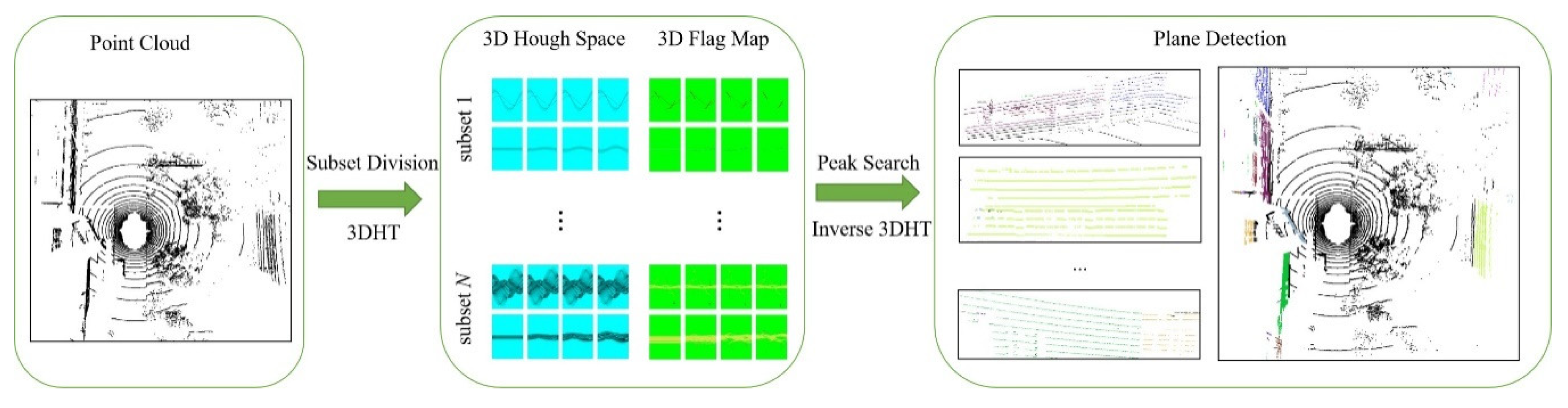
3.1. System Overview

The flowchart of our proposed fast planar detection system is shown in Figure 1. To overcome the point cloud distribution as parallel and horizontal circles in a plane surface, raw point clouds of a whole scene P are divided into individual N subsets P_m ∈ P based on the storage order. The count N of sub Hough spaces is equal to the subsets’ count of point clouds. LiDAR rotate scans the environment in a sector form for each frame so that the sensed points are stored sector by sector in horizontal orientation. This way, the sensed points in a subset P_m locate in the sector of a certain horizontal angle. After dividing global point clouds into several individual subsets, a series of Hough spaces are generated using the 3DTH algorithm. Each subset point cloud P_m generates a corresponding sub Hough space H_m, shown as the blue block in the middle part of Figure 1. Because of the random distribution and non-ideal shapes of outdoor objects, peaks representing the target plane surfaces always exist in several clusters of the valid cells in the generated Hough space. Traditional peak searching methods therefore are not applicable to simultaneously extract multiple peaks in different clusters. Thus, a 3D flag map is generated and updated using a connected component labelling algorithm for each Hough space to cluster connected cells with valid values. As shown in Figure 1, green pixels in the 3D flag map represent the invalid flag cells, and the pixels in other colors represent valid cells. The description of the 3D Hough space and 3D flag map updating method are detailed in Section 4.1.

Several cells with peak values are subsequently extracted from corresponding clusters. The coordinate values of extracted cells with peaks in a polar coordinate system of planar slides in each point subset are obtained. The separate detected planar slides of the same parameters are merged into an entire plane. To reduce the time consumption in plane detection, this study uses a parallel computing technology to modify the traditional 3DHT into the parallel 3DHT algorithm.

3.2. 3D Hough Space Generation

A planar surface in Cartesian coordinates is represented as Equation (1), where the parameters (θ, φ, r) are shown in Figure 2a. For each point, a serial of variable pairs (θ, φ, r) are sampled and registered into a 3D Hough space, as shown in Figure 2b.

$$\left(\cos \left(\theta \right)\sin \left(\phi \right),\sin \left(\theta \right)\sin \left(\phi \right),\cos \left(\phi \right),-r\right){\left(x,y,z,1\right)}^T=0$$

(1)

In the 3D Hough space generation process, the radius r_t,i,j is computed based on the horizontal angle θ_i, the vertical angle φ_j, and the LiDAR point p_t. The variables i and j are the index values of angle θ and φ, respectively, in the Hough space. Vector a_i,j is a 3 × 1 column vector forming three sine and cosine pairs, where a_i,j = [cos(θ_i)sin(φ_j), sin(θ_i)sin(φ_j), cos(φ_j)]^T, I ∈ [1, I], j ∈ [1, J]. The variable t is the index value of point p_t = [x_t, y_t, z_t], t ∈ [1, n]. The set A is comprised by vector a_i,j, which is defined as vector a_i,j ϵ A, A={a_1,1,…, a_i,j,,…, a_I,J}, i ∈ [1, I], j ∈ [1, J].

$$r_{t,i,j}=p_t{a}_{i,j}=\left[{\begin{array}{ccc}{x}_t& y_t& z\end{array}}_t\right]\left[\begin{array}{c}\cos ({\theta }_i)\sin ({\phi }_j)\\ \sin ({\theta }_i)\sin ({\phi }_j)\\ \cos ({\phi }_j)\end{array}\right]$$

(2)

In Cartesian coordinates, the subset point coordinate matrix P_m is formed by the coordinate vectors X_m, Y_m, and Z_m, which consist of a series of x, y, z point coordinates. The subset P_m is defined as P_m = [p₁, …, p_t, …p_n], t ∈ [1, n]. The variable m is the subset index, m ∈ [1, N]. R_m,i,j is the radius set that is computed by all points in the subset P_m under the angel vector a_i,j, as shown in Equation (3), defined as R_m,i,j = [r_1,i,j, …, r_t,i,j, …, r_n,i,j]. The R_m,i,j computed by a_i,j is registered into the sub Hough space H_m.

$$R_{m,i,j}=P_m{a}_{i,j}=\left[\begin{array}{ccc}{X}_m& Y_m& Z_m\end{array}\right]a_{i,j}=\left[\begin{array}{ccc}{x}_{m,1}& y_{m,1}& z_{m,1}\\ \dots & \dots & \dots \\ x_{m,t}& y_{m,t}& z_{m,t}\\ \dots & \dots & \dots \\ x_{m,n}& y_{m,n}& z_{m,n}\end{array}\right]\left[\begin{array}{c}\cos ({\theta }_i)\sin ({\phi }_j)\\ \sin ({\theta }_i)\sin ({\phi }_j)\\ \cos ({\phi }_j)\end{array}\right]$$

(3)

This way, Hough space generation is finished after all the point cloud subsets executing the 3DHT. The value in the accumulated Hough space means that the mapping point counts in the corresponding cell. The corresponding cell indices in three directions (θ, φ, r) are considered as planar surface parameters in a polar coordinate system.

3.3. Flag Map Generation

In the 3D connected component labelling algorithm, a 3D flag map L is generated as a reference to mark the high-value cells in the Hough space buffer H. The generated Hough space and its corresponding 3D flag map, where θ, φ, and r are their coordinates. The sizes in length, width, and height of both the Hough space and 3D flag map are same.

Using Equation (4), the flag map is initialized by allocating each cell with a unique label before the connected component labeling iteration process. The index pair (i, j, k) presents the cell’s location in three directions at the Hough space (θ, φ, r). The h (i, j, k) is the cell value at Hough space buffer. The equation l (i, j, k) represents the cell values of the flag map, where i, j, k is the cell index in three parameters θ, φ, and r at the flag map. When cell values h (i, j, k) in a Hough space buffer are larger than a predefined threshold γ, the corresponding values l (i, j, k) in the flag map are initialized as their unique location indices, as shown in Equation (4), where I, J, K represents the count of cells at the three dimensions θ, φ, and r. Otherwise, when cell values h (i, j, k) are less than γ, meaning not high-value valid cells in the Hough space, the corresponding values l (i, j, k) in the flag map are set as invalid. In this way, each valid cell in the flag map owns a unique value.

$$l\left(i,j,k\right)=\{\begin{array}{c}i+k\times I+j\times I\times K\\ -1\end{array}\begin{array}{c}\\ \end{array}\begin{array}{c}h\left(i,j,k\right)\ge \gamma \\ h(i,j,k)<\gamma \end{array}$$

(4)

The self-adaptive threshold value γ is computed according to Equation (5). The threshold γ is indicated based on the maximum value H_max and the average value H_aver of the Hough space. The factor λ is a constant usually located in interval [0.6, 0.8] in our experiment.

$$\gamma =H_{\max }-\lambda \ast \left(H_{\max }-H_{aver}\right)$$

(5)

After flag map initialization, a neighbour clique descriptor N_c of the cell c (i, j, k) is defined as Equation (6). All valid cells in the 3D flag map is defined as a set S. The distance between centre cell c (i, j, k) and its neighbour cell c’ (i’, j’, k’) is limited. When the distance is less than or equal to a distance threshold d, the c’ (i’, j’, k’) is considered as belonging to the descriptor N_c.

$$N_c=\left\{c^{\prime }\in S|\sqrt{{\left(i_{c’}-i_c\right)}^2+{\left(j_{c’}-j_c\right)}^2+{\left(k_{c’}-k_c\right)}^2}\le d,c\ne c’\right\}$$

(6)

If the threshold d is equal to 1, a neighborhood clique descriptor contains 6 neighboring cells (i’, j’, k’), as shown in Figure 3. In a 3D flag map updating process, a minimal value is searched out from the value l (i, j, k) of the center cell and values l (i’, j’, k’) of its neighboring cells using the descriptor.

The center cell value l (i, j, k) is subsequently updated as the searched minimum through several iterations based on Equation (7). Variable t means the iteration time in the label updating process. The values of all valid cells in the flag map are traversed using descriptors for several times until there are no values changes anymore.

$$l_{t+1}\left(c\right)=\min \left(\forall l_t\left(c^{\prime }\right)\right)\begin{array}{cc}& c^{\prime }\in N_c\end{array}$$

(7)

In this way, the cells belonging to a same connected component are updated as the same flag value. Each component containing several connected cells has a unique flag value. By matching the flag map to the Hough space, cells owing the same flag value are clustered into same clusters at the Hough space. In each cluster in the Hough space, the peak value is extracted through traversing all the cells in the cluster. The coordinates of the peak are computed as the planes’ parameters, as shown in Figure 4 in the end of the sentence.

Using Equation (1), the peaks’ coordinates (i, j, k) in the Hough space (θ, φ, r) are transformed to targeting plane parameters in a Cartesian coordinate system using Equation (1), as the inverse process.

3.4. CPU–GPU Hybrid System

To enhance the speed performance in the peak value searching process, we optimise a traditional CPU-based searching process into a CPU–GPU hybrid architecture with high-speed performance. Figure 5 presents the flowchart of our proposed plane detection system, in which CPU and GPU devices are simultaneously utilised to improve the operation efficiency. The input datasets and output results of the system are raw point clouds and estimated plane parameters, respectively. The data transmission and computation occurring in the associated work between CPU and GPU devices are explained as follows.

After dividing global point clouds into individual subsets, our proposed 3DHT algorithm is applied to each point subset to generate their corresponding 3D Hough Space in parallel. Owing to the memory size and thread count of a CPU device, point subsets are subsequently copied from the CPU to the GPU to execute sequence procedures one by one. In the GPU memory, the 3D Hough space is created with three dimensions that represent the parameters theta θ, radius r, and phi φ, as the variables in Equation (1). The resolution, representing the defined size of each cell, of the Hough space is determined by the environmental condition during the initialisation process. The points in each subset are subsequently transformed into the Hough space in parallel. When completing the transformation and statistic processes of each subset, the Hough space is updated with complete mapping information. In each thread on the GPU device, variable r is computed based on different variable pair (θ, φ) and a point coordinate. These threads are computed simultaneously, so that the 3DHT algorithm is processed in parallel.

In individual Hough space buffer, the connected component labelling algorithm is applied to cluster cells with high values into separated clusters. Several peaks are extracted from the Hough space by parallel. These peaks’ coordinates are converted to the parameter in Equation (1). All the extracted peak parameters are copied from GPU memory to CPU memory. During the plane merging process, if two planes are very similar or nearly belonging to a same plane, their plane parameters are merged together. If the distance of two peaks generated from two different subset P is less than a predefined threshold κ, the two detected planes are considered as the same one and are merged into one plane.

4. Experiments and Analysis

The experiment platform of this paper is shown in Figure 6, where a Velodyne HDL-32E sensor is used to collect LiDAR point clouds. The experiment was executed on a laptop computer with a 2.21 GHz Inter^® Core™ (Santa Clara, CA USA) i7-8750 CPU @2.20 GHz, GeForce GTX 1070 Ti graphics card, and 16 GB RAM in Windows 10 operation system.

4.1. Three-Dimensional Hough Space and Flag Map Performance

The generated 3D Hough space buffer is shown in Figure 7, where theta θ, radius r, and phi φ are three coordinate axes. The cross sections perpendicular to the φ axis are displayed sequentially as the value φ increases.

Figure 8a,b show the Hough space generated by all point clouds and a fraction of point clouds, respectively. Figure 8a illustrates images of θ-r cross sections under different φ values in the Hough space generated by all point clouds. The entire point clouds are massive and inhomogeneous, causing a distribution with high complexity in the Hough space, as shown in Figure 8a. The peak values generated in the Hough space buffer therefore are difficult to be extracted, meaning that the accuracy of planar reduces. Figure 8b shows the Hough space generated by a fraction of points after being divided. As presented in the figure, when the number of points after division is rather small and the coverage area is also relatively small, the generated Hough space is clear and efficient, where the peak values can be easily extracted and precisely represent the planar surfaces in a fraction area. In the Hough space, the ranges of the variables θ, φ, and r was between 0° to 360°, 0° to 180°, and 0 to 100 m, respectively. Accordingly, the resolutions were 1°, 5 dm, and 5°, respectively. The coordinates (θ, φ, r) of cells with peak values were recorded as planar slide parameters in the Hough space. Because of the limited memory of GPU devices, the resolution of variable θ was set higher than that of axis φ to ensure that the detection of planes in the vertical direction shows a higher accuracy.

Figure 8c,d illustrates the 3D flag map generated from the Hough space buffer in Figure 8a,b, where different cell clusters are rendered in different colors. As shown in Figure 8c, due to the horizontal linear distribution of LiDAR point clouds, a large number of valid cells are clustered into a cluster with a strip shape in the middle of the flag map. The peak searching in such cluster was against our purpose of performing clustering before peak searching, for its undiminished complexity and unincreased accuracy. The clusters in the flag map generated by a fraction of points, however, were concentrated in several separated parts. The peak of each cluster is searched with a higher accuracy, as shown in Figure 8d. Therefore, the Hough space generated by a fraction of points was more applicable for subsequent peak extraction than that generated by all points.

4.2. Multiple Fraction Integration

Compared with dense point cloud data, which were evenly distributed and possess good point features, an LiDAR point cloud tended to be sparse and inhomogeneous, and valid point features were hard to extract. Considering that the LiDAR acquired environment data along the scan line, the point cloud had a higher density on horizontal scan lines. However, in the vertical direction, the spacing between the horizontal scan lines increased as the distance from the scanning centre rose, rendering point clouds in the vertical direction sparse and unevenly distributed. Therefore, the Hough transform method could be extensively used in plane detection from dense point clouds and in obtaining accurate detection results. However, given that the points on the horizontal scan lines were superior in numbers in sparse LiDAR point clouds, imprecise results, such as horizontal plane detection (Figure 9), would frequently emerge and lead to adverse effects on the detection of vertical walls. Therefore, the traditional Hough transform method was not applicable to plane detection of the LiDAR point cloud.

Thus, the fraction-to-fraction Hough Transform method was employed in this study to detect plane surfaces in the environment, rather than the Hough Transform directly applied to obtain point clouds in the entire area. The collected point clouds were firstly divided into several fractions in different regions with a defined number of points. Then, the proposed parallel 3DHT method was applied to one fraction in a single frame until all fractions have been processed. After all the Hough space buffers were established, peak cells in different buffers were extracted out using a 3D connected component labelling algorithm. The parameters of the multiple detected planar slides would be obtained, through which our detection targets, including the vertical walls in the sensed environment, could be merged and displayed. To merge the planar slides detected in different fractions, which belong to a same plane surface, a threshold κ was utilized to judge the parameter differences between several sub planes. In our application, the threshold κ was set as 3. If the κ is high, some non-coplanar planes were merged into one plane. If the κ was small, some coplanar planes couldn’t be merged. Until all the sub planes’ parameters were measured by the threshold, the merge process was finished with the detection result of target planes.

4.3. Parallel 3DHT Performance

As illustrated in Section 3.2, the Hough space is generated by computing each radius r according to each parameter pair (θ, φ). In a traditional 3DHT algorithm, the computational complexity of generating a Hough space with number N points reaching O (I × J × N), where I and J represent the count of θ and φ values. The time consumption for the generation process increases with the resolutions.

In estimating the operating efficiency of our proposed system, we utilized the frame per second (fps) as the evaluation method to compare the Hough space generating time using the entire point clouds and fractions of point clouds in approximately 90 different frames shown in Figure 10. Figure 10 illustrates the recorded fps of the generated Hough space in different resolutions when all of the point clouds and fractions are used.

As shown in Figure 10a,b, a higher resolution corresponds to a lower fps. As the resolution value increases, the fluctuation of the fps curves becomes more evident. Figure 10a illustrates the recorded fps in generating the Hough space with all of the point clouds in different resolutions at approximately 100 different frames. When the resolution reaches 4.0, the overall values of fps are the highest among the compared datasets, fluctuating between 80 and 100. Before the 45th frame, the fps values in resolution 4.0, whose changing trade remains steady, fluctuate at approximately 80. After the 45th frame, the changing trade becomes relatively volatile, where several recorded values reach or exceed 100 fps. Figure 10b shows the condition when generating Hough space with multiple fractions. When the resolution is 10.0, the fps values, fluctuating smoothly between 25 and 30 fps, are higher than the fps values whose resolution is lower than 10.0. By comparing Figure 10a,b, the fps curve when using all of the points to generate Hough space is much lower and unstable than that which uses the proposed fraction-to-fraction method when the resolution values are equal.

Table 1. Plane detecting the fps comparison.

Type and Resolution	Fps
CPU-based RANSAC	0.1999
GPU-based RANSAC	4.6109
GPU-based Hough transform (resolution 1.0, single frame)	3.1167
GPU-based Hough transform (resolution 2.0, single frame)	12.3693
GPU-based Hough transform (resolution 3.0, single frame)	27.8686
GPU-based Hough transform (resolution 5.0, multiple frames)	1.8678
GPU-based Hough transform (resolution 10.0, multiple frames)	8.8794

presents the fps of the plane detection that uses the RANSAC and Hough transform based on CPU and GPU computing. As presented on the table, the efficiency of RANSAC based on parallel computing is remarkably improved compared with the traditional RANSAC. In our proposed parallel 3DHT algorithm, when the resolution value is approximately 10.0, the multi-frame average fps exceeds that of the RANSAC algorithm. When the resolution is higher, the fps of a single frame also remarkably surpasses RANSAC, as shown in resolutions 2.0 and 3.0. Therefore, unlike the GPU-based RANSAC, our proposed method can significantly improve the computing speed in plane detection when an appropriate resolution value is adopted.

The speed efficiency of the plane surface detection that uses our developed parallel 3DHT algorithm has a noticeable improvement when compared with our previous work through the RANSAC algorithm [27] and CUDA-based RANSAC [29].

4.4. Multiple Fraction Integration

Figure 11 demonstrate plane detecting results by using our proposed fraction-to-fraction parallel 3DHT. The plane detection results in Figure 11a,c,d are more accurate than those featured in Figure 11b. As illustrated in Figure 11d, only one noticeable plane is presented in the scene, ensuring that it is detected precisely. However, because of the complex building outline in Figure 11a, the plane recognizing results were not satisfied, where several small planes were ignored. Because the sizeable parts of the raw point clouds are located on ground surfaces, a ground point filtering is an essential pre-process step before transforming 3D points into the Hough space. The random and stochastic occurrence of 3D objects in outdoor environments causes an irregular numerical distribution in the accumulated Hough space. Thus, the traditional Hough transform directly applied to the entire point clouds will be easily disturbed, thereby causing an inaccurate detection result.

5. Conclusions

This study developed a fraction-to-fraction 3DHT algorithm to detect the plane surface from an LiDAR point cloud. Considering the importance of time efficiency in our plane detecting application, this paper adopted GPU-based parallel computing technology so that the average speed performance of the CPU–GPU hybrid plane detection method is around 12.37~27.87 fps in a single frame. Besides, the accurate performance of the plane detection result in outdoor environment is higher than that without using our proposed fraction-to-fraction parallel 3DHT algorithm. Even though our testing datasets are quite complex, with lots of irregular outdoor objects, most planar surface were detected efficiently.

References

1. Asvadi, A.; Premebida, C.; Peixoto, P.; Nunes, U. 3D Lidar-based static and moving obstacle detection in driving environments: An approach based on voxels and multi-region ground planes. Robot. Auton. Syst. 2016, 83, 299–311. [Google Scholar] [CrossRef]
2. Ramiya, A.M.; Nidamanuri, R.R.; Krishnan, R. Segmentation based building detection approach from LiDAR point cloud. Egypt. J. Remote Sens. Space Sci. 2017, 20, 71–77. [Google Scholar] [CrossRef] [Green Version]
3. Kim, P.; Chen, J.; Cho, Y.K. SLAM-Driven robotic mapping and registration of 3D point clouds. Autom. Constr. 2018, 89, 38–48. [Google Scholar] [CrossRef]
4. Awrangjeb, M.; Zhang, C.; Fraser, C.S. Automatic extraction of building roofs using LIDAR data and multispectral imagery. ISPRS J. Photogramm. 2013, 83, 1–18. [Google Scholar] [CrossRef] [Green Version]
5. Wang, H.; Wang, B.; Liu, B.; Meng, X.; Yang, G. Pedestrian recognition and tracking using 3D LiDAR for autonomous vehicle. Robot. Auton. Syst. 2017, 88, 71–78. [Google Scholar] [CrossRef]
6. Limberger, F.A.; Oliveira, M.M. Real-Time detection of planar regions in unorganized point clouds. Pattern Recognit. 2015, 48, 2043–2053. [Google Scholar] [CrossRef] [Green Version]
7. Sayed, E.E.; Kader, R.F.A.; Nashaat, H.; Marie, M. Plane detection in 3D point cloud using octree-balanced density down-sampling and iterative adaptive plane extraction. IET Image Process. 2018, 12, 1595–1605. [Google Scholar] [CrossRef] [Green Version]
8. Czerniawski, T.; Nahangi, M.; Walbridge, S.; Haas, C. Automated removal of planar clutter from 3D point clouds for improving industrial object recognition. In Proceedings of the 33rd International Symposium on Automation and Robotics in Construction (ISARC 2016), Auburn, AL, USA, 18–21 July 2016. [Google Scholar]
9. Feng, C.; Taguchi, Y.; Kamat, V.R. Fast plane extraction in organized point clouds using agglomerative hierarchical clustering. In Proceedings of the IEEE International Conference on Robotics & Automation (ICRA), Hong Kong, China, 31 May–7 June 2014. [Google Scholar]
10. Hulik, R.; Spanel, M.; Smrz, P.; Materna, Z. Continuous plane detection in point-cloud data based on 3D Hough Transform. J. Vis. Commun. Image 2014, 25, 86–97. [Google Scholar] [CrossRef]
11. Liang, Y.B.; Zhan, Q.M.; Che, E.Z.; Chen, M.-W.; Zhang, D.-L. Automatic registration of terrestrial laser scanning data using precisely located artificial planar targets. IEEE Geosci. Remote Sens. 2014, 11, 69–73. [Google Scholar] [CrossRef]
12. Abdullah, S.; Awrangjeb, M.; Lu, G. LiDAR segmentation using suitable seed points for 3D building extraction. Int. Arch. Photogramm. Remote Sens. Spat. Inf. Sci. 2014, 3, 1–8. [Google Scholar] [CrossRef]
13. Deschaud, J.; Goulette, F. A Fast and accurate plane detection algorithm for large noisy point clouds using filtered normals and voxel growing. J. Vis. Commun. Image Represent. 2014, 25, 86–97. [Google Scholar]
14. Vo, A.V.; Linh, T.; Laefer, D.F.; Bertolotto, M. Octree-Based region growing for point cloud segmentation. ISPRS J. Photogramm. 2015, 104, 88–100. [Google Scholar] [CrossRef]
15. Whelan, T.; Ma, L.; Bondarev, E.; de With, P.N.H.; McDonald, J. Incremental and batch planar simplification of dense point cloud maps. Robot. Auton. Syst. 2015, 69, 3–14. [Google Scholar] [CrossRef] [Green Version]
16. Nurunnabi, A.; Belton, D.; West, G. Robust statistical approaches for local planar surface fitting in 3D laser scanning data. ISPRS J. Photogramm. 2014, 96, 106–122. [Google Scholar] [CrossRef] [Green Version]
17. Yeon, S.; Jun, C.; Choi, H.; Kang, J.; Yun, Y.; Lett Doh, N. Robust-PCA-based hierarchical plane extraction for application to geometric 3D indoor mapping. Ind. Robot. 2014, 41, 203–212. [Google Scholar] [CrossRef]
18. Galloa, O.; Manduchia, R.; Rafiib, A. CC-RANSAC: Fitting planes in the presence of multiple surfaces in range data. Pattern Recogn. Lett. 2011, 32, 403–410. [Google Scholar] [CrossRef] [Green Version]
19. Qian, X.; Ye, C. NCC-RANSAC: A fast plane extraction method for 3-D range data segmentation. IEEE Trans. Cybern. 2014, 44, 2771–2783. [Google Scholar] [CrossRef]
20. Yue, W.; Lu, J.; Zhou, W.; Miao, Y. A new plane segmentation method of point cloud based on mean shift and RANSAC. Chin. Control Decis. Conf. 2018, 1658–1663. [Google Scholar] [CrossRef]
21. Li, L.; Yang, F.; Zhu, H. An improved RANSAC for 3D point cloud plane segmentation based on normal distribution transformation cells. Remote Sens. 2017, 9, 5. [Google Scholar] [CrossRef] [Green Version]
22. Alehdaghi, M.; Esfahani, M.A.; Harati, A. Parallel RANSAC: Speeding up plane extraction in RGBD image sequences using GPU. In Proceedings of the 5th International Conference on Computer and Knowledge Engineering (ICCKE), Zurich, Switzerland, 29–30 October 2015; pp. 295–300. [Google Scholar]
23. Vera, E.; Lucio, D.; Fernandes, L.A.F.; Velho, L. Hough transform for real-time plane detection in depth images. Pattern Recogn Lett. 2018, 103, 8–15. [Google Scholar] [CrossRef]
24. Jeltsch, M.; Dalitz, C.; Fröhlich, R.P. Hough parameter space regularisation for line detection in 3D. In Proceedings of the International Conference on Computer Vision Theory and Applications (VISAPP), Rome, Italy, 17 October 2016; pp. 345–352. [Google Scholar]
25. Maltezos, E.; Ioannidis, C. Plane detection of polyhedral cultural heritage monuments: The case of tower of winds in Athens. J. Archaeol. Sci. Rep. 2018, 19, 562–574. [Google Scholar] [CrossRef]
26. Marriott, R.T.; Pashevich, A.; Horaud, R. Plane-Extraction from depth-data using a Gaussian mixture regression model. Pattern Recogn. Lett. 2018, 110, 44–50. [Google Scholar] [CrossRef] [Green Version]
27. Lan, J.; Tian, Y.; Song, W.; Fong, S.; Su, Z. A fast planner detection method in LiDAR point clouds using GPU-based RANSAC. In Proceedings of the KDD 2018 Workshop on Knowledge Discovery and User Modelling for Smart Cities, London, UK, 20 August 2018; pp. 8–35. [Google Scholar]
28. Song, W.; Liu, L.; Tian, Y.; Sun, G.; Fong, S.; Cho, G. A 3D localisation method in indoor environments for virtual reality applications. Hum. Centric Comput. Inf. Sci. 2017, 7, 39. [Google Scholar] [CrossRef] [Green Version]
29. Vega-Rodríguez, M.A.; Pavón, N.; Ferruz, J. A Comparative study of parallel RANSAC implementations in 3D space. Int. J. Parallel Program. 2014, 43, 703–720. [Google Scholar]
Figure 1. Flowchart of the fast planar detection system.
Applsci 10 01744 g001
Figure 2. The graphical illustration of a Cartesian coordinate and a 3D Hough space. (a) The Cartesian coordinate. (b) The Hough space.
Applsci 10 01744 g002
Figure 3. Three-dimensional flag map and descriptor.
Applsci 10 01744 g003
Figure 4. Peaks searched from a 3D flag map.
Applsci 10 01744 g004
Figure 5. CPU–GPU hybrid architecture of fast planar detection system.
Applsci 10 01744 g005
Figure 6. Unmanned vehicle platform with light detection and ranging (LiDAR).
Applsci 10 01744 g006
Figure 7. Display order of a 3D Hough space buffer.
Applsci 10 01744 g007
Figure 8. Hough space and flag maps generated by all point clouds and a fraction of point clouds. (a) The Hough space generated by all point clouds in a frame. (b) The Hough space generated by a fraction of the point clouds in a frame. (c) The flag map generated by all point clouds using a connected component labelling algorithm. (d) The flag map generated by a fraction point cloud using a connected component labelling algorithm.
Applsci 10 01744 g008
Figure 9. Error in the plane detection result of the parallel three-dimensional Hough transform (3DHT).
Applsci 10 01744 g009
Figure 10. Speed performance and time consumption in generating Hough space. (a) The Hough space generating time using all of the point clouds. (b) The Hough space generating time using multiple fractions.
Applsci 10 01744 g010
Figure 11. Plane detection results in different types of outdoor environments. (a) dataset 1; (b) dataset 2; (c) dataset 3; (d) dataset 4.
Applsci 10 01744 g011aApplsci 10 01744 g011b