Abstract
The present paper deals with the problem of modeling liquid slosh occurring in the packaging process of containers filled with liquid. Sloshing effects are induced by one-dimensional intermittent motions and are undesired due to the necessity of quality control processes, such as weighing. Therefore, motion optimizations are often applied with the intention to minimize the residual vibrations. Valid process models are required to do so. The aim of this paper is to derive models for describing the liquid slosh behavior for different motions and for common practical circumstances, e.g., different container geometries as well as machine operating speeds, and to state the model’s limits of use. Known model approaches are discussed, and their assumptions are reviewed experimentally. This leads to a set of limited ranges of operating speeds in which the applied models’ assumptions are valid. The models are derived for these sets from experimental data, and a comparison is executed that enables the determination of the models’ validity concerning their operating speed dependency. Finally, the validity of the derived models is investigated by comparing their predictive efficiency of describing the vibration for different motion profiles.
1. Introduction
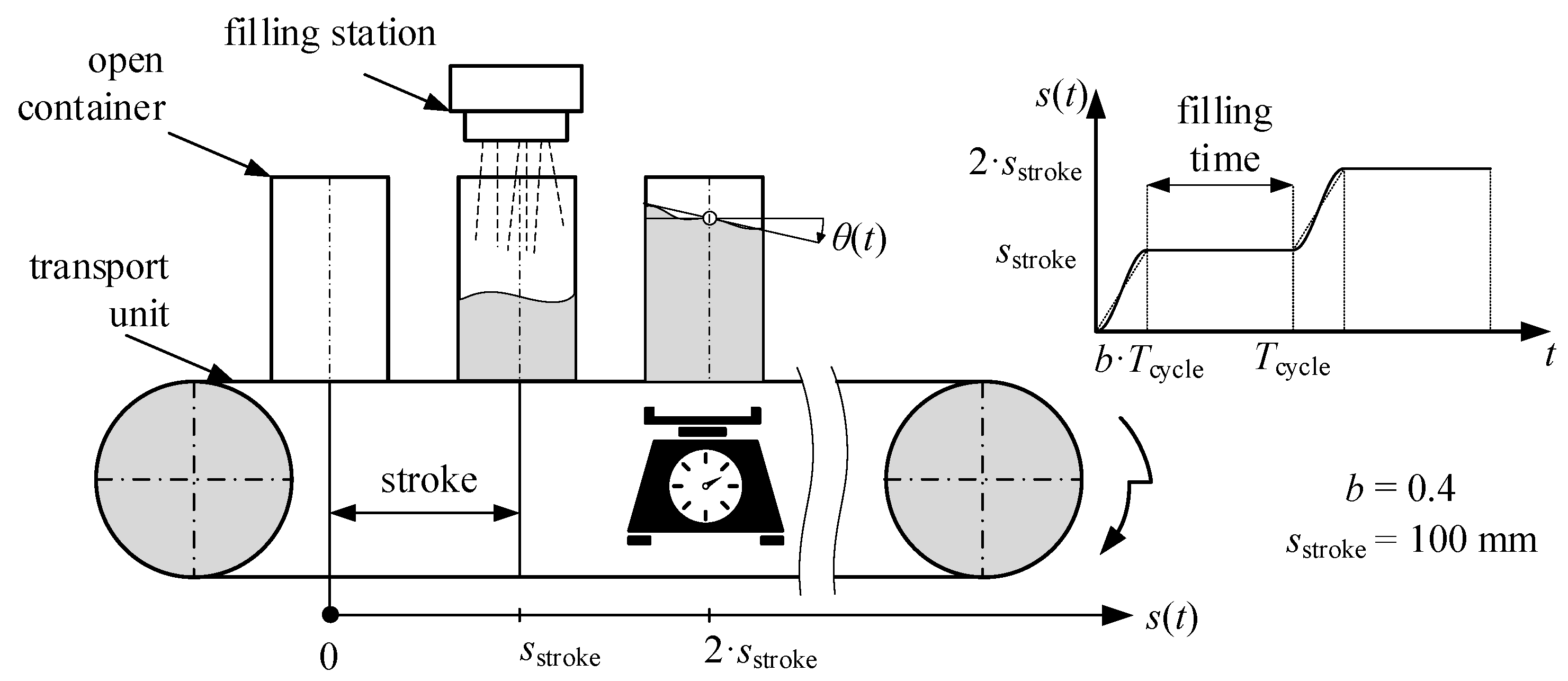
The investigation of liquid slosh dates back to the 1960s and was initially motivated by aerospace research [1,2]. Later on, more practical use cases of this phenomena were investigated [3]. One practical application of the underlying physical problem occurs in packaging machines producing beverages, displayed in Figure 1. Due to high requirements in the production process of daily needs such as food and beverages, packaging machines are intended to produce at maximum productivity. Often, neither the mechanical nor the mechatronical components limit the machine’s operating speed and hence the productivity. In fact, the behavior of the materials to be processed limits the maximum achievable operating speed [4]. For instance, residual vibration induced by the applied intermittent motion profile is to be avoided, e.g., due to necessary quality control processes. Hence, the motion optimization of the conveying motion is a powerful method for minimizing the residual vibration. The optimization of the motion profile is a suitable possibility for the given problem, but it is less widespread in industrial practice [5]. Nevertheless, a valid model that predicts the sloshing behavior depending on a motion profile is needed for motion optimization.
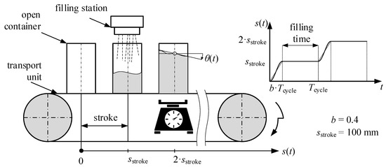
Figure 1.
Principle of a filling unit applied in packaging machines. Empty, open containers are conveyed by a linear transport unit that realizes a rise-to-dwell-motion. After filling in the fluid, the filled container is conveyed to a weighing station, where the bottled fluid’s mass is controlled. For doing this, minimum residual vibration of the fluid’s surface is essential. The exemplary conveying motion consists of a motion time with length and a dwell phase of length . Here, a stroke of 100 mm as well as a ratio of motion time to cycle time of are assumed.
Model approaches can principally be subdivided into two main classes, namely descriptive models and explanatory models [6]. In the case of modeling liquid slosh, explanatory approaches use the Navier–Stokes equations for describing the liquid–container interaction as a continuum problem. Therefore, material parameters, such as viscosity and density, are considered as distributed parameters. Such a general approach leads to a system of partial differential equations [7,8,9]. This system of equations is not solvable analytically, wherefore numerical solution techniques such as the finite difference method or the finite volume method have to be applied [10,11,12,13]. Models with distributed parameters can be used for motion optimization as shown in [14,15]. Such solutions are associated with enormous calculation times, although the presented solutions already represent an approximation of the partial differential equation system. Another possibility is the modeling with concentrated parameters and physical substitution models such as the pendulum model, also discussed in [7]. This approach leads to an ordinary differential equation of order two, which can be easily considered in common motion optimization algorithms in an efficient way [16,17].
A new aspect of research in the field of model-based motion optimization is the operating-speed-dependent motion profiles that are discussed in [18,19]. Applying this approach to the motion optimization for liquid slosh, the previous modeling work has to be re-investigated and discussed regarding their operating-speed-dependent usability. Hence, this paper aims to answer two main questions regarding the modeling of liquid slosh with the purpose for using it in operating-speed-dependent motion optimizations:
- Are there limitations of the substitution mechanical slosh models concerning the applicable operating speed?
- If such limitations can be stated, are the derived models applicable for the whole derived range of operating speeds and at what accuracy?
For taking into account the special case of liquid slosh occurring in packaging machines, the following limitations are assumed: only one-dimensional motions and transient excitations are considered due to considering only one machine cycle—in contrast to investigations concerning periodic behavior [20]. Thus, there will be no discussion of resonances and magnification functions, since steady-state behavior must be therefore present.
2. Materials and Methods
2.1. Test Station and Experimental Design for Investigating Liquid Slosh
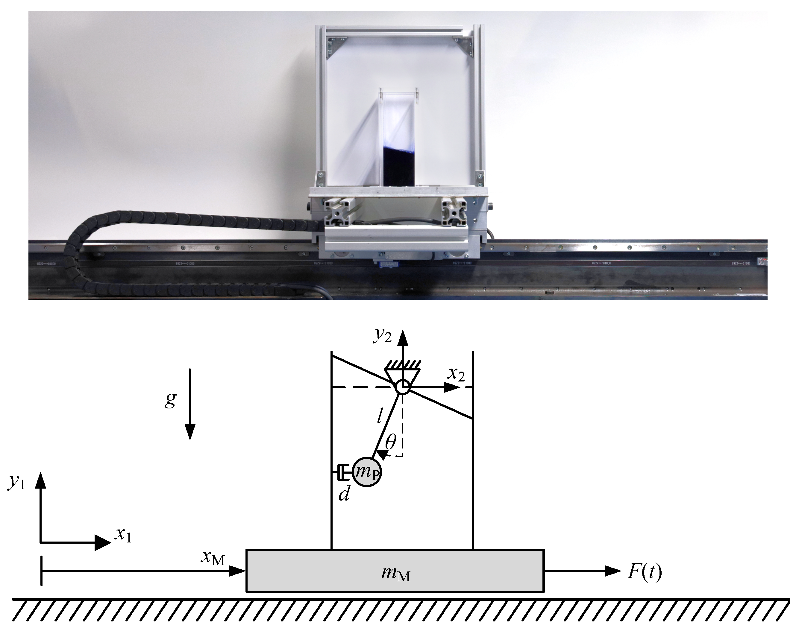
To investigate the liquid slosh behavior, a test station shown in Figure 2 was build. The station consists of a direct linear drive on which different containers can be conveyed with any desired motion profile. To observe the fluid’s behavior, a high-speed camera is coupled to the mechanical setup, whereas the camera is triggered by the motion control system. Hence, the captured frames can be synchronized with the applied motion profile, which simplifies the evaluation. In addition to that, the applied frame rate (FR) is automatically determined by the observed operating speed n. Hence, all experiments supply the same amount of frames for further investigation, independently from the applied operating speed. The specifications of the used hardware are displayed in Table 1.
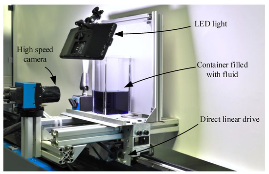
Figure 2.
Experimental setup to investigate the linear transport unit’s motion’s influence on the liquid slosh behavior for different container geometries. The different containers are clamped into a mechanical socket that is coupled to a linear direct drive. Additionally, a high speed camera and LED lighting are fixed to the mechanical setup to observe the fluid’s surface.

Table 1.
Specifications of used hardware elements in the test station.
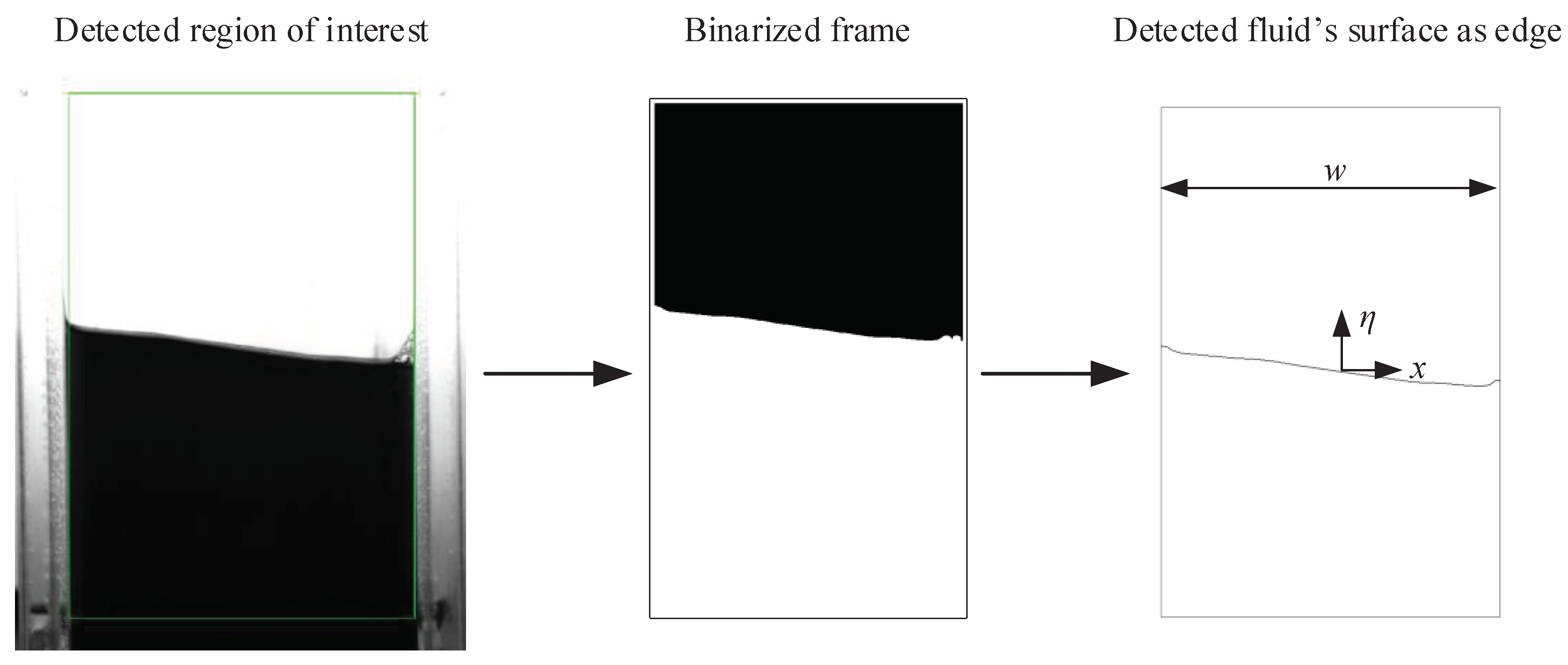
The captured high speed frames are evaluated automatically by detecting the region of interest, binarizing the frame, and finally detecting the fluid’s surface with the Canny algorithm [21] (see Figure 3).
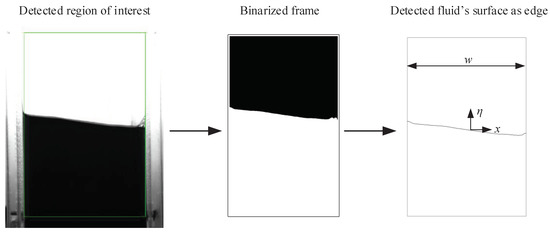
Figure 3.
Steps in detecting the fluid’s surface edge for the container’s width w: first, the region of interest is detected; second, the frame is binarized by setting a threshold value; third, the edge is detected by the Canny algorithm. The -values of the edge are saved.
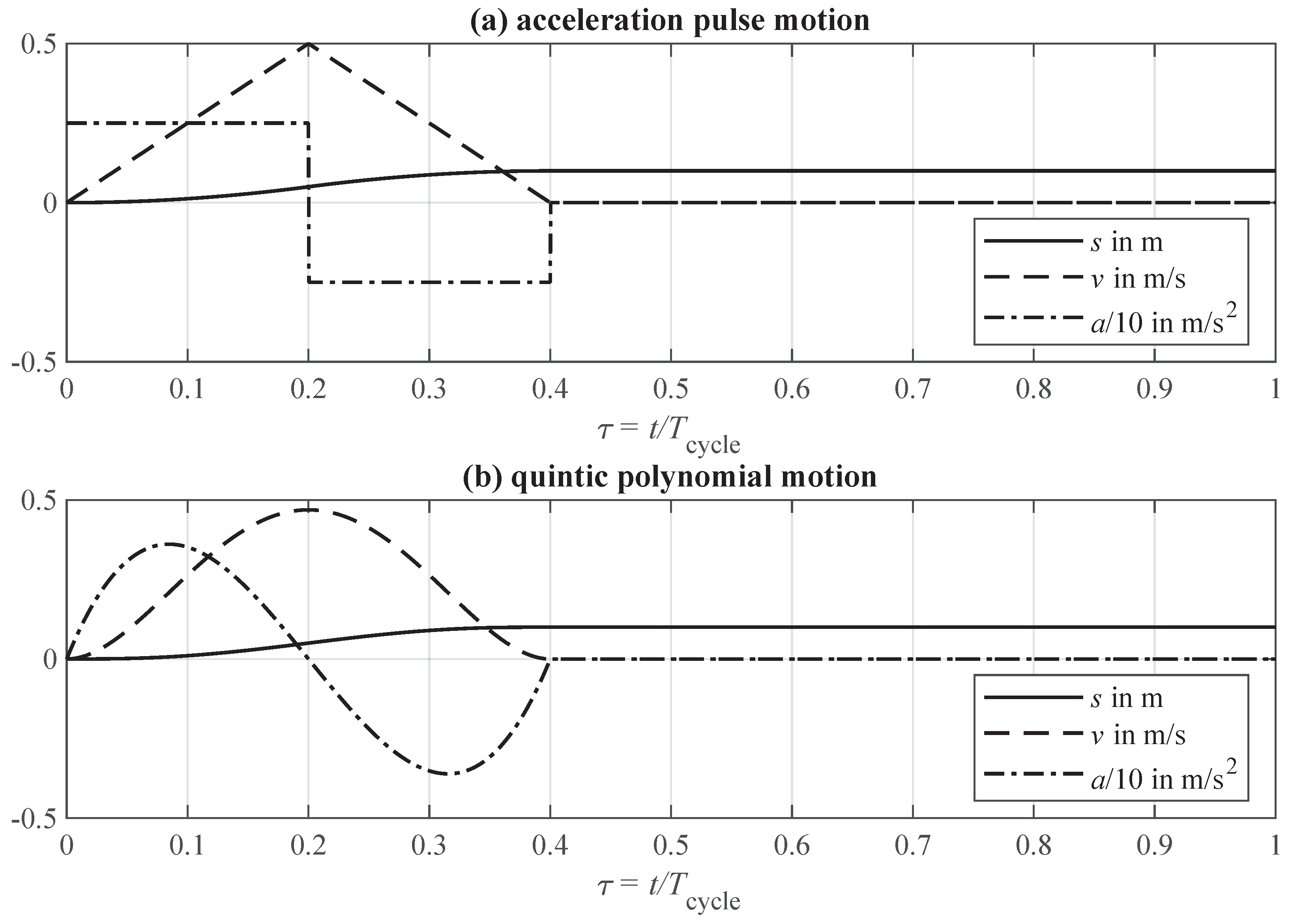
To cover a wide range of practical conditions, the experiments are carried out with six container geometries at two different motion profiles and 17 different operating speeds. The geometries differ in their width w. The exact specifications are depicted in Table 2. The stroke, velocity, and acceleration trajectories of the used motion profiles are displayed in Figure 4. Due to the high water content in everyday beverages, water is taken as the fluid to be examined.

Table 2.
Specification of experimental design for creating parameter identification and validation data.
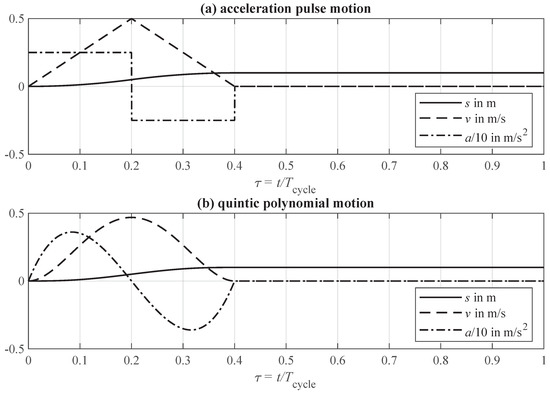
Figure 4.
Applied motion profiles calculated for a cycle time of s, displayed over the normalized time : (a) acceleration pulse motion is used for parameter identification, and (b) polynomial motion is used for generating validation measurements.
For creating the parameter identification data, all six geometries are conveyed with the acceleration pulse motion at 17 different operating speeds, whereas every experiment is repeated 10 times, represented by the constant . Hence, an amount of 1020 experiments is to be carried out and evaluated. The validation data is generated by applying the quintic polynomial motion profile, whereas each experiment is repeated five times (). Therefore, an amount of 510 experiments is to be conducted and evaluated for creating the validation data. The idea behind this strategy is that different system inputs are used for parameter identification and validation.
2.2. Modeling Liquid Slosh
In order to be able to use the model to be created for motion optimization, as few degrees of freedom as possible should be used in order to avoid unnecessary computing time. Therefore, the already mentioned mechanical pendulum model is investigated in this paper. The real system, shown in Figure 5, can be abstracted to a model consisting of a horizontally movable mass displaying the linear drive and an attached damped pendulum representing the fluid’s surface displacement with length l, mass , and damping constant d. For describing the system’s dynamic behavior, two generalized coordinates, namely as well as , are introduced, which are summarized in the vector . The system is controlled by the time-depending force affecting the mass . In contrast to [16], the model equations are motivated with respect to the applied drive.
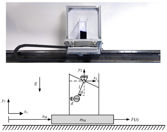
Figure 5.
Mechanical motivation for model building due to abstracting the real process. The direct linear drive is described by a force actuated mass on which a damped pendulum with length l, mass , and damping coefficient d is mounted, which describes the fluid’s surface.
According to [22], the Lagrange formalism is used for determining the equations of motion for the abstracted system. The kinetic energy T, the potential energy U of the system, and the dissipation energy D due to the damper element affecting on the pendulum are given by
Subsequently, the equations of motion can be derived with the actuating force from evaluating
This leads to a system of two nonlinear differential equations:
Considering the real system, the actuating force is caused due to a direct linear drive, which is driven by a cascade control loop with a very high dynamic stiffness. Furthermore, the drive’s mass is essentially greater than the pendulum’s mass. These two statements lead to the simplification , from which
results and, hence, the dynamical behavior of the system can be solely described with Equation (6).
Furthermore, the drive’s acceleration is redefined as the motion’s profile acceleration a. As a last step, the equation is linearized by assuming and , which leads to
Introducing the undamped angular frequency and the damping ratio , Equation (8) finally results in the model equation :
This equation describes a driven harmonic oscillator and is an ordinary differential equation of order two with two free parameters, which can be used for modeling the real system’s behavior by parameter optimization. The special feature of this equation is that the factor of the external motion profile’s acceleration results from the undamped natural frequency and the acceleration due to gravity.
A generalization of this model approach is the driven harmonic oscillator of order two with three free parameters:
In [23], it is asserted that the additional parameter p leads to a higher accuracy in depicting the real system’s behavior. This assumption is also claimed in [24] and will be experimentally investigated here. The model equations and can be solved numerically for a given set of parameters and a system input with the method of Runge–Kutta [25].
2.3. Evaluating the Model’s Assumptions
The main assumption of the derivated model above is the approximation of the fluid’s surface as a straight line. In a first step, this assumption has to be investigated, because in reality the fluid surface has a characteristic waveform. For doing so, for each geometry , operating speed , repetition k, and captured frame j corresponding to a discrete time value , an approximation in the form of a line of the measured fluid’s surface has to be derived. Therefore, the measured fluid’s surface is approximated as a linear function with time-dependent slope . This slope has to be determined as part of a parameter identification. Thus, the residuals between the measured surface edge in the discrete form and the approximated line in the discrete form surface are quadratically summed:
The value that minimizes this sum of residuals is the value to be identified:
The gradient-based algorithm of Levenberg–Marquardt [26] is applied for performing the optimization, due to the convexity of the problem. Hence, short calculation times can be achieved, which are not realizable with global optimization strategies. In Figure 6, an exemplarily sketch of a surface with an approximated line is shown, whereas the difference is displayed over the horizontal coordinate x.

Figure 6.
Results of investigating the linearity of the detected fluid surface.
The remaining residuals are a measure for the approximation’s goodness and are therefore used to score the goodness of line approximation over all discrete time points. Due to the effect of in-phase interception discussed in [19], cancellation of residual vibration may occur at some operating speeds of the motion profile. To enable comparability, the dwell phase is not considered evaluating the goodness of line approximation, which is why only the captured frames of the motion phase are considered:
Due to the repetitions of the experiments, the mean values as well as the corresponding standard deviations are examined to compare the obtained results [27]:
Setting a tolerable value for of 0.5 mm, this evaluation allows the determination of a maximum operating speed up to which the assumption of a fluid’s surface as a straight line is valid. This enables the answering of the first formulated question in the introduction.
2.4. Determining the Model Parameters and Evaluating the Model’s Goodness
For answering the second formulated question, it is to be examined whether the simulated values from the model approaches and are reproducing the approximated values of within the ascertained range of operating speeds in a suitable way. Therefore, two approaches are investigated.
First, for each operating speed and geometry , and models are examined by solving a least-squares problem, which considers all repetitions at once. Thereby, the least-square-optimization problem is solved with the Levenberg–Marquardt algorithm again. For calculating the objective function to be minimized, possible parameter candidates as well as the motion’s acceleration profile are inserted into the model equations. The resulting differential equations are solved numerically using the Runge–Kutta method in order to finally calculate the residuals between the measured and simulated values of .
Hence, a set of models are build to describe the measured behavior for its valid range of operating speeds. This strategy should be named the Single-Operating-Speed Model (SOSM). Second, for each geometry and all valid operating speeds, the models , and are examined in the same way considering all repetitions at once. Hence, for one geometry, only one model for approach and one for approach are derived. This strategy should be named the Multiple-Operating-Speed Model (MOSM).
Finally, the goodness of these different strategies and model approaches has to be examined. Therefore, the standard error of estimate () is calculated by
This value is a measure of how much the simulated value of differs on average from all approximated values of that result from the measurements. This allows the comparison of the two model approaches and as well as the two strategies SOSM and MOSM in the correspondent valid range of operating speeds. Finally, it must be checked whether the identified models can make a meaningful statement regarding the process-relevant residual sloshing behavior. First of all, an appropriate quality criterion is necessary. One possibility is the effective value of the fluid surface during the dwell phase, whose definition generally has the following form:
Due to the discretization of all treated quantities, the integrals are calculated numerically using the trapezoidal method. The investigation of this compacted size has the advantage that it can be applied to the actually measured edge courses of the fluid as well as to the approximated straight line and the simulated courses resulting from applying the mechanical model. Thus, this parameter is universally applicable and enables an evaluation of the process success, especially with regard to the investigation of the success of optimal trajectories. Furthermore, it is possible to compare the difference between real edge progression, straight line approximation, and model prediction. Therefore, measures for these differences can be considered by the following approach:
In order to describe the mean difference between the measured fluid’s edge and the approximated straight line, and the approach for describing the mean difference between the measured fluid’s edge and the simulated model response is as follows:
3. Results
3.1. Determining the Validity of the Model’s Assumptions
Evaluating Equation (13) for all 1020 parameter identification experiments led to the results displayed in Figure 7. For all six investigated geometries, the mean errors of the fluid’s line approximation rise with the operating speed n. Furthermore, the corresponding standard deviations also rise with the operating speed. Observing the six different graphs, it is noticeable that every single graph can be divided into two different ranges of operating speeds. At first, an almost horizontal course can be noticed, followed by a range of a strongly rising course. The defined limit value for of 0.5 mm forms the boundary between these two ranges and thus leads to the sought maximum operating speed for every chosen geometry. The maximum operating speeds are stated in Figure 7 for each geometry and differ from one another. It can be noted that the container’s width and the maximum operating speed are inversely proportional to each other.
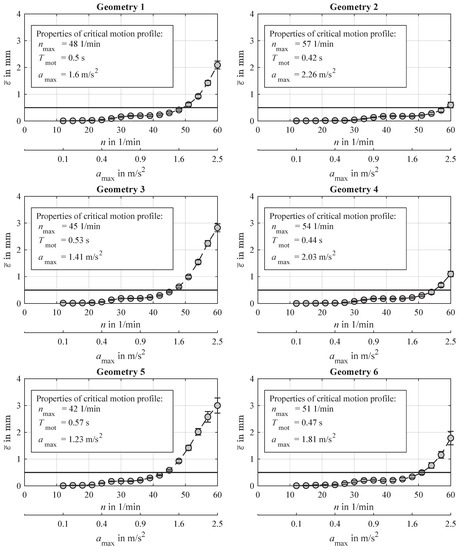
Figure 7.
Mean errors of fluid’s surface line approximations for different geometries and operating speeds as well as the correspondent standard deviations. Assuming a tolerable error of mm, a maximum operating speed is derivable. Up to this operating speed, the considered fluid’s surface motion can be described as a line, and thus can be used for the pendulum modeling.
3.2. Determining the Model’s Parameters and Their Goodness
Knowing the maximum operating speeds for all investigated geometries for which assuming the fluid surface as a straight line is valid, the discussed model approaches are derived, and the related values are calculated as a measure for the model’s goodness. Therefore, for each geometry and a valid operating speed, an SOSM approach is calculated. This leads to two models, each for one operating speed, with two and three parameters, respectively. Furthermore, for each geometry, an MOSM approach is calculated considering model equations and , resulting overall in two models with two and three parameters, respectively.
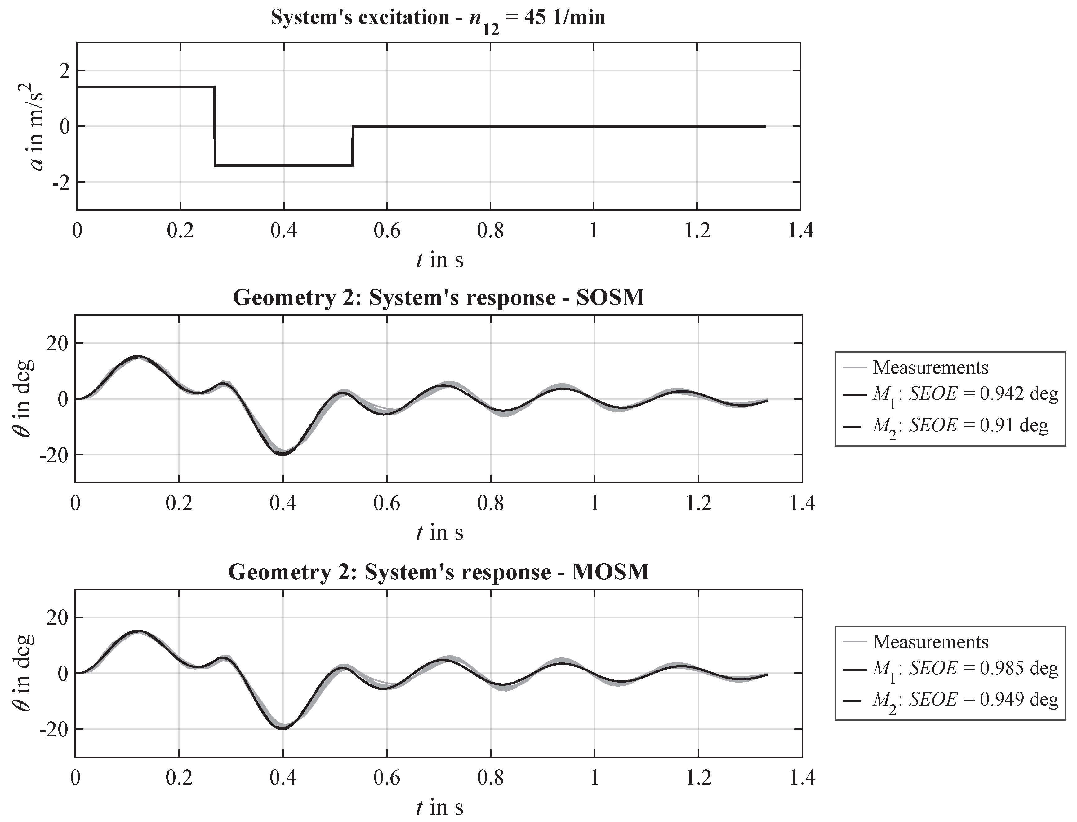
Figure 8 shows exemplarily the measured and simulated results for an operating speed of 45 1/min and the second geometry, as well as the related values for the SOSM and MOSM approaches. The simulated courses appear to fit very well to the measured courses, and the differences between the different model approaches are very small.
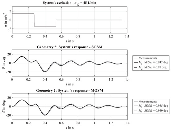
Figure 8.
Exemplarily results of measured and simulated courses for all different model approaches of Geometry 2 and 1/min.
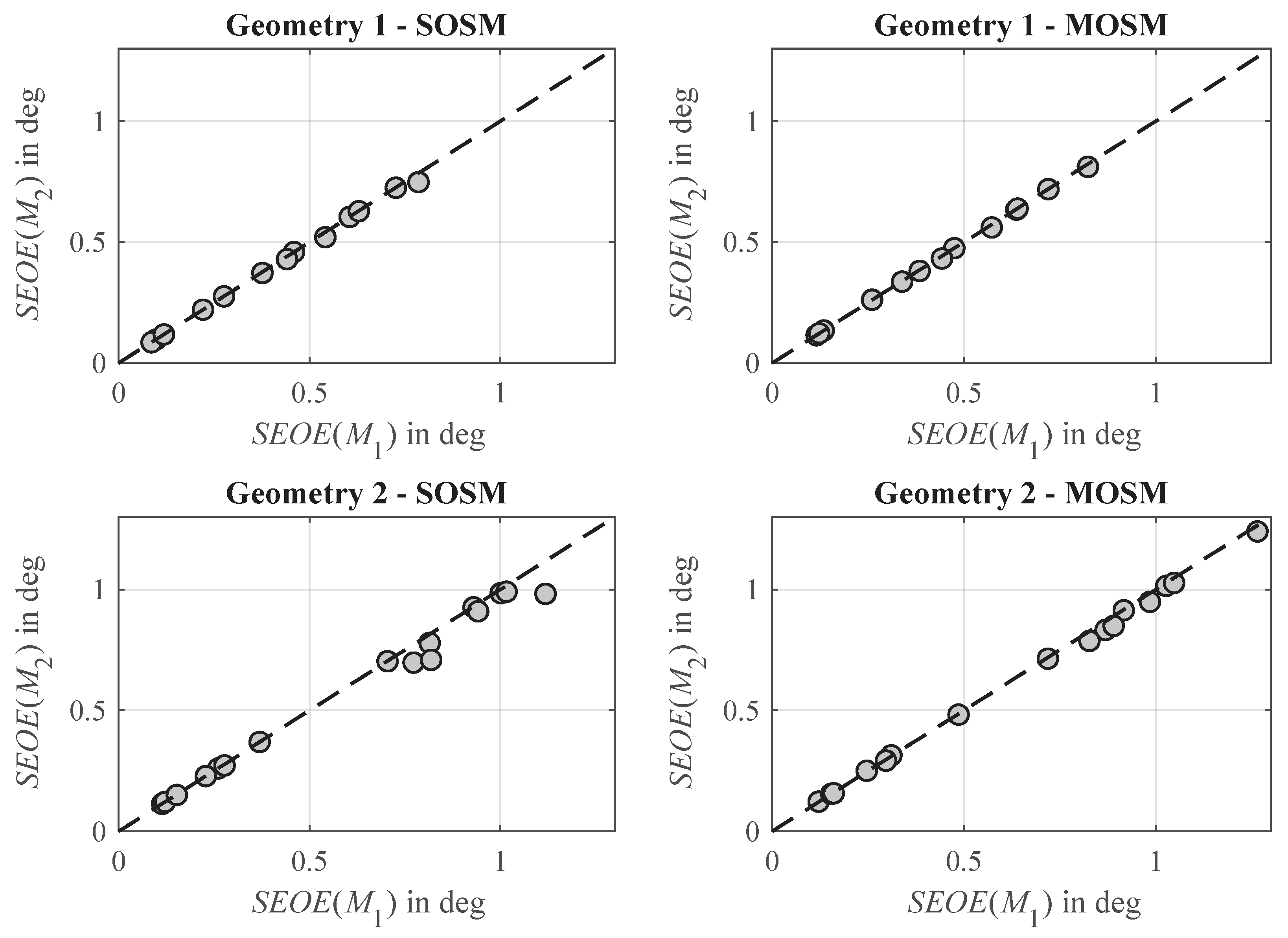
In order to get a better impression of the values determined for the different approaches and strategies for different operating speeds and geometries, Figure 9 shows the results for two exemplarily geometries. The results of the other geometries behave analogously and are therefore not shown.

Figure 9.
Determined standard error of estimate () values for the two different model approaches and strategies for all considered operating speeds and the two exemplarily geometries 1 and 2.
It can be seen that the values for model approaches 1 and 2 are essentially identical, since the data points lie approximately on the line . Furthermore, it can be noted that the MOSM strategy provides slightly higher values than the SOSM strategy. For a comparison of all results, Table 3 summarizes the maximum values for all approaches and geometries. In addition to that, the amount of necessary model parameters is stated. These quantities are identical for all geometries applying the MOSM strategy. Applying the SOSM strategy, the amount of necessary parameters depends on the maximum valid operating speed, which in turn depends on the considered geometry.

Table 3.
The results of model evaluations for different model approaches, strategies, and considered geometries as well as the amount of necessary parameters.
Hence, it can be summarized that, expectably, due to a higher amount of parameters, the SOSM strategy leads to better results than the MOSM strategy, and model approach leads to better results than . Thereby, better results are understood as smaller values. However, it has to be stated that the differences are nevertheless very small. Due to the very good ratio of minor model errors and a small number of model parameters, model approach in combination with the MOSM strategy will be treated in the following as the preferred solution and investigated during a model validation more closely.
4. Discussion
The question posed at the beginning of the present paper concerning the maximum possible operating speed up to which the assumption of a straight line for describing the fluid surface is valid can be answered with the help of the presented evaluation method. The determined deviations increase with increasing operating speed, since the waveform of the fluid surface assumes an increasing characteristic shape and thus deviates significantly from a straight line. The fact that the standard deviations of increase with the operating speed may indicate a higher sensitivity of the system to the initial state at higher operating speeds.
Another conclusion that can be derived from the results concerns the relationship between container width and maximum operating speed. With increasing container width, the maximum possible operating speed decreases. This is due to the fact that as the container width increases, the fluid volume to be conveyed increases as well. Due to the associated greater inertia, the characteristic surface waveform is formed at a lower motion’s profile velocity.
It has been shown that model approaches and both achieve good results, with the second approach having a free parameter in the form of a proportionality factor to reinforce the motion’s acceleration profile. Apparently, the factor given by the linearized pendulum equation is already a very good specification, which is represented almost identically by the free proportionality factor p. Therefore, no additional value is achieved in the model quality, as proposed in [23,24].
The second question formulated in the beginning concerns the applicability of the different model approaches for the whole range of valid operating speeds. Therefore, the two different strategies SOSM and MOSM were investigated. The SOSM strategy provides slightly better results, but those are hardly significant. From this it can be concluded that the model parameters can be regarded as constant within the valid operating speed range and that a model for the respective range is therefore sufficient for the considered application.
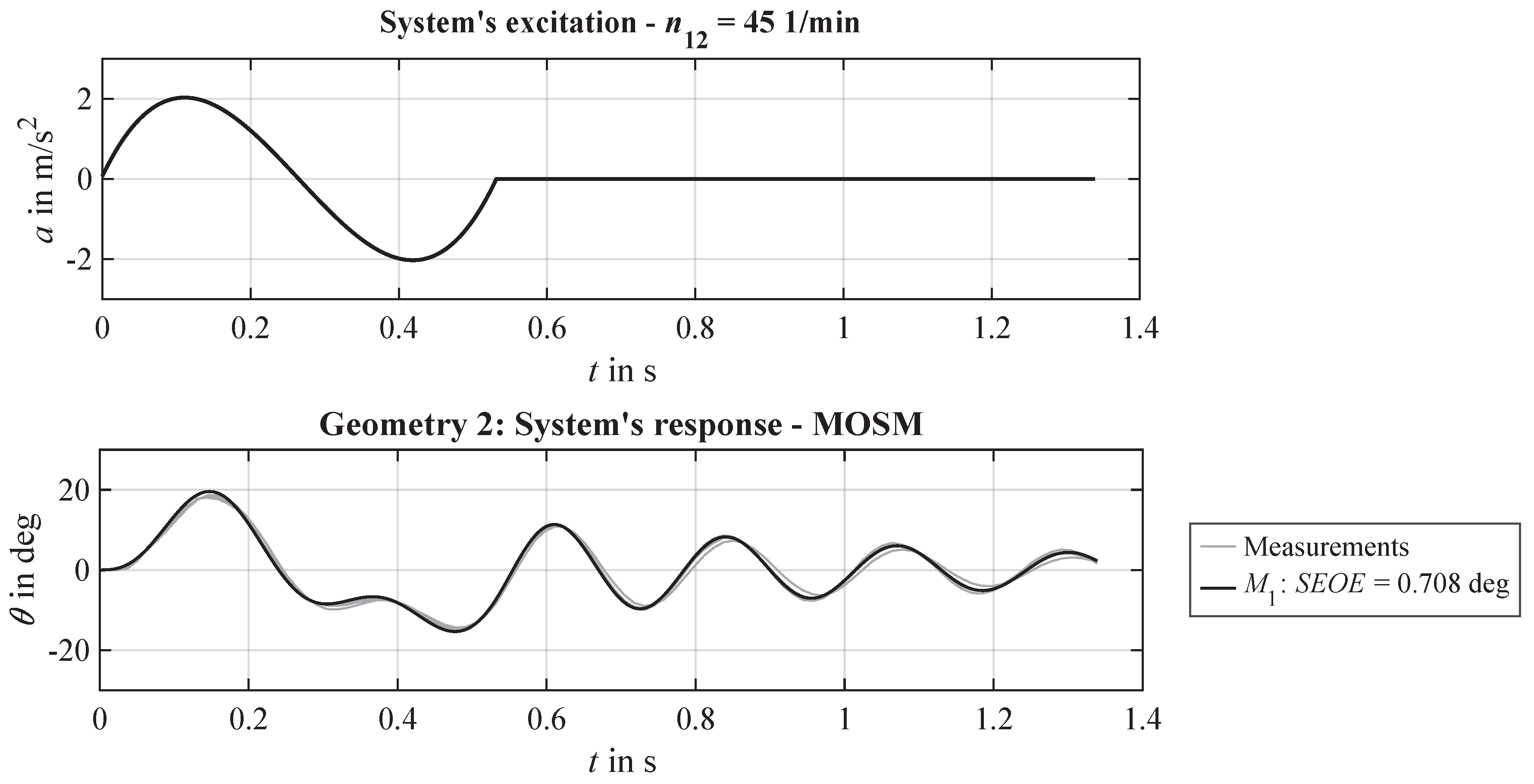
Finally, in the sense of a model validation, it should be discussed whether the models of approach in combination with the MOSM strategy of the different geometries derived from the acceleration pulse motion profile also provide similar simulation results for the validation quintic polynomial motion profile. To examine this, repeat tests are performed with , and the measurements are compared with the corresponding simulation results. The value is used again for quantification. In Figure 10, exemplarily simulation results and a comparison to measurements are shown for geometry 2 and operating speed 1/min. In principle, it can be stated that the dynamic behavior of the system is also well reproduced for this modified input. Furthermore, the value is similar to the derived from the parameter identification measurements (see Figure 8).
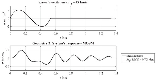
Figure 10.
Exemplarily validation results and value displayed for geometry 2 and an operating speed of n = 45 1/min, applying the Multiple-Operating-Speed Model (MOSM) strategy and model approach .
For a better comparison of all considered geometries and a corresponding assessment regarding the model’s applicability, Table 4 shows the results of the maximum values recorded for the parameter identification motion profile and the validation measurements. The respective values are proportional to each other, whereby the results for the validation evaluation are higher. This is understandable for two reasons. First, these system inputs have not been used for parameter identification. Second, the quintic polynomial motion has higher acceleration values, which is why the system response also assumes higher values and therefore model inaccuracies are of greater importance.

Table 4.
Results of investigations: for each geometry, the derived model parameters as well as the maximum operating speed are stated. Furthermore, the maximum values are given for both the derived model applied to the identification motion profile and that applied to the validation motion profile.
Nevertheless, this investigation shows that the derived models are well suited to simulate realistic system responses for arbitrary motion specifications that have not been used for parameter identification. Eventually, this means that the models can also be used for automated trajectory optimization in an expedient way, as initially required.
In order to get a better impression of the derived results and model parameters, they are shown in Figure 11 as a function of the varied fluid width w. In addition, an approximation equation is given in the literature [7] for the resulting first undamped natural frequency, which is supplementary illustrated in Figure 11:
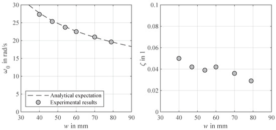
Figure 11.
Depiction of derived model parameters and dependent on the container’s width w. Furthermore, the analytical expectation of the angular natural frequency is displayed.
For describing the damping ratio , no approximation formula is known to the author’s knowledge.
The undamped natural frequency decreases by increasing the fluid’s width. It can be seen that there is very good agreement between the derived model parameter from the experiments and the predicted parameters from Equation (20). This observation fits the vibration theory, since it is well known that, with increasing mass, which results from a larger volume, natural frequency decreases. Therefore, the results are plausible. With one exception, the damping ratio also decreases with the fluid’s width. This coherence is evident by the decreasing influence of the dissipative frictional energy between the fluid and the container walls in relation to the total kinetic and potential energy, simultaneously with the fluid width.
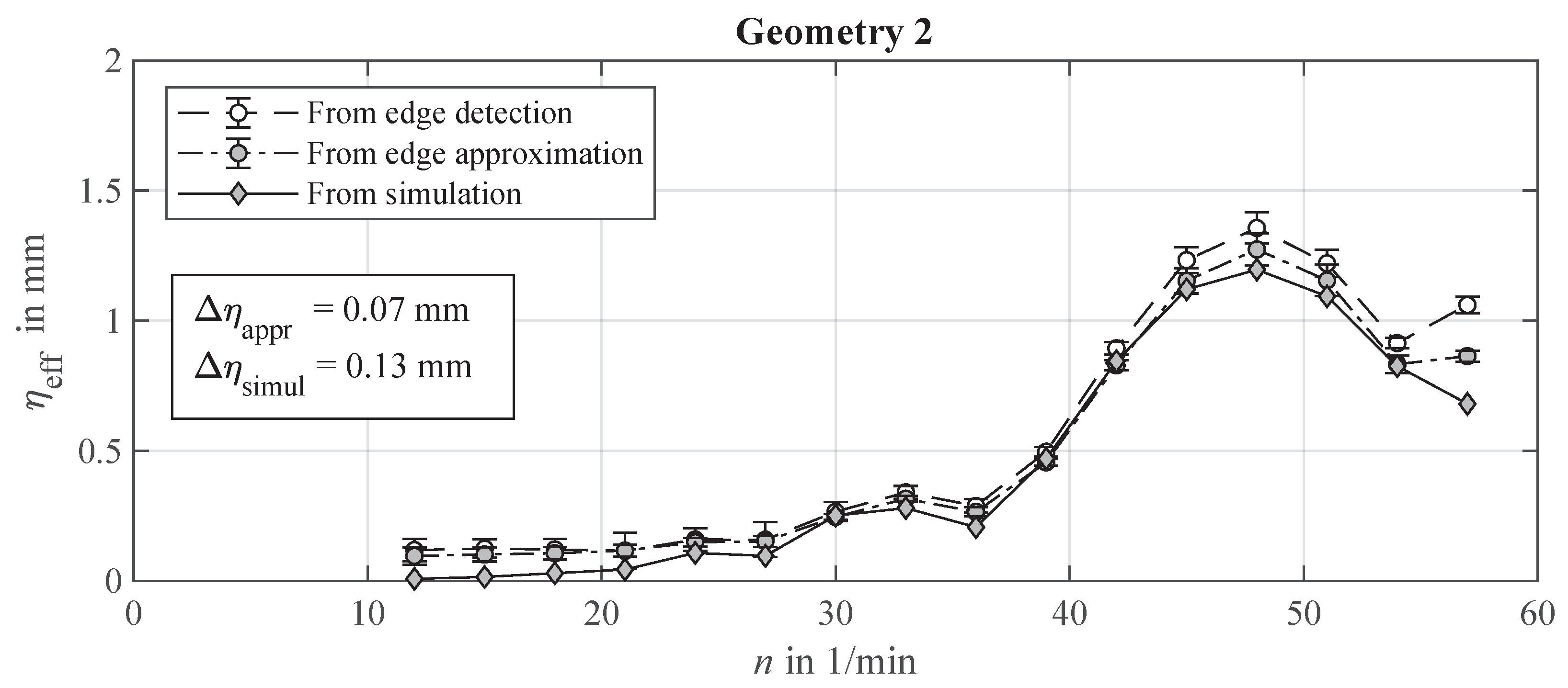
Whether the derived models are applicable for predicting the residual vibration had to be investigated. Therefore, the measure of introduced in Equation (17) was evaluated for the measured fluid edge, the line approximation, and the model response. An exemplarily result is displayed in Figure 12. Furthermore, the difference measures introduced in Equations (18) and (19) were calculated and are additionally shown. Overall a good accordance of the different measures can be seen, whereby expectably the difference measure is a bit greater than . In Table 5, these measures are shown for all investigated geometries. The evaluated differences are very small and hardly vary among the different geometries. Hence, in summary, the derived models are capable of predicting residual vibrations for motion profiles other than those used for parameter identification.

Figure 12.
Exemplarily evaluated mean differences between line approximation and simulation in comparison to the measured edge for applying the quintic polynomial motion profile that was not used for model parameter identification.

Table 5.
Summary of the evaluated effective fluid edge measures for all investigated geometries and their corresponding differences from approximation and model application.
5. Conclusions
The investigation of the deviations between the measured fluid surface and the approximated line allows for the determination of the model assumption previously assumed in the literature. Thus, a method has been presented, and it can be applied generically to determine model limits in terms of the applicable operating speed range. In addition, which previous model approaches in the form of ordinary differential equations are suitable for determining sloshing behavior over a determined operating speed range was investigated. It is shown that the simplest possible approach of the linearized pendulum equation is sufficient to describe the measured data. Finally, whether the derived models are also suitable for predicting the residual vibration for other motion profiles was confirmed. The presented methodical approach thus allows for the provision of models for automated motion optimization in packaging machines. This will be treated in future works as well as increasing the trajectory’s robustness by the consideration of parameter uncertainties.
Author Contributions
C.T. was responsible for writing the original draft of the present paper, the methodology, investigation, and visualizations. The funding acquisition, review, and editing of the manuscript as well as conceptualization were performed by J.-P.M. All authors have read and agreed to the published version of the manuscript.
Funding
This research was funded by the German Research Foundation under project number 182157057.
Acknowledgments
Special thanks are dedicated to the Chair of Machine Tools Development and Adaptive Controls, TU Dresden for lending the measurement equipment.
Conflicts of Interest
The authors declare that there is no conflict of interest. The funders had no role in the design of the study; in the collection, analyses, or interpretation of data; in the writing of the manuscript; or in the decision to publish the results.
Nomenclature
| Damping ratio | |
| Undamped natural angular frequency | |
| Deflection of fluid surface | |
| s | Horizontal path of transport motion |
| t | Time |
| x | Horizontal coordinate |
| Time derivative of horizontal coordinate | |
| Second time derivative of horizontal coordinate | |
| y | Vertical coordinate |
| Container’s conveyed stroke in one cycle | |
| b | Ratio of motion time to cycle time |
| Cycle time | |
| T | Kinetic energy |
| n | Operating speed |
| Container’s geometry | |
| U | Potential energy |
| Vector of generalized coordinates | |
| Vector of forces acting on the generalized coordinates | |
| Measured fluid surface’s vertical displacement | |
| Approximated fluid surface’s vertical displacement | |
| Effective value of | |
| Difference of effective value | |
| w | Fluid volume’s width |
| d | Damping constant |
| F | Actuating force |
| g | Gravitational acceleration |
| Pendulum’s length | |
| Pendulum’s mass | |
| Linear drive’s mass | |
| L | Lagrangian |
| D | Dissipative Energy |
| a | Motion’s profile acceleration |
| p | Model parameter describing the acceleration’s magnification |
| i | Index for stating the discrete horizontal coordinates |
| j | Index for stating the discrete time |
| k | Index for stating the experiment’s repetition |
| u | Index for stating the operating speed |
| v | Index for stating the container’s geometry |
| o | Index for stating an item of the generalized vector |
| I | Number of discretization points for horizontal coordinate |
| J | Number of captured frames per measurement |
| Number of captured frames per measurement during motion phase | |
| K | Number of repetitions |
| FR | Frame rate |
| Standard error of estimate | |
| SOSM | Single-operating-speed model |
| MOSM | Multiple-operating-speed model |
References
- Abramson, H.N.E. Dynamic Behavior of Liquids in Moving Containers with Applications to Propellants in Space Vehicle Fuel Tanks; Technical Report; NASA: Washington, DC, USA, 1966.
- Abramson, H.N.; Chu, W.H.; Kana, D.D. Some Studies of Nonlinear Lateral Sloshing in Rigid Containers. J. Appl. Mech. 1966, 33, 777–784. [Google Scholar] [CrossRef]
- Eswaran, M.; Saha, U.K. Sloshing of liquids in partially filled tanks—A review of experimental investigations. Ocean Eng. 2011, 1, 131–155. [Google Scholar] [CrossRef]
- DIN. DIN 8743: Packaging Machines and Packaging Installations, Time Related Definitions, Reference Factors and Calculation Fundamentals; DIN: Berlin, Germany, 2007. [Google Scholar]
- Rexroth, B. How Adaptive Systems Unlock Big Producitivity Gains; Technical Report; Bosch Rexroth Group: Lohr am Main, Germany, 2014. [Google Scholar]
- Bossel, H. Systems and Models: Complexity, Dynamics, Evolution, Sustainability; Books on Demand GmbH: Norderstedt, Germany, 2007. [Google Scholar]
- Ibrahim, R.A. Liquid Sloshing Dynamics: Theory and Applications; Cambridge University Press: Cambridge, UK, 2005. [Google Scholar] [CrossRef]
- Kolaei, A. Dynamic Liquid Slosh in Moving Containers. Ph.D. Thesis, Concordia University, Montreal, QC, Canada, 2014. [Google Scholar]
- Ibrahim, R.A. Recent Advances in Physics of Fluid Parametric Sloshing and Related Problems. J. Fluids Eng. 2015, 137, 090801. [Google Scholar] [CrossRef]
- Green, S.T. A Comparison of Methods for Estimating Slosh Model Parameters from CFD Simulations. In Proceedings of the 2018 Joint Propulsion Conference, Cincinnati, OH, USA, 9–11 July 2018. [Google Scholar] [CrossRef]
- Sanapala, V.; Mohanraj, R.; Velusamy, K.; Patnaik, B. Numerical simulation of parametric liquid sloshing in a horizontally baffled rectangular container. J. Fluids Struct. 2018, 76, 229–250. [Google Scholar] [CrossRef]
- Stephen, J.J.; Sannasiraj, S.A.; Sundar, V. Numerical modeling of nonlinear sloshing of liquid in a container coupled with barge subjected to regular excitation. J. Hydrodyn. 2019, 31, 999–1010. [Google Scholar] [CrossRef]
- He, R.; Zhang, E.; Fan, B. Numerical analysis on the sloshing of free oil liquid surface under the variable conditions of vehicle. Adv. Mech. Eng. 2019, 11, 1687814019829967. [Google Scholar] [CrossRef]
- Terashima, K.; Schmidt, G. Motion control of a cart-based container considering suppression of liquid oscillations. In Proceedings of the 1994 IEEE International Symposium on Industrial Electronics (ISIE’94), Santiago, Chile, 25–27 May 1994; pp. 275–280. [Google Scholar] [CrossRef]
- Feddema, J.T.; Dohrmann, C.R.; Parker, G.G.; Robinett, R.; Romero, V.J.; Schmitt, D.J. Control for slosh-free motion of an open container. Control Syst. IEEE 1997, 17, 29–36. [Google Scholar] [CrossRef]
- Hamaguchi, M.; Terashima, K.; Nomura, H. Optimal Control of Transferring a Liquid Container for Several Performance Specifications. Trans. Jpn. Soc. Mech. Eng. Ser. C 1994, 60, 1668–1675. [Google Scholar] [CrossRef]
- Yano, K.; Yoshida, T.; Hamaguchi, M.; Terashima, K. Liquid Container Transfer Considering the Suppression of Sloshing for the Change of Liquid Level. IFAC Proc. Vol. 1996, 29, 701–706. [Google Scholar] [CrossRef]
- Troll, C.; Schebitz, B.; Majschak, J.P.; Döring, M.; Holowenko, O.; Ihlenfeldt, S. Commissioning new applications on processing machines: Part II – implementation. Adv. Mech. Eng. 2018, 10, 1687814018754955. [Google Scholar] [CrossRef]
- Troll, C.; Tietze, S.; Majschak, J.P. Investigation on the Application of Operating Speed Dependent Motion Profiles in Processing Machines at the Example of Controlling Liquid Slosh. In Advances in Mechanism and Machine Science; Uhl, T., Ed.; Springer International Publishing: Cham, Switzerland, 2019; pp. 1909–1918. [Google Scholar]
- Barron, R.; Chng, S.W.R. Dynamic Analysis and Measurement of Sloshing of Fluid in Containers. J. Dyn. Syst. Meas. Control 1989, 111, 83–90. [Google Scholar] [CrossRef]
- Canny, J. A Computational Approach To Edge Detection. IEEE Trans. Pattern Anal. Mach. Intell. 1986, 6, 679–698. [Google Scholar] [CrossRef]
- Florian, R.V. Correct Equations for the Dynamics of the Cart-Pole System; Center for Cognitive and Neural Studies (Coneural): Cluj-Napoca, Romania, 2005. [Google Scholar]
- Dietze, S.; Schmidt, F.J. Entwurf zur Optimalsteuerung offener Behälter zum Fördern von Fluiden in Verarbeitungsmaschinen. In Technical Report MATH-NM-13-1997; Technische Universität Dresden: Dresden, Germany, 1997. [Google Scholar]
- Grundelius, M. Methods for Control of Liquid Slosh. Ph.D. Thesis, Department of Automatic Control, Lund Institute of Technology, Lund, Sweden, 2001. [Google Scholar]
- Nocedal, J.; Wright, S.J. Numerical Optimization, 2nd ed.; Springer: New York, NY, USA, 2006. [Google Scholar]
- Sewell, G. The Numerical Solution of Ordinary and Partial Differential Equations, 2nd ed.; John Wiley & Sons: Hoboken, NJ, USA, 2005. [Google Scholar]
- Bronstein, I.N.; Semendyayev, K.A.; Musiol, G.; Mühlig, H. Handbook of Mathematics; Springer: Berlin/Heidelberg, Germany, 2007; Volume 5. [Google Scholar]
© 2020 by the authors. Licensee MDPI, Basel, Switzerland. This article is an open access article distributed under the terms and conditions of the Creative Commons Attribution (CC BY) license (http://creativecommons.org/licenses/by/4.0/).

