Air Quality Prediction in Smart Cities Using Machine Learning Technologies Based on Sensor Data: A Review

Abstract

The influence of machine learning technologies is rapidly increasing and penetrating almost in every field, and air pollution prediction is not being excluded from those fields. This paper covers the revision of the studies related to air pollution prediction using machine learning algorithms based on sensor data in the context of smart cities. Using the most popular databases and executing the corresponding filtration, the most relevant papers were selected. After thorough reviewing those papers, the main features were extracted, which served as a base to link and compare them to each other. As a result, we can conclude that: (1) instead of using simple machine learning techniques, currently, the authors apply advanced and sophisticated techniques, (2) China was the leading country in terms of a case study, (3) Particulate matter with diameter equal to 2.5 micrometers was the main prediction target, (4) in 41% of the publications the authors carried out the prediction for the next day, (5) 66% of the studies used data had an hourly rate, (6) 49% of the papers used open data and since 2016 it had a tendency to increase, and (7) for efficient air quality prediction it is important to consider the external factors such as weather conditions, spatial characteristics, and temporal features.

1. Introduction

The numbers show that more and more people are moving to cities. According to United Nations (UN) urban population as of 2018 is about 55.3% [1] and by 2050 it will become 68% [2]. Growth of urbanization causes some problems related to different aspects of life, such as transportation, health care, air quality, etc. The smart city concept was created to solve these problems, which by integrating Information and Communication Technology (ICT) with citizens and existing resources can support sustainable development and life quality improvement. There are different definitions describing smart cities, such as ‘A smart city is a city in which there are six main components including smart economy, smart transportation, smart environment, smart citizens, smart life, and smart management’ [3] or ‘The use of smart computing technologies to make the critical infrastructure components and services of a city-which include city administration, education, healthcare, public safety, real estate, transportation, and utilities—more intelligent, interconnected, and efficient’ [4]. Using the services built around the smart city notion allows us to capture a huge amount of data about the current situation and to see the real picture all over the city. The availability of data provided by sensors is a significant feature of smart cities [5,6].

From the above-mentioned issues and definitions, we can notice that air quality is considered to be an essential component in the smart city concept. Air quality has become a massive problem in many areas. According to World Health Organisation (WHO), every year more than seven million persons are dying because of this problem and more than 80% of urban areas population lives in places where air quality rises over WHO guideline limits [7]. As reported by Apte et al. [8], the global and national life expectancy has been reduced because of air pollution. The study shows that in 2016 particulate matter with a diameter equal to 2.5 micrometres (PM_2.5) reduced global life expectancy about 1.2–1.9 years in some polluted countries of Asia and Africa. According to the following research [9] PM_2.5 has severe effects for human life, becoming the reason of about 3% of mortality from cardiopulmonary disease, 5% of mortality from cancer of the trachea, bronchus, and lung, and about 1% of mortality from acute respiratory infections in children under five year. This study [10] presents that PM_2.5 in 2015 was the fifth-ranking mortality risk factor. Therefore, it is a crucial problem to prevent or reduce consequences caused by air pollution. Having information about air quality will induce us to make protective measures; it can lead the population to apply their daily activities in the places which are less polluted (by escaping high polluted areas). However, analysing the data, giving smart solutions remains as a challenging task. Thus, it is essential to apply productive methods and techniques for more effectively and more efficiently analysing big data, converting the invisible to visible, and extracting information hidden behind data.

This paper aims to review the articles related to air pollution prediction in smart cities using machine learning techniques, to make a comparison of methodologies that different authors have been used and to get an overall idea about applied approaches. The usage of machine learning techniques in this area has begun to be actively developed, and many studies and observations have been done, which is conditioned by the importance of the field. The combination of all the information will help us to detect the tendency, to find out the innovations applied in the research area, which, in turn, will direct and guide us for future exploration. We selected the most relevant papers from the most popular databases by applying different filters based on several criteria, which are represented in detail in the next section. The comprehensive study of those papers prompts us to highlight the following outcomes: (1) the usage of the advanced and sophisticated machine learning techniques is increasing, contrary to simple models; (2) as a case study compared to other countries, China was the primary country; (3) among the other prediction elements, PM_2.5 was the principal target element; (4) the most predicted time resolution is 24 h; (5) in the most cases data provided by sensors have an hourly rate; (6) for effective prediction it would be better to combine air quality data with other types of data; and (7) considering the emergence of open data portals, more works have recently appeared using open data.

The rest of the paper is organised as follows. Section 2 explains methodology. Section 3 describes each revised paper, including the main goal, applied methodology and obtained results. Section 4 includes a discussion based on the result of reviewing the selected papers. Finally, in Section 5 we included the conclusion.

2. Methods

This section describes the methodology applied during the review. First of all, research questions are defined, which as a guiding tool navigated us through all time. Afterwards, the search strategy is presented.

2.1. Research Questions

The research questions, which are considered to be the fundamental basis of the research for defining research strategies and for directing the research process, are presented below:

• Which machine learning techniques are used to predict air quality in the smart city domain?
• How do the proposed methods handle different types of data in terms of air pollution?
• What temporal resolutions were analysed with the proposed techniques?

2.2. Search Strategy and Inclusion/Exclusion Criteria

To select and research relevant papers, first of all, we selected databases, including Scopus and IEEE Xplore repositories. Then, we defined the searching terms, and the entry query was as follows: ‘Machine Learning’ AND ‘Air Quality Predict*’ OR ‘Air Pollut*’. The next step was year and source type restrictions by selecting journal papers and conference proceedings published since 2002. The output of this step provided 316 papers.

It should be noted that recently Rybarczyk and Zalakeviciute published a paper about ’Machine learning approaches for outdoor air quality modelling: A systematic review’ [11]. By reviewing this paper, we have defined key features which were taken into consideration during our study. In the first place, we have narrowed the scope of the models by choosing only forecasting models, while the authors mentioned above also included papers concentrated on the estimation models. Another reduction is that we selected papers in which only sensor data in the smart cities context are being used. After these steps and after excluding duplicated manuscripts and reviewing titles and abstracts, the filtration output reached 131. Finally, applying quality assessment, irrelevant papers were excluded, and as a result, we had 41 selected papers. The key questions, on which we focused during the quality assessment, are listed below:

• Are the research aims clearly specified?
• Was the study designed to achieve these aims?
• Are the used techniques clearly described and their selection justified?
• Are the data collection methods adequately described?
• Is the purpose of the data analysis clear?
• Are the findings convincing?
• How clear are the links between data, interpretation and conclusions?

The inclusion and exclusion criteria used during the review are listed in

Table 1. Inclusion and Exclusion Criteria.

Inclusion Criteria	Exclusion Criteria
Papers written in English	Non-English written papers
Publications in scientific conferences or scientific journals	Non-reviewed papers, editorials, presentations
Publications since 2002	Publications before 2002
Works focused on smart city services enabled by Internet of Things (IoT)	Papers not related to smart city services enabled by IoT
Papers that propose IoT-based solution(s) for smart city services	Papers with no concrete solution/s
	Duplicated studies

and the overall workflow of the review is represented in Figure 1.

3. Results

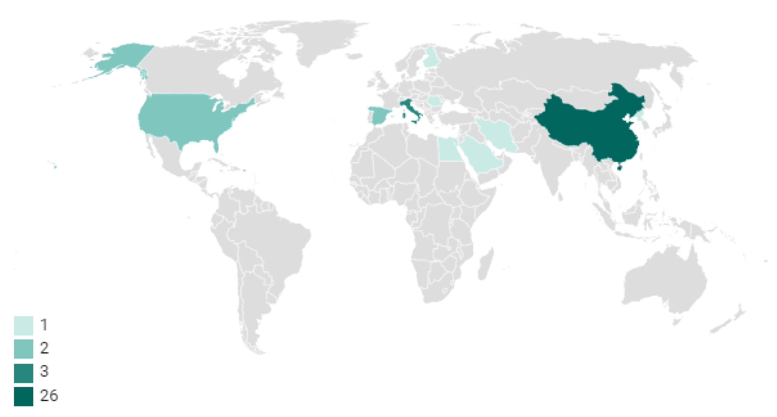
3.1. Overview of the Included Studies

After examining the works, the following aspects were extracted: publication years, countries which were served as a case study and machine learning algorithms applied in the papers, which will enable us to obtain a general picture of the present scene.

Regarding publication years, Figure 2 shows the progress of the publications related to air quality prediction in smart cities using machine learning techniques based on sensor data.

About countries, Figure 3 on the world map demonstrates the countries where are located the cities which were served as a case study in the publications. It can be noted that China is leading this kind of research works with 26 papers, followed by Italy (3 papers), Spain (2 papers), USA (2 papers), South Korea (1 paper), Iran (1 paper), Egypt (1 paper), Romania (1 paper), Qatar (1 paper), Finland (1 paper) and Saudi Arabia (1 paper).

Related to the algorithms, we categorised the applied methods based on machine learning algorithms. Figure 4 shows the output of categorization (Neural Network (NN), Regression, Ensemble, Hybrid Model, Others). It can be seen that the neural network is leading other algorithms by use in 17 papers. The next most used algorithm is regression, applied in 11 manuscripts, then ensemble in 10 papers, hybrid models in five papers, and Others are two papers, one of which is focused on the regularization and optimization, and the other study applied multinomial naïve bayes and multinomial logistic regression methods.

3.2. Exhaustive Descriptions of Included Studies

This section includes a brief description of each selected paper, involving applied methods and obtained results. We grouped the papers based on machine learning algorithms represented in Figure 4 (NN, Regression, Ensemble, Hybrid Model, Others).

3.2.1. Group 1: Neural Network (NN)

Prediction of Air Pollution Concentration Based on mRMR and Echo State Network [12]: to predict PM_2.5, Xu and Ren employed a Supplementary Leaky Integrator Echo State Network (SLI-ESN) which can memorise historical information. First of all, they used minimum Redundancy Maximum Relevance (mRMR) feature selection method to solve a problem related to data redundancy, which increased computational speed. Then they applied phase space reconstruction to extract evolutionary information of relevant variables, and finally, to perform prediction, SLI-ESN was applied. The following methods were used for comparison purposes: Echo State Network (ESN), Leaky Integrator Echo State Network (LI-ESN), Extreme Learning Machine (ELM), Hierarchical ELM and Stacked Auto-Encoder. The dataset consisted of air pollution (PM_2.5, particulate matter with diameter equal to 10 micrometers (PM₁₀), nitrogen dioxide (NO₂), carbon monoxide (CO), ground-level ozone (O₃), sulfur dioxide (SO₂)) and meteorological (temperature, pressure, humidity, wind speed, wind direction) data. The predictive indicators used for evaluating the model were Root Mean Square Error (RMSE), Normalised Root Mean Square Error (NRMSE), Mean Absolute Error (MAE), Symmetric Mean Absolute Percentage Error (SMAPE) and Pearson correlation coefficient (R). The results showed that compared to other methods, SLI-ESN performed better results. In addition, the authors compared methods, in terms of the time factor, and the results showed that ESN and ELM based methods were faster than deep learning model, because the latter one consumes much time in training step for optimal subset selection and model optimization. The proposed method was not the fastest one, but it was in an acceptable time frame. About the limitations, the main problem was that for the longer term, the result was not satisfactory.

Spatiotemporal Prediction of PM2. Five Concentrations at Different Time Granularities Using IDW-BLSTM [13]: Ma et al. applied the combination of Bi-directional Long Short-Term Memory (BLSTM) network and the Inverse Distance Weighting (IDW) technique for the spatiotemporal prediction of PM_2.5 concentration at different time granularities (hourly, daily, and weekly granularities). The proposed method was compared to AutoRegressive Integrated Moving Average (ARIMA), ElasticNet, Support Vector Regression (SVR), Gradient Boosting Decision Tree (GBDT), Artificial Neural Network (ANN), Recurrent Neural Network (RNN), Long Short-Term Memory (LSTM), BLSTM, Convolutional Neural Network-LSTM (CNN-LSTM). The authors used different indicators, including RMSE, MAE and Mean Absolute Percentage Error (MAPE) to evaluate the methods. The results showed that IDW-BLSTM, CNN-LSTM, BLSTM, LSTM, and RNN had better performances compared to other methods. Overall, the IDW helped BLSTM to improve accuracy by 5.6%, and the final results of the proposed methods were RMSE-8.24, MAE-4.80, MAPE(%)-9.01. This study included analysis related to finding optimal window size for different temporal granularities. The result showed that when the window size was five, it was the optimal size for the hourly as well as for daily and weekly granularities. The limitation was that only the historic air pollution data were used and other relevant data (the meteorological and urban information) were not included.

Air Pollution Forecasting Using a Deep Learning Model Based on 1D Convnets and Bidirectional GRU [14]: Tao et al. introduced short-term forecasting method for PM_2.5 which included the Convolutional-based Bidirectional Gated Recurrent Unit (CBGRU) combined with 1D convnets and Bidirectional Gated Recurrent Unit (BGRU) neural networks. The former one was responsible for feature extraction, and the latter one was for time series forecasting. For checking the effectiveness of the method, the authors compared it to SVR, Gradient Boosting Regression (GBR), Decision Tree Regression (DTR), simple RNN, LSTM, Gated Recurrent Unit (GRU) and BGRU. The data used in this study were from the machine learning repository at the University of California, Irvine (UCI) [15] and meteorological data from Beijing Capital International Airport. RMSE, MAE and SMAPE were used for evaluation purposes. Comparing to the traditional ones, the prediction results demonstrated that the error of the CBGRU model was lower, including RMSE-14.5319, MAE-10.4789 and SMAPE-0.2055.

A Deep CNN-LSTM Model for Particulate Matter (PM_2.5) Forecasting in Smart Cities [16]: to forecast PM_2.5, the combination of Convolutional Neural Network (CNN) and LSTM was applied. CNN was responsible for features extraction, LSTM was for analysing the extracted features and for estimating the PM_2.5 concentration of the next point in time. The method proposed here (APNet) used PM_2.5 concentration, cumulated wind speeds, and cumulated hours of rain over the last 24 h in order to predict PM_2.5 for the next hour. Support Vector Machine (SVM), Random Forest (RF), Decision Tree (DT), Multilayer Perceptron (MLP), CNN, and LSTM were used for comparison purposes. As an evaluation metrics, the authors selected MAE, RMSE, R and Index of Agreement (IA). The results showed that, although CNN and LSTM separately achieved good results, the combination of them, the proposed CNN-LSTM model (APNet) was better having the following results: MAE-14.63446, RMSE-24.22874, R-0.959986, IA-0.97831.

A Sequence-to-Sequence Air Quality Predictor Based on the n-Step Recurrent Prediction [17]: taking into account that sequence-to-sequence (seq2seq) had some problems (slow training speed, error accumulation), Liu et al. proposed to use an Attention-based Air Quality Predictor (AAQP) with n-step recurrent prediction. To accelerate the training process, RNN in encoder was replaced with a Fully Connected (FC) layer and also considering that FC layer was not as powerful as RNN during the process of sequential data, position embedding was applied. To improve the accuracy, n-step recurrent prediction was applied. MAE and determination coefficient (R²) were used as performance metrics. The following methods were used to compare and measure the proposed method: ANN, SVM, GRU, LSTM, seq2seq, seq2seq-mean, seq2seq-attention and n-step AAQP. The Olympic Center station (smaller fluctuations of PM_2.5) and Dongsi station (big fluctuations of PM_2.5) were selected as the target stations. The results showed that attention-based models demonstrated better results and also recurrent prediction induced better results compared to direct prediction. The proposed AAQP (GRU) method in the Olympic Center station had similar performances to the original seq2seq model with attention. According to the MAE score, the best performance was seq2seq-attention (GRU)-33.109, and for R² was seq2seq-attention(GRU)-0.253. In the Dongsi station according to MAE score and R², the best performance was 1-step AAQP (GRU)-41.468 and 0.228 respectively, which confirmed that proposed AAQP (GRU) method was better compared to other methods. Related to the steps analysis, the results showed that 12-step AAQP was the best. The authors also compared training and prediction time for each model. The results showed that training time (s) of 12-step AAQP (GRU) and the prediction time of 12-step AAQP (LSTM) had better performances. Concerning future work, it was suggested to work on spatial attention and to collect more weather forecast data.

An End-to-End Adaptive Input Selection With Dynamic Weights for Forecasting Multivariate Time Series [18]: presents the Adaptive Input Selection with Recurrent Neural Network (AIS-RNN) for multivariate time series forecasting. The model consisted of two parts; the first model generated context-dependent importance weights for selecting proper inputs; afterwards, the second model based on the inputs predicted the target variable. For the latter part Elman networks (simple RNN), LSTM and GRU were applied. RMSE, MAE and MAPE were applied to estimate model performances. The dataset used in this research consisted of 3 different types: financial, energy use of appliances and air quality dataset. The latter one was taken from the machine learning repository at UCI [19]. For comparison purposes the following methods were taken: LSTM, GRU, RNN, SVM, RF, AdaBoost, DT based on Recursive Feature Elimination, VAR-based and without anything, and also LSTM, RNN, GRU based on AIS-RNN. The results showed that the proposed model outperformed other models. As future work, the authors proposed to extend AIS-RNN as an end-to-end ensemble model.

Prediction of Urban PM_2.5 Concentration Based on Wavelet Neural Network [20]: focuses on prediction of PM_2.5 using Wavelet Neural Network (WNN). Different techniques were chosen in order to evaluate the effectiveness of WNN, including ELM, Fuzzy Neural Network (FNN) and Least Squares Support Vector Machine (LSSVM). The dataset contained hour average concentration of temperature, relative humidity, O₃, CO, NO₂, SO₂, PM₁₀ and PM_2.5. Firstly, the Pearson correlation and the bilateral significance test were used to calculate the correlation between PM_2.5 and other pollutants. After inputting PM₁₀, CO, NO₂, SO₂ and O₃, temperature and relative humidity were considered for predicting the concentration of PM_2.5. For evaluating the prediction models, the statistical parameter of R², RMSE, and MAPE were chosen. Comparing to other methods, the results showed that detection results based on WNN were more accurate, only in terms of R² for 1 hour the FNN had comparatively better results (0.099). However, making WNN still is challenging because of the determination of proper wavelet basis function and hidden layer nodes.

A Deep Belief Network Based Model for Urban Haze Prediction [21]: Lu et al. proposed a Deep Belief Network (DBN) model to improve urban haze prediction (DBN-based urban haze prediction: DBN-H). Multilayer restricted Boltzmann machines and a single-layer back propagation network were applied. For meteorological data prediction, competitive adaptive-reweighed method was applied. For evaluation purposes were used R and MAE. In terms of haze content, PM_2.5 and PM₁₀ were taken, and in terms of meteorological content, wind speed, wind direction, temperature, humidity, light, and atmospheric pressure were obtained for the period of 2016-2017. Multiple regression, ARMA, Classification and Regression Tree, and NN were applied for comparison purposes. The results showed that DBN-H outperformed other methods, having R-0.767 and MAE-26.5 $mu$g/m${}^3$ results. Overall, DBN-H model provided a correlation result with 18% better than others, and MAE was decreased by 15.7 $\mu$g/m${}^3$. As a limitation, the lack of data was reported.

Deep Distributed Fusion Network for Air Quality Prediction [22]: Yi et al. offered the Deep Neural Network (DNN)-based approach consisted of a spatial transformation component and a deep distributed fusion network. The model was applied for 48 hour fine-grained air quality forecasts for more than 300 Chinese cities. Air quality data consisted of hourly collected elements, including PM_2.5, PM₁₀, NO₂, CO, O₃, and SO₂. A meteorological dataset consisted of weather (sunny, cloudy, overcast, foggy, snow, small rain, moderate rain, and heavy rain), humidity, temperature, pressure, wind speed, and wind direction was used. Weather forecast dataset consisted of weather, temperature, wind strength and wind direction. The proposed model was compared to the following methods: ARIMA, lasso, GBDT, FFA [23], LSTM, DeepST [24], DMVST-Net [25], DeepSD [26], DeepFM [27], WFM [28]. As an evaluation, metrics accuracy (ACC) and MAE were selected. The proposed approach outperformed other methods. The final results had 2.4%, 12.2%, and 63.2% relative accuracy improvements on short-term, long-term and sudden changes prediction, respectively compared to the previous system. Regarding future work, the long-term sudden changes prediction was considered.

Prediction of Air Pollutants Concentration Based on an Extreme Learning Machine: The Case of Hong Kong [29]: to increase air pollution prediction Zhang and Ding applied the extreme learning machine which performed good generalization with fast learning speed. The dataset used in this study included air quality (NO₂, nitrogen oxide (NO_x), O₃, PM_2.5, SO₂) and meteorological (temperature, wind speed, wind direction, relative humidity) data during the period of 2010–2015. The following parameters were applied in order to evaluate the proposed methods: MAE, RMSE, IA, and R². Compared to FeedForward Neural Network based on Back Propagation (FFANN-BP) and Multiple Linear Regression (MLR), the proposed method performed better.

Relevance analysis and short-term prediction of PM_2.5 concentrations in Beijing based on multi-source data [30]: focuses on the short-term prediction of PM_2.5 in Beijing. Multivariate statistical analysis method and Back Propagation Neural Network (BPNN) were applied in order to study correlation analysis. Afterwards, ARIMA was applied for predicting PM_2.5. The dataset consisted of air quality data (CO, NO₂, SO₂, PM₁₀), meteorological data (average rainfall, daily mean temperature, average relative humidity, average wind speed, maximum wind speed) and social media data (microblog data) collected during January and December in 2014. To analyse the correlation, the authors used R and the Spearman Correlation Coefficient and to evaluate the method RMSE was applied, which reached to 6.76 mg/m${}^3$.

Evolving Keras Architectures for Sensor Data Analysis [31]: presents the genetic algorithm for the architecture of deep neural networks using the KERAS library [32]. Applying air pollution data, the results showed that the proposed model could increase the accuracy of the air pollution prediction. The target pollutants were CO, NO₂, NO_x, benzene (C₆H₆), and non-methane hydrocarbons (NMHC). Compared to SVM and selected fixed architectures, the proposed method performed better.

Forecasting PM_2.5 Concentration using Spatio-Temporal Extreme Learning Machine [33]: by taking into account fast training, fewer configuration parameters, and ease of obtaining global optima, Spatio-Temporal Extreme Learning Machine (STELM) method was applied for enhancing forecasting of PM_2.5 for the next 72 hours. The dataset consisted of air quality data (NO₂, CO, SO₂, O₃, PM₁₀, and PM_2.5) and meteorological spatio-temporal sequences (temperature, humidity, wind direction, wind force, and precipitation) collected during April and May in 2014. Mean Relative Error (MRE) and MAE were used to evaluate the proposed method. Overall, the precision in the first 12, 24, 48, 72 hours were 82%, 78%, 71%, and 63%, respectively.

Urban Air Pollution Monitoring System With Forecasting Models [34]: aims to monitor urban air pollution and based on the results to make a prediction. Shaban et al. applied the following machine learning algorithm, including SVM, M5P, and ANN with univariate and multivariate models to forecast O₃, NO₂, and SO₂ for the next 1, 8, 12, and 24 h. The data were collected every 15 min. To compare the methods, the following metrics were used, including Prediction Trend Accuracy (PTA), RMSE and NRMSE. The results showed that M5P outperformed other methods. Additionally, the results confirmed that the multivariate approach had better performances compared to the univariate approach.

Air Quality Forecasting using Neural Networks [35]: Zhao et al. suggested to apply extreme learning machine-based approach to forecast air quality. The case study was Helsinki, and the data included hourly air quality data (nitric oxide (NO), O₃, PM₁₀, PM_2.5) and meteorological data (relative humidity, pressure, temperature, and wind). Taking into account the challenges related to big data analysis, the authors applied forward selection in order to select most correlated variables, later by applying Principal Component Analysis (PCA) they reduced the dimensionality. In general, the proposed method provided good results; however, for the future work, the authors suggested an ensemble extreme learning machine to enhance the accuracy of the prediction.

Predicting minority class for suspended particulate matters level by extreme learning machine [36]: taking into consideration the problem related to the imbalance dataset which can affect on the prediction result, Vong et al. applied ELM and SVM methods to predict PM₁₀ by handling the problem mentioned above. They also applied prior duplication strategy, which also aims to improve the output of the prediction. The data were provided by Macau government meteorological center (SMG) [37], including air quality (PM₁₀, NO₂, SO₂, O₃) and meteorological data (atmospheric pressure, temperature, mean relative humidity, wind speed, rainfall, sunshine hour, wind direction) from 2003 to 2010. The results showed that ELM with or without prior duplication predicted minority classes better than SVM, also in terms of the training time and the memory ELM outperformed SVM model.

Three improved neural network models for air quality forecasting [38]: taking into account the drawbacks of the neural network (computationally expensive training, local minima, overfitting, etc.), Wang et al. suggested to apply Adaptive Radial Basis Function (ARBF) network with and without PCA, and improved SVM to predict air quality. The dataset consisted of air quality (Respirable Suspend Particles (RSP), SO₂, NO_x, NO, NO₂, CO) and meteorological (wind speed, wind direction, outdoor and indoor temperature, solar radiation) data of the city of Hong Kong during 2000. MAE, RMSE and Willmott’s index of agreement (WIA) were used to evaluate the methods. The results confirmed the advantages of each proposed method (ARBM automatically defined the network architecture and had fast learning speed, ARBF/PCA was an improved version of ARBF by simplifying the latter method, and, finally, SVM had higher accuracy).

3.2.2. Group 2: Regression

Comparative Analysis of Machine Learning Techniques for Predicting Air Quality in Smart Cities [39]: Ameer et al. used different models for predicting air quality, such as DTR, Random Forest Regression (RFR), MLP and GBR. The dataset used in this study included year, month, day, hour, season, PM_2.5, dew point, temperature, humidity, pressure, combined wind direction, accumulated wind speed, hourly precipitation, accumulated precipitation. For evaluation criteria, MAE and RMSE were used. Here were the best methods of each city in terms of RMSE and MAE: Beijing city-DTR (RMSE-0.07) and RFR (MAE-16.92%); Shanghai city-MLP (RMSE-0.03, MAE-13.84%); Shenyang city-RFR (RMSE -0.059) and MLP (MAE-13.65%); Guangzhou city-MLP (RMSE-0.045, MAE-12.2%); Chengdu city-RFR (RMSE-0.08, MAE-10.5%). In terms of processing time, DTR and RFR were faster compared to the other two methods. After hyperparameter tuning on a single Spark node, the results showed that RF was the best technique, which also was able to find the peak values. For future work, the authors mentioned using additional factors related to air pollution.

Air-Pollution Prediction in Smart Cities through Machine Learning Methods: A Case of Study in Murcia, Spain [40]: was focused on the prediction of the ozone level (O₃) in the region of Murcia (Spain). The machine learning techniques used in this paper are: bagging-with REPTree classifier, a random committee with random tree based classifier, RF, M5P and an instance-based technique with K Nearest Neighbors (KNN). The dataset included average per hour of chemical elements (NO, NO₂, SO₂, NO_x, PM₁₀, C₆H₆, toluene (C₇H₈), xylene (XIL)) and climatic parameters (temperature, relative humidity, wind direction, wind speed, atmospheric pressure and solar radiation) for each day for 2013–2014 years. For the evaluation intention, the models were measured by MAE, RMSE and R². The results showed that RF had lower RMSE and MAE than the other machine learning models. Related to R², above 0.75R² was considered a satisfactory result and all the methods obtained higher from this threshold. The results indicated R² setting between 80% and 90% overall. In addition, except for this, Martínez-España et al. applied the Wilcoxon Signed Ratings Test, which confirmed that RF had better results than the other machine learning techniques with 99% confidence level. After choosing the best model, the next step was to do hierarchical clustering in order to know how many models would be needed for O₃ prediction in the region of Murcia. For that purpose, the Discrete Wavelet Transform (DWT) and Euclidean distance measurement were applied. The output indicated that air pollution monitoring area can be divided into two zones: three cities except Caravaca were unified as one cluster and Caravaca remained as a separate cluster. For future work, new elements (PM₁₀, SO₂) must be considered and analysed, and, also another improvement would be to transfer information to the target groups.

Air Pollution Forecasting Model Based on Chance Theory and Intelligent Techniques [41]: to forecast PM₁₀ hourly concentration for the next hour, Eldakhly et al. suggested to apply chance Weighted Support Vector Regression (chWSVR). The method can deal with interval-valued uncertainty. The dataset consisted of air pollution data (SO₂, CO, O₃, PM₁₀, PM_2.5, NO_x) and meteorological data (air temperature, relative humidity, atmospheric pressure, planetary boundary layer height, wind speed and direction) collected from 2007 to 2010. With the data mentioned above, temporal variables were also included as an input. The following parameters were used as an evaluation metrics: RMSE, R, fisher r-to-z transformation (z’) and t-value (significant at $\alpha$ 0.05). Compared to RF and bootstrap aggregating techniques, the proposed model demonstrated better results.

A spatio-temporal prediction model based on support vector machine regression: Ambient Black Carbon in three New England States [42]: Awad et al. studied the prediction of black carbon applying nu-Support Vector Regression (nu-SVR). The dataset covered a 12 year period (2000-2011) of the greater Boston area, Cape Cod, Western and Central Massachusetts which were captured from different sources, such as National Institute of Environmental Health Sciences (NIEHS), the Northeast States for Coordinated Air Use Management (NESCAUM) [43], The Interagency Monitoring of Protected Visual Environments (“IMPROVE”) [44], The U.S. Environmental Protection Agency (EPA), and the Normative Aging Study (NAS). Apart from air quality and meteorological data, the following variables also were included in the study: proximity to transportation, topographical characteristics, neighbourhood characteristics. R² was applied as an evaluation metric. The results showed that the proposed method could provide an efficient prediction.

Particulate Matter Air Pollutants Forecasting using Inductive Learning Approach [45]: Oprea et al. applied an inductive learning approach to forecast PM₁₀ for the next three days using the data of the previous 8 days. The two methods that were used in this study are M5P and REPTree. The data set included air quality (sulfur dioxide, nitrogen monoxide, carbon monoxide, nitrogen oxides, nitrogen dioxide, particulate matter, ozone, o-xylene, m-xylene, benzene, toluene, p-xylene, butadiene, ethyl-benzene), and meteorological data (temperature, relative humidity, solar radiation, atmospheric pressure, wind direction, wind speed, precipitations), over a period of January 2009 to December 2009, January 2011 to December 2011, and January 2015 to April 2015. With the help of PCA, the most correlated variables were selected, including SO₂, NO₂, air temperature and relative humidity. The evaluation metrics used in this study were R, MAE and RMSE. The results showed that M5P enhances the accuracy of the prediction.

Wind-sensitive Interpolation of Urban Air Pollution Forecasts [46]: is focused on the prediction NO, NO₂, SO₂, O₃ and interpolation real-time forecasts in city Valencia. Wind aspect was used for prediction taking into account the factor in Valencia. This air quality data were taken from the Valencia City Council, and the meteorological data (temperature, relative humidity, pressure, wind speed, rain) were taken from the Meteorological Agency of the Government of Spain (AEMET) [47]. Additional to these data traffic intensity features were extracted (traffic level in the surrounding stations and traffic level 3 h before). The following machine learning techniques were applied, including Linear Regression (LR), Quantile Regression (QR) with lasso method, KNN with k = 10, DTR, and RF. To measure the methods mentioned above, the authors used RMSE. The results showed that RF had comparable better results. Afterwards, the authors analysed the wind direction effect on air pollution to enrich the forecasting model, and they applied Local IDW for interpolation purposes, which includes a wind direction factor.

Comparing the Performance of Statistical Models for Predicting PM₁₀ Concentrations [48]: is focused on the hourly PM₁₀ prediction. The following machine learning methods were applied, including MLR, QR, Generalised Additive Model (GAM), and Boosted Regression Trees 1-way (BRT1) and 2-way (BRT2). The dataset included air quality (CO, SO₂, NO, NO₂, PM₁₀) and meteorological (wind speed, wind direction, temperature, relative humidity, rainfall, pressure) data of the city of Makkah during 2012. To evaluate the methods, the Mean Bias Error (MBE), MAE, RMSE, the fraction of prediction within a Factor of Two (FACT2), R, and IA were applied. The results showed that QR outperformed other methods. As a limitation it was mentioned that only one city was considered as a case study, and also the time period was short.

Forecasting daily ambient air pollution based on least squares support vector machines [49]: aims to perform air quality prediction using LSSVM. The data used in this study were collected from 2003 to 2006. To evaluate the method, it was compared to MLP by applying relative error measure. The data were taken from 2003 to 2006 years. The results confirmed the advantages of the proposed method.

Online prediction model based on support vector machine [50]: is concentrated on the prediction of air quality in the city of Hong Kong using an online SVM, which was compared to conventional SVM. The dataset consisted of hourly measurement of air quality data (CO, NO, NO₂, SO₂, NO_x, O₃, RSP), and meteorological data (indoor and outdoor temperature, solar radiation, wind direction, wind speed). To evaluate the methods, the following metrics were taken, including MAE, RMSE and WIA. The results showed the superiority of the online SVM.

Air pollutant parameter forecasting using support vector machines [51]: Lu et al. studied air quality prediction by applying SVM. They compared SVM to Radial Basis Function (RBF). The data used in this research contained hourly measurements of air quality of the city of Hong Kong during the year of 1999. Taking into consideration the effects of RSP on the case study, the authors selected this pollutant to evaluate the proposed method. The data of June and December were taken. In case of analysing data during December, meteorological data were ignored, while during June the data were included. As an evaluation metric, MAE was used. The results showed that SVM is better in the term of generalization performance, and it provides higher accuracy.

3.2.3. Group 3: Ensemble

A predictive data feature exploration-based air quality prediction approach [52]: Zhang et al. proposed Light Gradient Boosting Machine (LightGBM) model and combining predictive and historical data executed prediction of the PM_2.5 concentration over the next 24 h. This method helped to process the high-dimensional large-scale data and support parallel learning. The problem of the lack of data was solved by applying the sliding window mechanism, which increases the training dimensions to millions. PCA dimension reduction method was used to discard redundant information. Afterwards, all data were integrated, including air quality (PM_2.5, PM₁₀, NO₂, CO, O₃, SO₂ of the 35 air quality monitoring stations in Beijing from 2017 to 2018), temporal, meteorological (temperature, weather, humidity, wind direction, wind speed), weather forecast and statistical features. The proposed method was compared to Adaboost, GBDT, XGboost, DNN and also with LGBT without forecasting. To evaluate the prediction model, three evaluation functions were used, including, SMAPE, Mean Square Error (MSE), and MAE. The results showed that LightGBM outperformed other methods. This is due to that LightGBM is a histogram-based algorithm that supports parallel learning, which causes faster training rate and higher accuracy. In addition, it is worth noting that the proposed method outperformed LightGBM without predictive data.

A multiple kernel learning approach for air quality prediction [53]: Zheng et al. proposed multiple kernel learning model with support vector classifier (MKSVC) as the base learner, which combines feature selection, metric learning and ensemble method for predicting air quality. For learning kernels, the centred alignment approach was applied, and for determining the optimal number of kernels, a boosting approach was applied. The case study was Hong Kong and Beijing. Air pollutant dataset contained Fine Suspended Particulates, NO₂, NO_x, O₃, RSP, and SO₂. The meteorology dataset contained temperature, atmospheric pressure at weather station level, atmospheric pressure reduced to mean sea level, pressure tendency, relative humidity, mean wind direction, mean wind speed, dew, dew point. Timestamp features were contained month, week, day and hour. The prediction targets for this study were the Air Quality Health Index (AQHI) in Hong Kong and the PM_2.5 Individual Air Quality Level (IAQL) in Beijing. The model was compared to ARIMA, RF and SVM, MLP and LSTM. For evaluating the effectiveness of the methods, the authors used accuracy, MSE, Weighted Precision (WP), Weighted Recall (WR), and Weighted F1-score (WF). The results of forecasting future 1, 3, 6, 9, and 12 hours’ AQHI in Hong Kong showed that MKSVC was the best among all methods. MKSVC was best also for forecasting the PM_2.5 IAQL of Beijing. Compared to other methods, the proposed approach demonstrated relatively good performances for long-term prediction and severe air pollution prediction; however, for effective air quality prediction, more exploration should be done.

A data ensemble approach for real-time air quality forecasting using extremely randomised trees and deep neural networks [54]: Eslami et al. applied extremely randomised tree (extra-trees method) and DNN, generalised ensemble models, for forecasting ozone concentration. The ensemble model integrated two regression models: low- and high-ozone peak models. Two models were generalised, such as merging all samples from all sources and uniformly distributing the samples based on target ozone peaks. In addition, regularised models were developed in order to focus more on episodes with high-ozone peaks more significant than the threshold (90 Parts Per Billion (PPB)). The data used in this paper included the observed hourly values of O₃ and NO_x concentrations, surface temperature, relative humidity, wind speed, direction, dew point temperature, surface pressure, and precipitation. For evaluation purposes, IA was applied. The results showed that yearly IA was in the range of 0.84–0.89 and yearly Rs were in the range of 0.72–0.80. As a limitation was mentioned that high-ozone episodes were underpredicted, particularly during the high-ozone season (April–September).

A Deep Spatial-Temporal Ensemble Model for Air Quality Prediction [55]: Wang and Song proposed a deep Spatial-Temporal Ensemble (STE) model, which included weather pattern-based partitioning strategy, spatial correlation and temporal predictor based on deep LSTM. The dataset consisted of air quality data (CO, NO₂, SO₂, O₃, PM₁₀, PM_2.5) and weather forecast data (temperature, humidity, wind speed, wind direction) from May 2013 to April 2017 from 35 monitoring stations in Beijing, China. To evaluate the effectiveness of the model, MAE, RMSE and accuracy were used. The following baselines were used: LR, Regression Tree (RT), DNN, FFA [23]. The results showed that STE outperformed other methods.

Early Air Pollution Forecasting as a Service: an Ensemble Learning Approach [56]: is focused on the air pollution prediction using Multi-channel Ensemble Learning via Supervised Assignment (MELSA) algorithm reported in web service. The case study for this research was Beijing city. The air pollution data consisted of PM_2.5, PM₁₀, SO₂, CO, NO_x, O₃, and meteorological data were relative humidity, dew point temperature, surface pressure. The aim of this study is using the features mentioned above as an input to predict air quality index (AQI) for 24–72 h temporal resolution. The proposed method was compared to the following methods, including stacking, RF, AdaBoosting, bagging, WRFChem [57], CMAQ [58], and neural network. As evaluation metrics were used Relative Absolute Error (RAE), Relative Squared Error (RSE) and R. The results showed that the proposed method outperformed other methods.

A Comprehensive Evaluation of Air Pollution Prediction Improvement by a Machine Learning Method [59]: Xi et al. applied the machine learning techniques in order to predict air pollution with better accuracy. As an input variables were taken air quality (PM_2.5, PM₁₀, SO₂, NO₂, CO, O₃), meteorological (wind speed, direction, pressure, humidity, temperature), chemical components (organic carbon, black carbon, dust) from October 2013 to April 2015. The methods (RF, gradient boosting, SVM, DT and combined models of these models) were applied in 74 cities in China. The results showed that in the case of including more features, the accuracy would increase, also the combination of the methods performed better results than each method separately.

Ensemble forecasting with machine learning algorithms for ozone, nitrogen dioxide and PM₁₀ on the Prev’Air platform [60]: describes the Prev’Air operational platform which is served to generate a daily map for forecasting O₃, NO₂ and PM₁₀. The data were collected between 2008 and 2010 years. To evaluate the performance indicators in order to include in the platform, Normalized Mean Square Error (NMSE), correlation, daily observed mean vs. daily simulated mean were applied. The Discounted Ridge Regression (DRR) was applied in order to compute new weights before the prediction; afterwards, the authors compared it to Best Model and to the Best Constant Linear Combination. RMSE metric was used to evaluate the methods. The result showed that respectively O₃ was reduced by about 29%, 35% and 19% for hourly, daily and peak, NO₂ was reduced by about 19%, 26% and 20% for hourly, daily and peak, PM₁₀ was reduced by about 17%, 19% and 11% for hourly, daily and peak.

3.2.4. Group 4: Hybrid Model

A Weight-adjusting Approach on an Ensemble of Classifiers for Time Series Forecasting [61]: is focused on forecasting time series using hybrid heterogeneous forecasting model including ARIMA model, SVM and ANN. The approach used in this paper is to take each model’s weight based on their ability and history of predicting numerical values. The data used in this study were taken from the machine learning repository at UCI [62]. It included CO, relative humidity, Benzene concentration, etc., from March 2004 to April 2005. For this study from the air quality data set the hourly averaged CO was used. For evaluation purposes, MAE and MAPE were used. Comparing to each single classifier in the ensemble and with RF, the results showed that the proposed method had better performances (MAE-0.5779 and MAPE-30.52%) and also time complexity was O(N), where N is the size of validation data set. The experiments showed that after weight adjusting, the weight of SVM was always larger, which confirms that the role of SVM is more important. The weight of ARIMA was always the smallest, which raises doubts about the choice of ARIMA for time series prediction. Regarding future work, the authors mentioned the use of more than three classifiers and removing classifiers with negative weight.

Application of a Hybrid Model Based on Echo State Network and Improved Particle Swarm Optimization in PM_2.5 Concentration Forecasting: A Case Study of Beijing, China [63]: Xu and Ren proposed a hybrid model based on ESN and an Improved Particle Swarm Optimization (IPSO) to forecast PM_2.5 in Beijing city. First of all, the authors applied Phase Space Reconstruction to map the original data to the high- dimensional space, then Particle Swarm Optimization (PSO) for increasing the searching speed, and by taking into account the fact that PSO can face the problem to find the global minimum, the Convergence Cross-Mapping for proper subset selection was applied. Finally, ESN was applied for prediction. The dataset included hourly averages of PM_2.5, PM₁₀, SO₂, NO₂, O₃, CO, temperature, pressure, humidity, wind speed, and wind direction from 1 January 2016, to 31 December 2016. The following prediction criteria were used for evaluation of the effectiveness of the proposed hybrid model, including RMSE, MAE, SMAPE, and R. The following models were selected for comparison purposes, such as the original model (ESN), Single-hidden Layer Feedforward Network, ELM, BPNN, LSSVM, and LSTM. The authors provided one-step and 10-step forecasting experiments. The results for both steps showed that the proposed model provided better performances among all models. The limitation was that it failed to consider the potential factors in extreme conditions (e.g., radon emissions). An additional extension can be to achieve medium- and long-term forecasts in terms of the time factor.

PM_2.5 forecasting using SVR with PSOGSA algorithm based on CEEMD, GRNN and GCA considering meteorological factors [64]: is focused on forecasting of next 30 days’ PM_2.5. The proposed model, CEEMD-PSOGSA-SVR-GRNN, is based on Complementary Ensemble Empirical Mode Decomposition (CEEMD), Particle Swarm Optimization and Gravitational Search Algorithm (PSOGSA), SVR, Generalized Regression Neural Network (GRNN) and Grey Correlation Analysis (GCA). The data were collected from Chongqing, Harbin and Jinan in China from 5 December 2013 to 20 August 2015. For evaluating the following metrics were used: MAE, MAPE, RMSE, R, and IA. The results showed that the suggested hybrid model had relatively better performances. As future work, the authors proposed to apply the method to forecast other air pollution indexes and to evaluate the air quality in other cities.

A novel optimal-hybrid model for daily air quality index prediction considering air pollutant factors [65]: Wu and Lin suggested optimal-hybrid model combined with Secondary Decomposition (SD), AI method and optimization algorithm for forecasting air quality index. In the proposed SD method, Wavelet Decomposition (WD) was chosen as the primary decomposition technique to generate a high-frequency detail sequence WD (D) and a low-frequency approximation sequence WD (A). Variational Mode Decomposition (VMD) improved by Sample Entropy (SE) was adopted to smooth the WD (D). LSTM with good ability of learning and time series memory were applied to make it easy to be predicted. LSSVM with the parameters optimized by the Bat Algorithm (BA) considered air pollutant factors including PM_2.5, PM₁₀, SO₂, CO, NO₂ and O₃, which is suitable for forecasting WD (A) that retains original information of AQI series. The dataset was from 1 December 2016 to 31 December 2018 respectively collected from Beijing and Guilin located in China. RMSE, MAE, MAPE and R were selected as evaluation metrics. The results showed that the proposed method outperformed other methods.

A novel hybrid model for air quality index forecasting based on two-phase decomposition technique and modified extreme learning machine [66]: to accurately predict air quality index Wang et al. used a novel hybrid model based on two-phase decomposition, extreme learning machine and different evolution. The two-phase decomposition was based on CEEMD and VMD, which helps to handle non-stationary features. The dataset was from 1 July 2014 to 30 June 2016 of the cities Beijing and Shanghai. To evaluate the model MAE, RMSE and MAPE were applied. The result showed that the proposed method outperformed other methods (MAE-2.53, RMSE-3.27, MAPE-5.09).

3.2.5. Group 5: Others

Regularization and optimization [67]: Zhu et al. proposed parameter-reducing formulations and consecutive-hour-related regularizations for forecasting concentration of air pollutants for the next day. The dataset consisted of meteorological and air pollution data from 2006 to 2015 (Chicago area). The main steps of this study are to explicitly control the number of model parameters and then, to enforce a certain regularization on the model parameter explicitly. For the first step, three models were selected, including Baseline, Heavy and Light. For regularization task, Frobenius norm regularization, ℓ2,1-norm regularization, nuclear norm regularization and Consecutive Close (CC) regularization were proposed. The following models were compared, including the baseline model with standard Frobenius norm regularization (Baseline), the heavy model with standard Frobenius norm regularization (Heavy–F), the light model with standard Frobenius norm regularization (Light–F), the heavy model with ℓ2,1-norm regularization (Heavy–ℓ2,1), the heavy model with nuclear-norm regularization (Heavy–nuclear), the heavy model with CC regularization using the ℓ2-norm (Heavy–CCL2), the heavy model with CC regularization using the ℓ1-norm (Heavy–CCL1), the light model with ℓ2,1-norm regularization (Light–ℓ2,1), the light model with nuclear-norm regularization (Light–nuclear), the light model with CC regularization using the ℓ2-norm (Light–CCL2), the light model with CC regularization using the ℓ1-norm (Light–CCL1). As evaluation metric was chosen RMSE, and comparatively better results performed Light-CCL1 for Lansing Municipal Airport-Alsip Village (LMA-AV): O₃ and Lewis University-Lemont Village (LU-LV): SO₂ with the score 0.11535 and 0.03248 respectively, Light-nuclear for LMA-AV: PM_2.5 with score 0.0368, and Light-CCL2 for LU-LV: O₃ with score 0.0845. As a limitation was mentioned that similarities between nearby meteorology stations were not considered which could improve the prediction.

Predictive mapping of urban air pollution using Apache Spark on a Hadoop cluster [68]: represents the platform based on Apache Spark and Hadoop cluster, which predicts air pollution in city Tehran for the next 24 hours. To provide efficient prediction, the authors used Multinomial Naïve Bayes and Multinomial Logistic Regression algorithms. Then, applying the IDW method, the predictive map was generated for the whole city. The dataset used in this study consisted of air pollution data (CO, SO₂, PM₁₀, PM_2.5, NO₂, O₃) captured from 21 monitoring stations and meteorological data (temperature, pressure, cloud cover, relative humidity, wind speed, wind direction) obtained from 4 weather stations between 2009 and 2013. The results showed that the Naïve Bayes model creates more classes than the Logistic Regression model. To compare models, the following metrics were used: precision, recall and F1 score. The logistic regression has comparable higher accuracy (0.68), but it failed to predict classes 4, 5, 6, 7. Meanwhile, the Naïve Bayes model could perform better results for those classes. Overall, the two methods provided good outcomes; however, there were problems related to handling imbalanced data. Based on the latter limitation for future work, more advanced machine learning techniques should be used.

4. Discussion

After describing all the selected papers, we created a comparison table by extracting the main features of the papers (

Table 2. Features of the selected papers. $N/S$: Not Specified.

Work	Year	Case Study	Methods	Algorithms	Evaluation Metrics	Prediction Target	Time Granularity	Data Rates
[12]	2019	China	SLI-ESN, mRMR	NN	RMSE, NRMSE, MAE, SMAPE, R	PM2.5	1 h, 5 h, 10 h	Hourly
[13]	2019	China	IDW-BLSTM	NN	RMSE, MAE, MAPE	PM2.5	1 h, 24 h, 1 week	Hourly
[52]	2019	China	LightGBM	Ensemble	SMAPE, MSE, MAE	PM2.5	24 h	$N/S$
[14]	2019	China	CBGRU	NN	RMSE, MAE, SMAPE	PM2.5	2 h	Hourly
[39]	2019	China	DTR, RFR, MLP, GBR	Ensemble, Regression	MAE, RMSE	PM2.5	1 week	$N/S$
[61]	2019	Italy	ARIMA, SVM, ANN	Hybrid Model	MAE, MAPE	CO	24 h	Hourly
[17]	2019	China	AAQP(n-step)	NN	MAE, R2	PM2.5	24 h	Hourly
[63]	2019	China	ESN-IPSO	Hybrid Model	RMSE, MAE, SMAPE, R	PM2.5	1 h, 10 h	Hourly
[54]	2019	South Korea	DNN(extra-trees)	Ensemble	IA	O3	24 h	Hourly
[18]	2019	Italy	AIS-RNN	NN	RMSE, MAE, MAPE	CO(GT), NO2(GT)	1 h	Hourly
[65]	2019	China	SD-SE-LSTM-BA-LSSVM	Hybrid Model	RMSE, MAE, MAPE, R	$N/S$	24 h	$N/S$
[40]	2018	Spain	Bagging(REPTree), RC(RT), RF, DT(M5P), KNN	Ensemble, Regression	MAE, RMSE, R2	O3	24 h	Hourly
[67]	2018	USA	Regularization, Optimization		RMSE	O3, PM2.5, SO2	24 h	Hourly
[53]	2018	China	MKSVC	Ensemble	ACC, MSE, WP, WR, WF	PM2.5	1 h, 3 h, 6 h, 9 h, 12 h	Hourly
[16]	2018	China	APNet(CNN-LSTM)	NN	MAE, RMSE, R, IA	PM2.5	1 h	Hourly
[20]	2018	China	WNN	NN	R2, RMSE, MAPE	PM2.5	1 h, 3 h, 6 h	Hourly
[21]	2018	China	DBN	NN	R, MAE	PM2.5	1 h	Daily
[22]	2018	China	DNN	NN	ACC, MAE	PM2.5	6 h, 12 h, 24 h, 48 h	Hourly
[64]	2018	China	CEEMD-PSOGSA-SVR- GRNN	Hybrid Model	MAE, MAPE, RMSE, R, IA	PM2.5	24 h	Daily
[55]	2018	China	STE	Ensemble	RMSE, MAE, ACC	PM2.5	6 h, 12 h, 24 h, 48 h	Hourly
Work	Dataset Type		Open Data	Advantages		Limitation/FutureWork
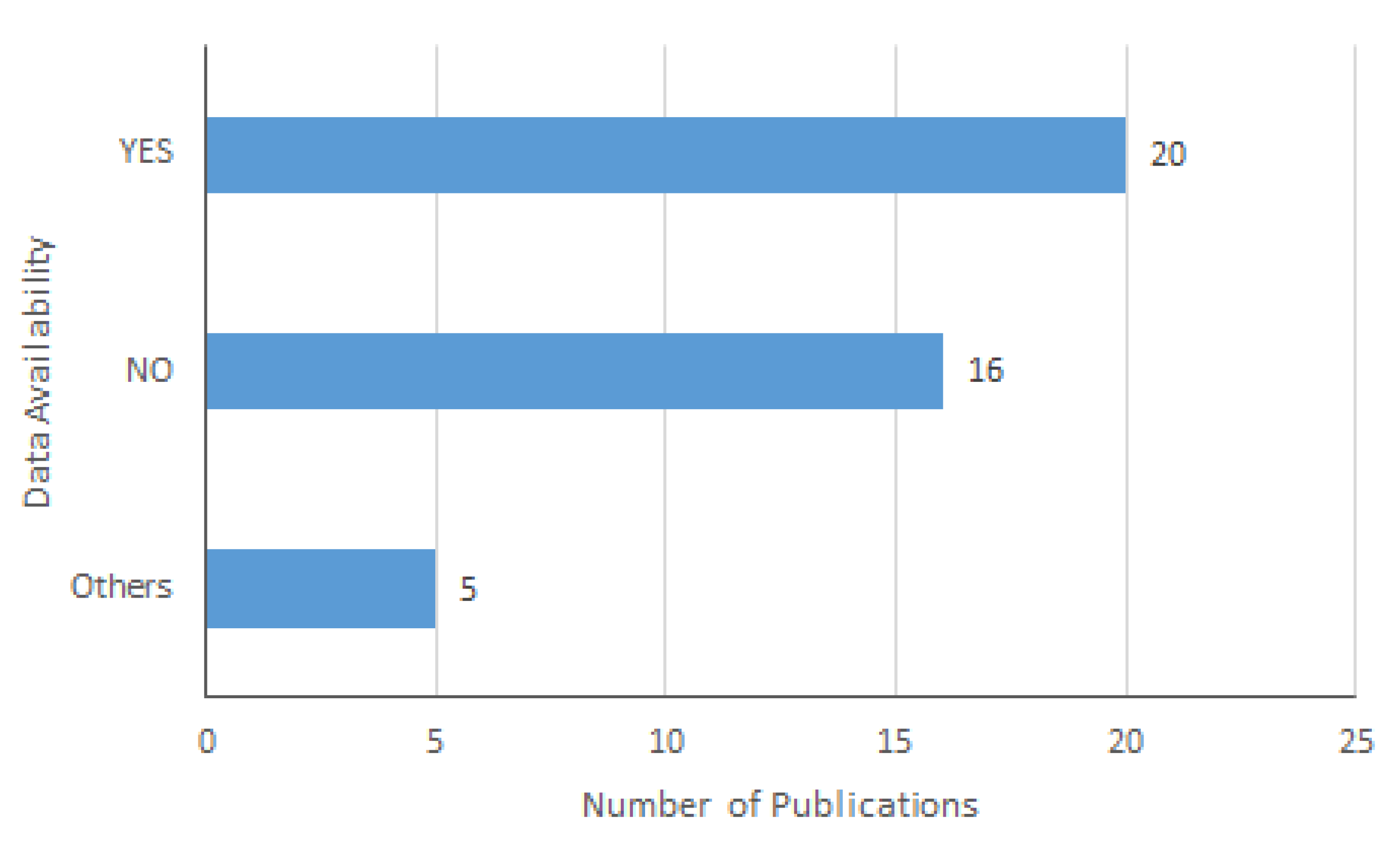
[12]	AQ, MET		YES	mRMR is preferable for future selection.		Longer term is not satisfactory, long time consuming on optimal subset selection and the model optimization.
[13]	AQ, Spatial		NO	IDW helped to improve BLSTM by 5.6%.		Using only the historic air pollution data.
[52]	AQ, MET, WFD, Spatial		NO	Faster training rate, higher accuracy.		$N/S$
[14]	AQ, MET		YES	To obtain a sequence pattern.		$N/S$
[39]	AQ, MET		NO	RFR reduces overfitting, detects peak values.		To use additional factors related to the air pollution.
[61]	AQ, MET		YES	Relatively better result, time complexity is linear.		To use more than three classifiers and remove classifiers with negative weight.
[17]	AQ, MET		ON REQUEST	Reduction of error addition and the training time.		To work on spatial attention, to collect more weather forecast data
[63]	AQ, MET		NO	Comparatively better accuracy.		It fails to consider the potential factors in extreme conditions, additional extension—to achieve medium- and long-term forecasts in terms of time factor.
[54]	AQ, MET		YES	The models’ computation time for real-time hourly prediction is less compared to the station-specific machine learning models.		high-ozone episodes were underpredicted, particularly during the high-ozone season.
[18]	AQ, MET		YES	AIS-RNN outperformed the baselines by up to 38%.		To extend AIS-RNN as an end-to-end ensemble mode.
[65]	AQ		YES	$N/S$		$N/S$
[40]	AQ, MET		NO	80% ≤ R2 ≤ 90%, O3 < 11 $\mathsf{\mu }$g/m${}^3$.		To consider and analyse new elements, to transfer information to the target groups.
[67]	AQ, MET		YES	To improve the convergence of optimization and to speed up the training process for big data.		Consider the commonalities between nearby meteorology stations.
[53]	AQ, MET, Temporal		YES	Better for Short-term and severe air pollution prediction.		More exploration must be done.
[16]	AQ, MET		YES	Relatively better result.		$N/S$
[20]	AQ, MET		NO	High stability and robustness.		Difficulties to make WNN.
[21]	AQ, MET		YES	Correlation result is 18% better, while the MAE declines by 15.7 $\mathsf{\mu }$g/m${}^3$.		The lack of data.
[22]	AQ, MET, WFD		NO	2.4%, 12.2%, 63.2% relative accuracy improvements on short-term, long-term and sudden changes prediction, respectively.		The long-term sudden changes prediction.
[64]	AQ, MET		YES	Higher applicability and effectiveness.		To forecast other air pollution indexes, to evaluate the AQ in other cities.
[55]	AQ, WFD, Spatial		NO	Effective and reaches nearly 60% in accuracy.		$N/S$
Work	Year	Case Study	Methods	Algorithms	Evaluation Metrics	Prediction Target	Time Granularity	Data Rates
[68]	2017	Iran	Multinomial Naïve Bayes and Multinomial Logistic Regression		Precision, Recall, F1 score	$N/S$	24 h	Hourly
[66]	2017	China	CEEMD-VMD-DE-ELM	Hybrid model	MAE, MAPE, RMSE	$N/S$	24 h	Daily
[56]	2017	China	MELSA	Ensemble	RAE, RSE, R	PM2.5, PM10, SO2, CO, NOx, O3	72 h	$N/S$
[41]	2017	Egypt	chWSVR	Regression	RMSE, R, z’, t-value	PM10	1 h	Hourly
[29]	2017	China	ELM	NN	MAE, RMSE, IA, R2	NO2, NOx, O3, PM2.5, SO2	24 h	Daily
[30]	2017	China	MSA-BPNN-ARIMA	NN	RMSE	PM2.5	24 h	Hourly
[42]	2017	USA	nu-SVM	Regression	R2	BC	24 h	Daily
[31]	2017	Italy	DNN	NN	AVG, SD, MIN, MAX	CO, NO2, NOx, C6H6, NMHC	$N/S$	Hourly
[33]	2016	China	STELM	NN	MRE, MAE	PM2.5	72 h	Hourly
[45]	2016	Romania	M5P, REPTree	Regression	R, MAE, RMSE	PM10	24 h, 48 h, 72 h	Daily
[34]	2016	Qatar	SVM, ANN, M5P	Regression, NN	PTA, RMSE, NRMSE	O3, NO2, SO2	1 h, 8 h, 12 h, 24 h	15 min
[46]	2016	Spain	LR, QR, IBKreg, M5P, RF	Regression, Ensemble	RMSE	SO2, O3, NO, NO2	3 h	Hourly
[35]	2016	Finland	ELM	NN	$N/S$	$N/S$	1 h	Hourly
[59]	2015	China	RF, GB, SVM	Ensemble	$N/S$	$N/S$	24 h	Daily
[60]	2014		DRR	Ensemble	RMSE	O3, NO2, PM10	24 h, 48 h, 72 h	Hourly
[36]	2014	China	ELM	NN	$N/S$	PM10	24 h	Daily
[48]	2014	Saudi Arabia	MLR, QR, GAM, BRT1, BRT2	Regression	MBE, MAE, RMSE, FACT2, R, IA	PM10	1 h	Hourly
[49]	2010	China	LSSVM	Regression	Relative Error	SPM, SO2, NO2, O3	24 h	Daily
[50]	2008	China	online SVM	Regression	MAE, RMSE, WIA	RSP(PM10), NOx, SO2	24 h, 1 week	Hourly
[38]	2003	China	ARBF/ARBF-PCA/SVM	NN	MAE, RMSE, WIA	RSP (PM10)	72 h	Hourly
[51]	2002	China	SVM	Regression	MAE	RSP(PM10)	24 h, 1 week	Hourly
Work	Dataset Type		Dataset Type	Advantages		Limitation/Future Work
[68]	AQ, MET		NO	$N/S$		To use SVM, DT and hybrid algorithms to improve the accuracy in existence of imbalanced datasets, to use spatial indexing method.
[66]	AQ		YES	To eliminate the non-stationary characteristics		$N/S$
[56]	AQ, MET, WFD		YES	$N/S$		$N/S$
[41]	AQ, MET, Temporal		NO	$N/S$		To forecast other air pollutants.
[29]	AQ, MET, Temporal		NO	Precision, robustness, generalization		$N/S$
[30]	AQ, MET, Social Media		NO	$N/S$		Long-term prediction is a challenging task
[42]	AQ, MET, Spatial, Temporal		Partially	$N/S$		Lack of monitors.
[31]	AQ, MET		YES	$N/S$		To extend the algorithm, to include more parameters.
[33]	AQ, MET, Spatial		NO	$N/S$		To improve the precision and reduce the absolute errors.
[45]	AQ, MET		YES	$N/S$		$N/S$
[34]	AQ, MET, Temporal		NO	M5P outperforms others because of the tree structure efficiency and powerful generalization ability.		To consider data changes over time for real-time forecasting. For increasing data seasonality to include more data.
[46]	AQ, MET, TIF, Temporal		YES	$N/S$		To include local features of the target points.
[35]	AQ, MET		YES	The method is flexible and reliable.		To use ensemble methods.
[59]	AQ, WFD, Chemical		Link is not available	Combined model outperforms single model by 3%.		$N/S$
[60]	AQ, MET		YES	$N/S$		$N/S$
[36]	AQ, MET		YES	The short training time, the small model size and managing imbalance dataset.		To compare different imbalance strategies.
[48]	AQ, MET		NO	QRM captures the contributions of covariates at different quantiles.		To use data from different monitoring sites over a longer period of time, to include traffic characteristics data.
[49]	AQ, MET		YES	$N/S$		$N/S$
[50]	AQ, MET		NO	Online SVM determine dynamically the optimal prediction model.		Computational problem because of dimensionality.
[38]	AQ, MET		NO	$N/S$		To provide more effective and practical models.
[51]	AQ, MET		NO	SVM is better than RBF.		To impove SVM method.

). Table 2 includes Year, Case Study, Methods, Algorithms, Evaluation Metrics, Prediction Target, Time Granularity, Data Rates, Dataset Types, Open Data, Advantages and Limitation/Future Work.

Year: as we have already seen (Section 3.1), Figure 2 displays the evolution of the publications over the years. We can see a significant increase since 2014–2015, which can be explained with the appearance of smart cities and open data portals notions in science.

Algorithms: having information about the distribution of the publications per each machine learning algorithm (Figure 4), it would be interesting to know how the usage of the algorithms changed throughout the years. Figure 5 presents the publications for each machine learning algorithm over the years. It can be noted that, in recent years, the number of publications (used neural network, ensemble and hybrid models) has an increasing trend, which is not applicable to the regression method. The latter one has been applied since 2002 almost with the unchangeable trend, moreover, in recent publications, the regression method was mainly applied along with other algorithms for comparison purposes.

Evaluation Metrics: are the metrics used in order to measure applied methods. Figure 6 displays for each metric the number of publications where the metric was applied. We can notice that the most used metrics are RMSE (Equation (1)) and MAE (Equation (2)), each of them applied in 24 publications.

$$RMSE={\left(\frac{1}{n}\sum _{i=1}^n{(E_i-A_i)}^2\right)}^{1/2}$$

(1)

$$MAE=\frac{1}{n}\sum _{i=1}^n|E_i-A_i|$$

(2)

where n is the number of instances, $E_i$ and $A_i$ are the estimated and actual values. The lower value of these two metrics corresponds to a better prediction.

Prediction Target: is the main pollutant in the case study, for which prediction different techniques were applied in order to monitor, to measure, and in the final step, to predict the concentration of that pollutant. Figure 7 represents the pollutants which were considered as a prediction target in the selected studies. The targets are PM_2.5, NO_x, O₃, PM₁₀ which in early publications was mentioned as RSP, SO₂, CO, Suspended Particulate Matter (SPM), NMHC, C₆H₆, black carbon (BC), and $N/S$ is the number of publications that did not specify the prediction target. It can be noted that PM_2.5 is the principal pollutant, being as the prediction target in 19 studies.

In general, the prediction of particulate matters has always been the main focus of researchers. The only significant change over the years is the ability to measure and monitor finer particulate matters with the help of new sensors (Figure 8).

After finding out the main pollutant of the selected papers, it is interesting to explore countries distribution per pollutant. In Figure 9, we can see that the case study of 18 publications out of 19, having PM_2.5 as a pollutant target, is China.

Time Granularity: is time resolution which is considered as the prediction interval. In Figure 10, we can notice that most used time resolutions were 24 h in 17 papers, and just in four papers the authors tried to make weekly prediction. The main reason is the issue related to the accuracy of long term predictions (for example, in [12] RMSE for the next 1h was 9.3953, for the next 5 h it was 37.6874 and for the next 10 h it was 65.7108).

Data Rates: is a frequency of the data acquisition from the sensors. Figure 11 presents data obtainment frequency for the selected studies. As it might be seen, in the majority of the papers (27) sensors provided hourly data, in nine studies sensors provide daily data, in one paper the frequency was 15 min, and the rest includes publications which did not provide any information about data rates.

Dataset Types: include types of data which were used in order to perform analysis. The used dataset types involve AQ: air quality data, MET: meteorological data, Temporal: include the day of the month (values from 1 to 31), day of the week (values from 1 to 7), the hour of the day (values from 1 to 24), WFD: weather forecast data, Spatial: in one paper it refers to proximity to transportation, topographical characteristics, neighbourhood characteristics, and for the rest cases it indicates the locations of the stations, Social Media: microblog data, Chemical: chemical component forecast data (organic carbon, black carbon, sea salt, etc.) and TIF: traffic intensity features, which contains information about traffic level in the surrounding stations (vehicles/hour). As shown in Figure 12, in the majority of the papers (36) air quality data was combined with meteorological data, considering the importance of the latter one in air quality prediction. The next types are temporal data in six papers, weather forecast data in five papers, spatial data in five papers, and social media, chemical forecast data, traffic intensity features, each of them in one paper.

Open Data: includes information about data accessibility. Taking into consideration the role of reproducibility nowadays, we explored to know which papers provide a link to the dataset used to carry out the experiments. However, it is worth mentioning that reproducibility is not only data; it also refers to code availability [69]. No paper provided code scripts, although the algorithms were available and were explained in the papers. Figure 13 shows data accessibility of the selected studies. We can see that 20 papers for their analysis used open data, 16 papers used private data, and Others includes five papers; in the first paper the authors mentioned that data can be available through the request, the second paper used partially available data, the third study provided link to access to the data, but now the link is not available, and the other two studies mentioned that they took data from Hong Kong Environmental Protection Department without providing any reference. Figure 14 displays the number of publications for data accessibility over the years. We can notice that since 2010 the authors have started to use open data portals to capture data to perform analysis and since 2017, in contrast to papers using private data, the number of publications having open data increased.

Advantages: are the main findings of the methods which can improve the accuracy of the prediction. Here are several findings extracted from the studies. According to Xu and Ren [12] ESN and ELM consume less time to train data than the deep learning model. Compared to the random forest, correlation feature selection, fast correlation-based filter, mutual information, information gain, regularization models, relief-based algorithms, and genetic algorithm, mRMR is preferable for future selection. Ma et al. [13] mentioned that LSTM based algorithms performed better than RNN, and because of bidirectional modelling concept BLSTM provided better results compared to LSTM, integration of IDW improved BLSTM by 5.6% because the spatial factor was taken into consideration. Zhang et al. [52] pointed out the advantage of LightGBM, being a histogram-based algorithm, processes high-dimensional big data better compared to the other boost algorithms. Tao et al. [14] also mentioned the superiority of LSTM compared to RNN and confirmed the advantage of the bidirectional model. According to Ameer et al. [39] compared to a decision tree, gradient boosting and multilinear perception, random forest obtained better results by reducing overfitting and detecting peak values. Although, on the other hand, Li and Ngan [61] mentioned that random forest could have a challenge with fitting a wide variety of data distribution. Shaban et al. [34] noted that M5P compared to SVM and ANN, generalised better, and SVM can manage high dimensional data better than ANN.

Limitation/Future work: are the main reasons that authors considered as a challenge for obtaining higher accuracy. Some authors mentioned limitation, some of them propose to expand the work applying certain mechanism. It can be noticed that in many studies as a limitation was mentioned the lack of the data (also considering data types).

After finding out that the most used metric are MAE and RMSE, the most used time granularity is 24 h, and the most used prediction target is PM_2.5, we have decided to extract the accuracy from the papers which predicted PM_2.5 for the next 24 h and which measured the accuracy using MAE and RMSE in order to compare machine learning algorithms (

Table 3. PM_2.5 prediction accuracy for the next 24 h measured by mean absolute error (MAE) and root mean square error (RMSE). $N/S$: Not Specified.

Work	Algorithms	MAE_24h	RMSE_24h
[13]	NN	8.49	12.03
[17]	NN	34.35	$N/S$
[22]	NN	45.1±0.1	$N/S$
[29]	NN	5.5	6.9
[30]	NN	$N/S$	24.06
[52]	Ensemble	26.44	$N/S$
[55]	Ensemble	34.25	$N/S$
[67]	$N/S$	$N/S$	0.03

). Table 3 shows the output after the extraction process. It can be seen that there are not many papers matching our criteria, which created some difficulties to complete our comparison. For MAE_24h we have papers applying neural networks and ensemble algorithms, and for RMSE_24h the papers used neural networks, and one paper used regularization and optimization. Looking at the values, we can notice that there is a significant difference between neural networks and regularization-optimization (the latter one has quite a high accuracy: 0.03), which is not applicable to MAE_24h. Overall, because of the lack of information, it is challenging to compare the accuracy of machine learning algorithms.

5. Conclusions

The objective of this paper is to give a general perception of the current approaches presented related to the air quality prediction concept by reviewing the recent publications. As air quality prediction is a huge topic, we have defined a set of key points in order to narrow the scope and focus on a specific task. To select papers, we inserted a beforehand defined query in the following databases: Scopus and IEEE Xplore repositories. For further observation, we have selected studies published since 2002 and, afterwards, by excluding irrelevant papers based on the inclusion/exclusion criteria. Eventually, 41 manuscripts were selected. Reviewing the chosen papers, we have extracted the essential features and based on the latter findings, the papers were linked, and further comparison was carried out.

Taking into consideration the geographical component, the result shows that China was the leading country being the case study in 26 papers. The important finding was that to increase the accuracy of air quality prediction, it is valuable, in addition to the air quality data, to include also a dataset of other factors that affects the air quality. Thus, in most cases, the authors used meteorological data, and some of them also involved other types of data, such as calendar features, traffic intensity features, spatial features, etc.

Related to the prediction target, the outcome shows that PM_2.5 was the main element, applied in 19 papers, 18 of which utilised data of the cities located in China. Most cases, the authors performed a prediction for the next day. Twenty-seven studies used data hourly collected from the sensors.

Among the analysed works, 20 of them use open data to perform air quality predictions. These works were carried out from 2014 until now, coinciding with the movement of open data within the cities [70]. Therefore, we can affirm that the open data movement has increased the number of research works in the field of machine learning, especially in the prediction of air quality.

Regarding machine learning techniques, the studies used neural networks (38%), regression(24%), ensemble (22%), hybrid (11%) models, one study used regularization and optimization, and the other research applied multinomial naïve bayes and multinomial logistic regression methods. For evaluating applied techniques tailored to the algorithms mentioned above, different metrics were applied. Overall, 29 metrics were applied, from which MAE and RMSE were the most used metrics, each of them being applied in 24 papers. It is very important to mention the challenges regarding the data. First of all, for an accurate air quality prediction it is essential to capture as much relevant data as possible, including weather forecast data, air quality data, meteorological data, etc. Then, it is necessary to apply different techniques (e.g., PCA) to remove redundant data and to select representative subsets for further analysis. It is also important to mention that air quality prediction for a long temporal resolution is a challenging task, as the accuracy decreases with the increase of the prediction interval. Another essential aspect is time complexity; for example, methods based on neural network algorithms to train data, usually require a long time.

In general, it is very difficult to compare the results obtained during analysis of the papers, as they used different data, and they analysed different temporal granularity. As future work, an exhaustive work is proposed. Using all the suggested methods, they should be developed and tested using the same datasets. In this way, the results could be compared in a similar and fair scale.

References

- Urban Population (% of Total Population). Available online: https://data.worldbank.org/indicator/SP.URB.TOTL.IN.ZS?name_desc=false (accessed on 13 March 2020).
- Urban Population Change. Available online: https://www.un.org/development/desa/en/news/population/2018-revision-of-world-urbanization-prospects.html. (accessed on 13 March 2020).
- Giffinger, R.; Fertner, C.; Kramar, H.; Kalasek, R.; Pichler-Milanović, N.; Meijers, E. Smart cities: Ranking of european medium-sized cities. vienna, austria: Centre of regional science (srf), vienna university of technology. Available online: http://www.smart-cities.eu/download/smart_cities_final_report.pdf (accessed on 31 March 2020).
- Wan, J.; Li, D.; Zou, C.; Zhou, K. M2M communications for smart city: An event-based architecture. In Proceedings of the 2012 IEEE 12th International Conference on Computer and Information Technology, Chengdu, China, 27–29 October 2012; pp. 895–900. [Google Scholar]
- Trilles, S.; Calia, A.; Belmonte, Ó.; Torres-Sospedra, J.; Montoliu, R.; Huerta, J. Deployment of an open sensorized platform in a smart city context. Future Gener. Comput. Syst. 2017, 76, 221–233. [Google Scholar] [CrossRef]
- Granell, C.; Kamilaris, A.; Kotsev, A.; Ostermann, F.O.; Trilles, S. Internet of Things. In Manual of Digital Earth; Springer: Singapore, 2020; pp. 387–423. [Google Scholar]
- Air Pollution. Available online: https://www.who.int/health-topics/air-pollution#tab=tab_1/ (accessed on 13 March 2020).
- Apte, J.S.; Brauer, M.; Cohen, A.J.; Ezzati, M.; Pope, C.A., III. Ambient PM2.5 reduces global and regional life expectancy. Environ. Sci. Technol. Lett. 2018, 5, 546–551. [Google Scholar] [CrossRef] [Green Version]
- Cohen, A.J.; Ross Anderson, H.; Ostro, B.; Pandey, K.D.; Krzyzanowski, M.; Künzli, N.; Gutschmidt, K.; Pope, A.; Romieu, I.; Samet, J.M.; et al. The global burden of disease due to outdoor air pollution. J. Toxicol. Environ. Heal. Part 2005, 68, 1301–1307. [Google Scholar] [CrossRef] [PubMed]
- Cohen, A.J.; Brauer, M.; Burnett, R.; Anderson, H.R.; Frostad, J.; Estep, K.; Balakrishnan, K.; Brunekreef, B.; Dandona, L.; Dandona, R.; et al. Estimates and 25-year trends of the global burden of disease attributable to ambient air pollution: an analysis of data from the Global Burden of Diseases Study 2015. Lancet 2017, 389, 1907–1918. [Google Scholar] [CrossRef] [Green Version]
- Rybarczyk, Y.; Zalakeviciute, R. Machine learning approaches for outdoor air quality modelling: A systematic review. Appl. Sci. 2018, 8, 2570. [Google Scholar] [CrossRef] [Green Version]
- Xu, X.; Ren, W. Prediction of Air Pollution Concentration Based on mRMR and Echo State Network. Appl. Sci. 2019, 9, 1811. [Google Scholar] [CrossRef] [Green Version]
- Ma, J.; Ding, Y.; Gan, V.J.; Lin, C.; Wan, Z. Spatiotemporal Prediction of PM2.5 Concentrations at Different Time Granularities Using IDW-BLSTM. IEEE Access 2019, 7, 107897–107907. [Google Scholar] [CrossRef]
- Tao, Q.; Liu, F.; Li, Y.; Sidorov, D. Air Pollution Forecasting Using a Deep Learning Model Based on 1D Convnets and Bidirectional GRU. IEEE Access 2019, 7, 76690–76698. [Google Scholar] [CrossRef]
- Liang, X.; Zou, T.; Guo, B.; Li, S.; Zhang, H.; Zhang, S.; Huang, H.; Chen, S.X. Assessing Beijing’s PM2.5 pollution: severity, weather impact, APEC and winter heating. Proc. R. Soc. Math. Phys. Eng. Sci. 2015, 471, 20150257. [Google Scholar] [CrossRef] [Green Version]
- Huang, C.J.; Kuo, P.H. A deep cnn-lstm model for particulate matter (PM2.5) forecasting in smart cities. Sensors 2018, 18, 2220. [Google Scholar] [CrossRef] [Green Version]
- Liu, B.; Yan, S.; Li, J.; Qu, G.; Li, Y.; Lang, J.; Gu, R. A Sequence-to-Sequence Air Quality Predictor Based on the n-Step Recurrent Prediction. IEEE Access 2019, 7, 43331–43345. [Google Scholar] [CrossRef]
- Munkhdalai, L.; Munkhdalai, T.; Park, K.H.; Amarbayasgalan, T.; Erdenebaatar, E.; Park, H.W.; Ryu, K.H. An End-to-End Adaptive Input Selection with Dynamic Weights for Forecasting Multivariate Time Series. IEEE Access 2019, 7, 99099–99114. [Google Scholar] [CrossRef]
- UCI Machine Learning Repository. Available online: https://archive.ics.uci.edu/ml/index.php (accessed on 13 March 2020).
- Zhang, S.; Li, X.; Li, Y.; Mei, J. Prediction of Urban PM 2.5 Concentration Based on Wavelet Neural Network. In Proceedings of the 2018 Chinese Control And Decision Conference (CCDC), Shenyang, China, 9–11 June 2018; pp. 5514–5519. [Google Scholar]
- Lu, H.; Song, J.; Di, T.; Kurdestany, J.M.; Wang, H. A deep belief network based model for urban haze prediction. Teh. ki vjesnik 2018, 25, 519–527. [Google Scholar]
- Yi, X.; Zhang, J.; Wang, Z.; Li, T.; Zheng, Y. Deep distributed fusion network for air quality prediction. In Proceedings of the 24th ACM SIGKDD International Conference on Knowledge Discovery & Data Mining, London, UK, 19–23 August 2018; pp. 965–973. [Google Scholar]
- Zheng, Y.; Yi, X.; Li, M.; Li, R.; Shan, Z.; Chang, E.; Li, T. Forecasting fine-grained air quality based on big data. In Proceedings of the 21th ACM SIGKDD International Conference on Knowledge Discovery and Data Mining, Sydney, Australia, 10–13 August 2015; pp. 2267–2276. [Google Scholar]
- Zhang, J.; Zheng, Y.; Qi, D.; Li, R.; Yi, X. DNN-based prediction model for spatio-temporal data. In Proceedings of the 24th ACM SIGSPATIAL International Conference on Advances in Geographic Information Systems, Burlingame, CA, USA, 31 October–3 November 2016; pp. 1–4. [Google Scholar]
- Yao, H.; Wu, F.; Ke, J.; Tang, X.; Jia, Y.; Lu, S.; Gong, P.; Ye, J.; Li, Z. Deep multi-view spatial-temporal network for taxi demand prediction. In Proceedings of the Thirty-Second AAAI Conference on Artificial Intelligence, New Orleans, LO, USA, 2–7 February 2018. [Google Scholar]
- Kingma, D.P.; Ba, J. Adam: A method for stochastic optimization. arXiv 2014, arXiv:1412.6980. [Google Scholar]
- Guo, H.; Tang, R.; Ye, Y.; Li, Z.; He, X. DeepFM: a factorization-machine based neural network for CTR prediction. arXiv 2017, arXiv:1703.04247. [Google Scholar]
- A Weather-Forecast-Based Prediction Method. Available online: http://zx.bjmemc.com.cn/ (accessed on 13 March 2020).
- Zhang, J.; Ding, W. Prediction of air pollutants concentration based on an extreme learning machine: the case of Hong Kong. Int. J. Environ. Res. Public Health 2017, 14, 114. [Google Scholar] [CrossRef]
- Ni, X.; Huang, H.; Du, W. Relevance analysis and short-term prediction of PM2.5 concentrations in Beijing based on multi-source data. Atmos. Environ. 2017, 150, 146–161. [Google Scholar] [CrossRef]
- Vidnerova, P.; Neruda, R. Evolving keras architectures for sensor data analysis. In Proceedings of the 2017 Federated Conference on Computer Science and Information Systems (FedCSIS), Prague, Czech Republic, 3–6 September 2017; pp. 109–112. [Google Scholar]
- Keras. Available online: https://github.com/keras-team/keras (accessed on 13 March 2020).
- Liu, B.; Yan, S.; Li, J.; Li, Y. Forecasting PM2.5 concentration using spatio-temporal extreme learning machine. In Proceedings of the 2016 15th IEEE International Conference on Machine Learning and Applications (ICMLA), Anaheim, CA, USA, 18–20 December 2016; pp. 950–953. [Google Scholar]
- Shaban, K.B.; Kadri, A.; Rezk, E. Urban air pollution monitoring system with forecasting models. IEEE Sens. J. 2016, 16, 2598–2606. [Google Scholar] [CrossRef]
- Zhao, C.; van Heeswijk, M.; Karhunen, J. Air quality forecasting using neural networks. In Proceedings of the 2016 IEEE Symposium Series on Computational Intelligence (SSCI), Athens, Greece, 6–9 December 2016; pp. 1–7. [Google Scholar]
- Vong, C.M.; Ip, W.F.; Wong, P.K.; Chiu, C.C. Predicting minority class for suspended particulate matters level by extreme learning machine. Neurocomputing 2014, 128, 136–144. [Google Scholar] [CrossRef]
- Macau Government Meteorological Center. Available online: http://www.smg.gov.mo/www/ccaa/pdf/e_pdf_download.php (accessed on 9 May 2012).
- Wang, W.; Xu, Z.; Lu, J.W. Three improved neural network models for air quality forecasting. Eng. Comput. 2003, 20, 192–210. [Google Scholar] [CrossRef] [Green Version]
- Ameer, S.; Shah, M.A.; Khan, A.; Song, H.; Maple, C.; Islam, S.U.; Asghar, M.N. Comparative Analysis of Machine Learning Techniques for Predicting Air Quality in Smart Cities. IEEE Access 2019, 7, 128325–128338. [Google Scholar] [CrossRef]
- Martínez-España, R.; Bueno-Crespo, A.; Timon-Perez, I.M.; Soto, J.; Muñoz, A.; Cecilia, J.M. Air-Pollution Prediction in Smart Cities through Machine Learning Methods: A Case of Study in Murcia, Spain. J. UCS 2018, 24, 261–276. [Google Scholar]
- Eldakhly, N.M.; Aboul-Ela, M.; Abdalla, A. Air pollution forecasting model based on chance theory and intelligent techniques. Int. J. Artif. Intell. Tools 2017, 26, 1750024. [Google Scholar] [CrossRef]
- Awad, Y.A.; Koutrakis, P.; Coull, B.A.; Schwartz, J. A spatio-temporal prediction model based on support vector machine regression: Ambient Black Carbon in three New England States. Environ. Res. 2017, 159, 427–434. [Google Scholar] [CrossRef] [PubMed]
- Allen, G. Analysis of Spatial and Temporal Trends of Black Carbon in Boston; Technical Report for Northeast States for Coordinated Air Use Management: New York, NY, USA, 2014. [Google Scholar]
- IMPROVE. Available online: http://vista.cira.colostate.edu/improve/ (accessed on 13 March 2020).
- Oprea, M.; Dragomir, E.G.; Popescu, M.; Mihalache, S.F. Particulate matter air pollutants forecasting using inductive learning approach. Rev. Chim. 2016, 67, 2075–2081. [Google Scholar]
- Contreras, L.; Ferri, C. Wind-sensitive interpolation of urban air pollution forecasts. Procedia Comput. Sci. 2016, 80, 313–323. [Google Scholar] [CrossRef] [Green Version]
- AEMET. Available online: http://www.aemet.es/es/portada (accessed on 13 March 2020).
- Sayegh, A.S.; Munir, S.; Habeebullah, T.M. Comparing the performance of statistical models for predicting PM10 concentrations. Aerosol Air Qual. Res. 2014, 14, 653–665. [Google Scholar] [CrossRef] [Green Version]
- Ip, W.F.; Vong, C.M.; Yang, J.; Wong, P. Forecasting daily ambient air pollution based on least squares support vector machines. In Proceedings of the 2010 IEEE International Conference on Information and Automation, Harbin, China, 20–23 June 2010; pp. 571–575. [Google Scholar]
- Wang, W.; Men, C.; Lu, W. Online prediction model based on support vector machine. Neurocomputing 2008, 71, 550–558. [Google Scholar] [CrossRef]
- Lu, W.; Wang, W.; Leung, A.Y.; Lo, S.M.; Yuen, R.K.; Xu, Z.; Fan, H. Air pollutant parameter forecasting using support vector machines. In Proceedings of the 2002 International Joint Conference on Neural Networks—IJCNN’02 (Cat. No. 02CH37290), Honolulu, HI, USA, 12–17 May 2002; Volume 1, pp. 630–635. [Google Scholar]
- Zhang, Y.; Wang, Y.; Gao, M.; Ma, Q.; Zhao, J.; Zhang, R.; Wang, Q.; Huang, L. A predictive data feature exploration-based air quality prediction approach. IEEE Access 2019, 7, 30732–30743. [Google Scholar] [CrossRef]
- Zheng, H.; Li, H.; Lu, X.; Ruan, T. A multiple kernel learning approach for air quality prediction. Adv. Meteorol. 2018, 2018, 3506394. [Google Scholar] [CrossRef]
- Eslami, E.; Salman, A.K.; Choi, Y.; Sayeed, A.; Lops, Y. A data ensemble approach for real-time air quality forecasting using extremely randomized trees and deep neural networks. Neural Comput. Appl. 2019, 1–17. [Google Scholar] [CrossRef]
- Wang, J.; Song, G. A deep spatial-temporal ensemble model for air quality prediction. Neurocomputing 2018, 314, 198–206. [Google Scholar] [CrossRef]
- Zhang, C.; Yan, J.; Li, Y.; Sun, F.; Yan, J.; Zhang, D.; Rui, X.; Bie, R. Early air pollution forecasting as a service: An ensemble learning approach. In Proceedings of the 2017 IEEE International Conference on Web Services (ICWS), Honolulu, HI, USA, 25–30 June 2017; pp. 636–643. [Google Scholar]
- Grell, G.A.; Peckham, S.E.; Schmitz, R.; McKeen, S.A.; Frost, G.; Skamarock, W.C.; Eder, B. Fully coupled “online” chemistry within the WRF model. Atmos. Environ. 2005, 39, 6957–6975. [Google Scholar] [CrossRef]
- Karamchandani, P.; Johnson, J.; Yarwood, G.; Knipping, E. Implementation and application of sub-grid-scale plume treatment in the latest version of EPA’s third-generation air quality model, CMAQ 5.01. J. Air Waste Manag. Assoc. 2014, 64, 453–467. [Google Scholar] [CrossRef] [PubMed] [Green Version]
- Xi, X.; Wei, Z.; Xiaoguang, R.; Yijie, W.; Xinxin, B.; Wenjun, Y.; Jin, D. A comprehensive evaluation of air pollution prediction improvement by a machine learning method. In Proceedings of the 2015 IEEE International Conference on Service Operations and Logistics, And Informatics (SOLI), Hammamet, Tunisia, 15–17 November 2015; pp. 176–181. [Google Scholar]
- Debry, E.; Mallet, V. Ensemble forecasting with machine learning algorithms for ozone, nitrogen dioxide and PM10 on the Prev’Air platform. Atmos. Environ. 2014, 91, 71–84. [Google Scholar] [CrossRef]
- Li, L.; Ngan, C.K. A Weight-adjusting Approach on an Ensemble of Classifiers for Time Series Forecasting. In Proceedings of the 2019 3rd International Conference on Information System and Data Mining, Houston, TX, USA, 6–8 April 2019; pp. 65–69. [Google Scholar]
- Air Quality Data Set. Available online: https://archive.ics.uci.edu/ml/datasets/Air+Quality (accessed on 13 March 2020).
- Xu, X.; Ren, W. Application of a Hybrid Model Based on Echo State Network and Improved Particle Swarm Optimization in PM2.5 Concentration Forecasting: A Case Study of Beijing, China. Sustainability 2019, 11, 3096. [Google Scholar] [CrossRef] [Green Version]
- Zhu, S.; Lian, X.; Wei, L.; Che, J.; Shen, X.; Yang, L.; Qiu, X.; Liu, X.; Gao, W.; Ren, X.; et al. PM2.5 forecasting using SVR with PSOGSA algorithm based on CEEMD, GRNN and GCA considering meteorological factors. Atmos Environ. 2018, 183, 20–32. [Google Scholar] [CrossRef]
- Wu, Q.; Lin, H. A novel optimal-hybrid model for daily air quality index prediction considering air pollutant factors. Sci. Total. Environ. 2019, 683, 808–821. [Google Scholar] [CrossRef]
- Wang, D.; Wei, S.; Luo, H.; Yue, C.; Grunder, O. A novel hybrid model for air quality index forecasting based on two-phase decomposition technique and modified extreme learning machine. Sci. Total. Environ. 2017, 580, 719–733. [Google Scholar] [CrossRef]
- Zhu, D.; Cai, C.; Yang, T.; Zhou, X. A machine learning approach for air quality prediction: Model regularization and optimization. Big Data Cogn. Comput. 2018, 2, 5. [Google Scholar] [CrossRef] [Green Version]
- Asgari, M.; Farnaghi, M.; Ghaemi, Z. Predictive mapping of urban air pollution using Apache Spark on a Hadoop cluster. In Proceedings of the 2017 International Conference on Cloud and Big Data Computing, London, UK, 17–19 September 2017; pp. 89–93. [Google Scholar]
- Zaragozí, B.M.; Trilles, S.; Navarro-Carrión, J.T. Leveraging Container Technologies in a GIScience Project: A Perspective from Open Reproducible Research. ISPRS Int. J. Geo-Inf. 2020, 9, 138. [Google Scholar] [CrossRef] [Green Version]
- Degbelo, A.; Granell, C.; Trilles, S.; Bhattacharya, D.; Casteleyn, S.; Kray, C. Opening up smart cities: citizen-centric challenges and opportunities from GIScience. ISPRS Int. J. Geo-Inf. 2016, 5, 16. [Google Scholar] [CrossRef] [Green Version]