Featured Application
Speech enhancement; speech recognition; music information retrieval.
Abstract
Single-channel singing voice separation has been considered a difficult task, as it requires predicting two different audio sources independently from mixed vocal and instrument sounds recorded by a single microphone. We propose a new singing voice separation approach based on the curriculum learning framework, in which learning is started with only easy examples and then task difficulty is gradually increased. In this study, we regard the data providing obviously dominant characteristics of a single source as an easy case and the other data as a difficult case. To quantify the dominance property between two sources, we define a dominance factor that determines a difficulty level according to relative intensity between vocal sound and instrument sound. If a given data is determined to provide obviously dominant characteristics of a single source according to the factor, it is regarded as an easy case; otherwise, it belongs to a difficult case. Early stages in the learning focus on easy cases, thus allowing rapidly learning overall characteristics of each source. On the other hand, later stages handle difficult cases, allowing more careful and sophisticated learning. In experiments conducted on three song datasets, the proposed approach demonstrated superior performance compared to the conventional approaches.
1. Introduction
Single-channel singing voice separation aims to separate instrument sounds and vocal sounds from a given music data recorded by a single microphone. This problem has been considered as a difficult separation task in comparison with multi-channel signal separation that handles data recorded by two or more microphones. In recent years, deep neural network (DNN)-based modelling approaches such as convolutional neural network (CNN) [1,2,3], recurrent neural network (RNN) [4,5,6], and U-Net [7,8,9,10] have been adopted to overcome this difficulty. Although the conventional DNN-based approaches have reported improvement of separation performance, most of them have difficulties in obtaining a reliable convergence and they requires tremendous learning time. To overcome these limitations, we propose a new single-channel singing voice separation approach based on curriculum learning [11].
Curriculum learning is a type of learning method, in which learning is started with only easy examples and then task difficulty is gradually increased. Thus, it is capable of learning a model by gradually adjusting the difficulty of training data according to learning stages. Several successful applications of the curriculum learning include image classification [12], object detection [13,14], and optical flow estimation [15]. The difficulty level of the training data can be determined either by humans [14,15] or automatically [16]. The curriculum learning used in the proposed method is implemented by adjusting the weight of the loss function in RNN according to the relative dominance of one source to the other. Giving different weights according to the dominance allows reducing learning time, as the dominant data tend to converge rapidly to a vicinity of the dominant region. In addition, it can make sophisticated learning, as higher weights given to less dominant data lead to fine-tuning of the models. This paper is organized as follows—in Section 2, the conventional DNN-based singing voice separation approaches are addressed. Section 3 explains the proposed curriculum learning-based approach. In Section 4, several experimental results are described. And Section 5 concludes this paper.
2. Related Work
Figure 1 shows a typical framework of singing voice separation using a DNN [4,5,6]. First, the input mixture in the time-domain is transformed to magnitude and phase spectra using short-time Fourier transform (STFT). DNNs take the magnitude spectra of the mixed sound as input to obtain the spectral magnitudes of both vocal and instrument sounds. The inverse STFT is performed by combining the magnitude spectra predicted by the DNN model and the phase spectra of the input mixture to get separated vocals and musical instruments. Some types of DNNs for single-channel singing voice separation are convolutional neural networks (CNNs) [1,2,3], recurrent neural networks (RNNs) [4,5,6], convolutional recurrent neural networks (CRNNs) [17,18], and U-Net [7,8,9,10].
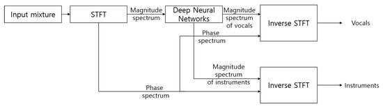
Figure 1.
Illustration of a typical deep neural network framework for singing voice separation. The input and output features are the magnitude spectra of the short-time Fourier transform (STFT) of the time-domain signals. Neural network models are applied to separate vocal and instrument sources in the magnitude STFT domain, and the audio sounds are reconstructed by inverse STFT operations.
2.1. RNN-Based Singing Voice Separation
RNN is a network created to process sequential data using memory, in other words, hidden states that are invisible to the outside of the network. A vanilla RNN conveying basic elements only is defined by the following equation:
where t is a discrete time index, is a hidden state output vector at time t, is an input vector whose components are magnitude spectra generated by STFT, is a bias vector, and g is an activation function. The input, state variable, and bias variable represented by boldface letters are all vectors. is a weight matrix from the past output () to the current output vectors (), and is another weight matrix from the input feature () to the output. RNN can process sequences of arbitrary length in such a way that hidden state summarizes the information of the previous inputs, , and combines them with the current input to calculate the output vector . According to the first Markovian assumption in Equation (1), the vanilla RNN assumes dependency to previous output only, so it may not be able to handle the cases where the dependency is complicated and exists over long time. To model multiple-level dependency in time, several vanilla RNNs are connected sequentially to build stacked RNNs as shown in Figure 2. Stacked RNN consists of several layers of multiple RNNs, and longer time dependencies are expected to be modeled by the cascaded recurrent paths.
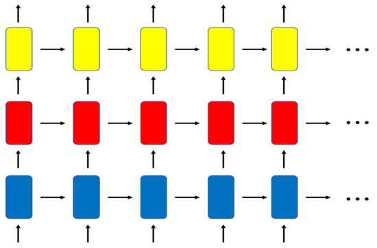
Figure 2.
Structure of stacked recurrent neural networks.
The dependency across both time and frequency axes can be modeled by convolutional neural networks (CNNs) [19,20]. The CNN architecture is not well suited to sequential data such as audio sounds because the size of its receptive field is fixed, and the convolution operation calculates the output based only on the region within the receptive field. However, CNN has its own advantage that most calculations can be implemented in a parallel manner, which, in terms of computational efficiency, makes a great advantage over RNN that requires computation of all previous outputs to be finalized before generating the current outputs. For these reasons, CNN and its variants [1,2,3] have been widely used for singing voice separation. In addition, there have been attempts to combine an RNN and a CNN. One of their combinations is a convolutional recurrent neural network (CRNN) that has been successfully adopted to singing voice separation as well [17,18].
2.2. Loss Function of Singing Voice Separation Models
To measure the error between the ground truth and the predicted spectra, there are many distance metrics which provide scale-invariance. One of such metrics for the STFT spectra is Itakura-Saito divergence [21], and it was applied to nonnegative matrix factorization (NMF) [22,23] with successful results in music sound analysis [22]. -divergence also provides scale-invariant distance, and it was applied to NMF as well [24,25]. However, in DNN learning, it is preferred to use simple metrics that are easy to differentiate to derive a learning algorithm and compute gradients efficiently. In our paper, we use mean squared error (MSE, squared L2 loss) between ground truth and predicted spectrum that was adopted to singing voice separation recently [7,8]. The MSE between two arbitrary STFT vectors and is defined as follows:
where f is a discrete frequency index, and F is the total number of frequency bins. The advantage of the squared L2 loss is that it is differentiable and has smoother convergence around 0. For the given ground truths in the powerspectral domain at time t, and , and their approximates, and , the prediction error is defined by the MSE averaged over all the frequency bins:
The objective function should be designed to reduce the prediction error between the ground truth and the approximate at all time and frequency units [4,5,6]:
where T is the number of samples in time. Learning using this loss is expected to yield a high signal to interference ratio (SIR) [26].
3. Proposed Curriculum Learning Technique on RNN and U-Net
In this section, the baseline models for the singing voice separation and the proposed curriculum learning framework are explained in detail, and the advantage of the proposed method is described. Our proposed method can be applied to various types of models that are based on stochastic learning. In this paper, we use a stacked RNN [4,5,6] and a U-Net [7] as reference baselines for the proposed method.
3.1. Stacked RNN-based Separation Model
Assume that is a STFT output obtained by a vector of dimension F at time t. In order to add temporal variation to the input feature vector, the previous and next frames are concatenated as follows:
The stacked RNN for the singing voice separation has three RNN layers followed by a fully connected (FC) layer as shown in Figure 3. The hidden state output at time t and level l, denoted by , is generated by passing the previous hidden state outputs, , through the RNN unit at level l, expressed as follows:
where is a sigmoid function, , , and are weight matrices and bias vector of the RNN at level l. The input to the RNN at level 1 is the mixed sounds described in Equation (5), that is, . The outputs of the last RNN layer pass through an FC layer with rectified linear unit (ReLU) activation function. At time t, the prediction of of source i is expressed as
where and are the weight matrix and the bias vector of the fully connected layer. Figure 3 illustrates the data flow of the stacked RNN. To train the weights, the objective function in Equation (4) is minimized with appropriate optimization method. Learning the stacked RNN is briefly summarized in Algorithm 1. Detailed derivation of the gradients can be found in Reference [4].
| Algorithm 1 Stacked RNN Learning |
|
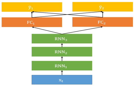
Figure 3.
Stacked RNN baseline architecture. Baseline model consists of three layers of multiple RNNs and a fully connected (FC) layer. Individual sources have their own FC layer, and the weight and bias parameters of RNN layers are shared.
Finally, the time frequency mask is obtained by using the ratio of the outputs of the individual FC layers, and . The magnitude spectrum vector of the separated sound is obtained by the element-wise multiplication of the time frequency mask and the spectrogram of the mixed input:
The original sound is reconstructed by inverse STFT on the magnitude and the phase components of the mixed sound.
3.2. U-Net Baseline Model
Our U-Net baseline model is based on Reference [7]. For the mixed input signals, STFT extracts magnitude spectrogram of size , where T is the number of frames in time domain and F is the number of frequency bins. Each component of the 2-dimensional matrix is a specific time-frequency unit region,
where t and f are discrete time and frequency index variables, and is STFT of the input mixture sound at time t and frequency f. The spectrogram matrix is globally scaled so that all the values of should be within for fast and stable learning. The encoder consists of six convolution layers with various kernel window sizes and stride values. Each convolution output is generated according to the following formula:
where g is an activation function, l is the layer number expressed by parenthesized superscripts, is a matrix whose column vectors are convolution kernel functions, and is a bias vector. The superscript and the subscript notations, , indicate that the parameter set belongs to layer l of the encoder network. The initial output is a copy of the input spectrogram, . The function “conv” defines a 2-dimensional convolution operator with the given set of a kernel matrix and a bias vector. The encoder extracts high-level features with resolution reduction from the input features.
Decoding part of the U-Net consists of five up-convolution layers with initial input as the encoder output at the final convolution layer. The outputs of the encoder layers are concatenated to the inputs of the decoding layers to compensate any lost information during encoding. The decoding operation from lower layer to the upper layer is recursively defined as follows:
where is a concatanetion operator, and are a matrix of the deconvolution kernel functions and a bias vector, and is an intermediate output at layer l. The initial input to the decoding up-convolution layer is the encoder output only, that is, . The detailed configuration including the sizes and the numbers of the kernel functions adopted in this paper is given in Table 1. Learning the U-Net baseline is briefly summarized in Algorithm 2. Exact calculation of the gradients can be found in Reference [7].
| Algorithm 2 U-Net Learning |
|

Table 1.
U-Net architecture for singing voice separation.
The activation function at the final layer is a sigmoid function, and its output bounded in is used as a mask for vocal sound. The size of the final output of the decoder, , is , and it is element-wisely multiplied to the magnitude spectrum of the mixed sound to obtain the magnitude spectra of the vocal and the instrument sounds as follows:
3.3. Proposed Curriculum Learning for Singing Voice Separation
Stochastic models can learn more effectively by dividing the training phase and increasing the degree of difficulty in sequence according to the phase, as known as curriculum learning [11]. Examples of applying curriculum learning to audio data include speech emotion recognition [27], and speech separation [28]. However, the proposed method differs in that the difficulty is determined using the source dominance of each time-frequency bin.
In order to apply curriculum learning to singing voice separation, the difficulty level of each data sample is defined. Our main assumption is that if one source signal is dominant to the other, it is more effective in describing the corresponding source. The dominance of source 1 is defined by the ratio of source 1 to the sum of source 1 and 2, in terms of their powerspectral energies as follows:
and likewise, the dominance of source 2 is computed as
The relationship between the dominance factors of source 1 and source 2 is that . The multiplication of the two dominance factors, , is considered to model the reciprocal effect of the dominances of the two exclusive sources. Figure 4 shows the value of according to the change of , the dominance of a single source. Same behavior is observed for as well. It shows that if only a single source is active, or , becomes zero, which is the minimum, because the other dominance factor is zero. In that case, no separation processes are required, so we can regard this obviously the easiest case. If both sources are active by the same degree, , is maximum (), and it is the most difficult case. To selectively give weights according to the difficulty of the separation, we propose the following weight function:
where is a mode selection parameter that may vary according to the curriculum. As shown in Figure 4, is limited to , so is limited to .
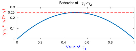
Figure 4.
value with respect to . This value is close to zero when one source is dominant, and has a maximum value of 0.25 when two sources are evenly mixed.
Figure 5 shows with different values assigned. If , grows as increases, and has the maximum at , which is the most difficult case. For , the graph is upside down, so the easiest cases ( and 1) will have the maximum weights. We apply the weight in Equation (15) to the loss function in Equation (4) to obtain a new weighted loss function:
| Algorithm 3 Curriculum Learning |
|
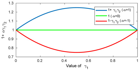
Figure 5.
Loss weight with respect to when (solid line) and (dashed). In the case of , time-frequency bins which two sources are mixed equally has large weights. In the case of , ones which one source is dominant has large weights.
In Equation (15), we can use to choose where to focus during learning. The value of is set differently according to the learning stages to obtain the proposed curriculum learning algorithm. Here, we can choose . Figure 5 shows that when is −1, it focuses on the parts that are easily separable, and when is 1, it focuses on the parts that are hardly separable. In the first stage of training, is set to −1 so that the model should focus on the easily separable parts. The model is expected to quickly learn the overall characteristics of each source early in the training. In the next stage, is set to 0 and the model then learns the whole data evenly. In the last stage, the is set to 1 and the model focuses on time-frequency regions that are difficult to separate. Thus, the model can be learned more sophisticatedly with difficult samples in the later stages of the training phase to improve the final performance of the model. Algorithm 3 summarizes the detailed procedure of the proposed curriculum learning method.
4. Evaluation
We performed singing voice separation experiments and compared the result of the proposed approach with that of baseline approaches. We adopted a stacked RNN [4,5,6] and a U-Net [7,29] as baseline models. Separation experiments were carried out on the simulated vocal-instrument recordings generated by mixing the sound sources from MIR-1K [30], ccMixter [31], and MUSDB18 [32] datasets.
4.1. Separation Model Configuration
The audio file format is mono and 16 kHz PCM (pulse code modulation). To obtain spectrogram features from audio signals, we applied STFT to each analysis frame of 64 milliseconds (1024 samples), while making a 25% overlap with a shift size of 16 milliseconds. After STFT, only the first half of the STFT frequency bins are used because the second half is the complex conjugate of the first one. The number of frequency bins of the STFT spectrogram in Equation (2) is the half of the frame size, . The extracted spectrogram features are component-wisely rescaled so that all the elements belong to .
The first baseline model is implemented by a stacked RNN similar to that in References [4,5,6]. The number of layers and the number of hidden nodes in each layer are set to 3 and 1024, respectively. ReLU activation functions are used for all layers including the output, because spectral magnitudes are nonnegative. Hence, no further post-processing is required. The second baseline is an U-Net implemented by the description given in References [7,29]. Its detailed architecture is given in Table 1. The encoder consists of six convolution layers with a kernel size of 5 and a stride of 2. Each layer uses batch normalization [33] and leakyReLU [34] with 0.2 sloop. The encoder consists of six transposed convolution layers with a kernel size of 5 and a stride of 2. As shown in Table 1, the number of channels of the encoder in each layer doubles in the next layer, except layer 0. At the decoder, the number of channels decreases by half in the next layer to reconstruct the spectrogram as the original size.
Each layer uses a batch normalization and a plain ReLU activation function [34]. The first three layers of the decoder use dropout [35] with the drop probability of 0.5. All models are trained by Adam optimizer [36] with its initial learning rate of and a batch size of 128. The number of training steps of each model is 10,000. Baseline models use the mean squared error (MSE) loss given in Equation (4), and the proposed method uses the weighted loss function in Equation (16) with the weights computed by Equation (15). All the experiments are performed on an Intel i5 4-core desktop computer with 64 gigabytes main memory, equipped with NVIDIA GTX 1080 GPU with 8 gigabytes memory. The batch size (128) was determined considering that the GPU memory should hold all the weights of a single batch to compute the gradients of the weights at the same time.
4.2. Memory and Computational Complexity Analysis
The proposed curriculum learning requires additional computation and memory space. The parameters to be computed are
To calculate in Equation (13), it requires three square operations, an addition, and a division. requires an additional subtraction. If the unit time for basic floating-point operations is identical, the additional number of calculations is 6 for each time-frequency bin, thus making the total amount of operations for T frames and F frequency bins to be . Weight calculation requires two multiplications and an addition, and loss function weighting requires a multiplication, so it totally costs 4 unit times for each time and frequency bin. The total amount of loss function update is . In total, the proposed curriculum learning approach requires of unit computation time for each iteration in training of the networks. These additive computation only updates the final loss function, so it does not depend on the network architecture. The stacked RNN has three hidden layers of 1024 output units, and they should be computed for each sample, . The number of weights in the stacked RNN is roughly defined by input dimension output dimension , so the additional computation is negligible in training. As shown in Table 1, the U-Net also requires large number of weights but additional computation (10 units per input) slightly affects the computation time.
In terms of memory resources, the proposed learning method requires memory spaces to store variables and w in Equations (13) and (15). Total number is , and each variable is stored as 4-byte float data. The number of frames refers to the batch size in batch gradient learning, so in our experiments. F is the number of frequency bins of the spectrogram, which is a half of the STFT analysis size, so . Therefore, the required memory space for a single batch is bytes = kilobytes. We used NVIDIA GTX 1080 GPU with 8 gigabytes memory, so the additional memory space can be disregarded in training models. Because the network architecture is the same, there is no difference in computation and the number of model parameters, and a testing procedure of the proposed model is same as that of the baseline model. Although the training time varies with the model configuration, 10,000 training steps were usually conducted within an hour.
4.3. Experimental Results of MIR-1K Dataset
Singing voice separation experiments with simulated mixtures were performed on the MIR-1K dataset [30] to verify the effectiveness of the proposed methods. This dataset consists of 1000 clips extracted from 110 karaoke recordings sung by 19 Chinese amateur singers. The sound files in this dataset contain instrument and vocal sounds in the left and right channels, respectively. All the stereo sound files are converted to mono and 16 kHz PCM format. We used clips of one male (‘Abjones’) and one female (‘Amy’) singer for training set, and clips of the remaining 17 singers were assigned to the test set. Input mixture signals are generated by simple additions, , for each pair of song clips. Figure 6 represents the distribution of on training set of MIR-1K dataset. is distributed highly around 0 and 1, which are from the regions where only a single source is present.
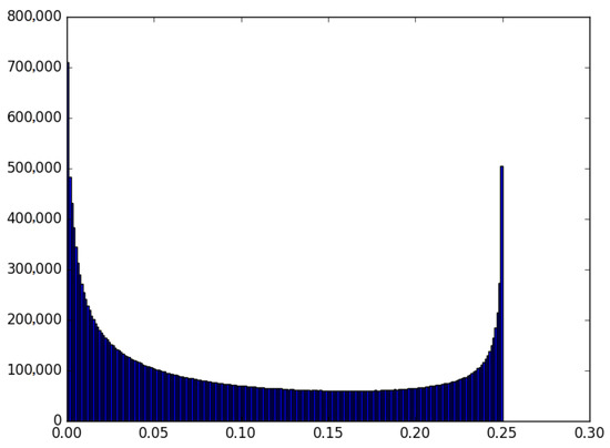
Figure 6.
Distribution of on training set of MIR-1K dataset. is distributed between [0, 0.25].
The performance was evaluated by global normalized source to distortion ratio (GNSDR), global source to interference ratio (GSIR), and global source to artifact ratio (GSAR) values, which are the weighted mean of the NSDRs, SIRs, SARs, respectively, using each frame length as the weight of the corresponding frame [4,26]. Normalized SDR (NSDR) is defined by an increase in SDR after separation. GSIR measures how much uninterested interference is present, GSAR measures how much irrelevant artifact sound exists in the separated results, and GNSDR considers both. The detailed definition of SIR, SDR, and SAR metrics can be found in BSS-EVAL 3.0 [26].
Table 2 shows the results of the experiments performed on the MIR-1K dataset. Subscript m in , , and means that the target source is musical instrument sound, so they measure the performances of instrument sound extraction from the input mixture. In the same way, , , and measure the performances of vocal sound extraction from the mixture. For RNN, the three measures of instrument sound extraction, , , and , were all improved by the proposed curriculum learning. The interfering vocal sound was removed quite well as shown by the increment, from 11.72 dB to 12.30 dB. In the case of vocal sound extraction, was increased by 0.46 dB, but was decreased by 0.44 dB. It means that the proposed method left more music but less unwanted artifact in the separated vocal sound. The overall performance by showed 0.27 dB increment with the proposed. For U-Net, the improvements were similar but mostly vocal extraction was better than music extraction. This might be caused by the property of U-Net using localized convolution windows that provide positive effects to vocal sounds in which gain and frequency characteristics change more often over time than instrument sounds.
Table 2.
Comparison of separation performance for MIR-1K dataset by global normalized source to distortion ratio (GNSDR), global source to artifact ratio (GSAR) and global source to interference ratio (GSIR). “Instrument” columns with subscript “m” are the evaluation results of instrument sound extraction, and “Vocal” columns with subscript “v” are those of vocal sound extraction. The baseline models are stacked RNN (“RNN” row) and U-Net (“U-Net” row). The rows with “proposed” header are the models trained by the proposed curriculum learning method.
4.4. Experimental Results of ccMixter Dataset
The ccMixter dataset [31] consists of 50 songs of various genres, the total length of which is approximately 3 hours. This dataset provides a set of songs consisting of a vocal sound, an instrument sound, and their mixture. Each song is sampled at 41 kHz, so it is downsampled to 16 kHz for the separation experiments. Setups for the spectrogram extraction is the same as that of MIR-1K dataset. We used 10 songs with singer names beginning with A to J for test, and the remaining 40 songs for training the models.
Table 3 shows the results of the experiments performed on the ccMixter dataset [31]. In the music results, the proposed learning improved by 0.27 dB with the RNN, and 0.14 dB with the U-Net. Interestingly, was degraded with the RNN, while it was improved with the U-Net. In the case of , opposite results were observed. One of the reasonable explanations is that, because U-Net focuses more on better reconstruction of the original input, removing interfering sound should be preferred rather than eliminating unwanted artifacts. In the vocal extraction results, most of the values were improved except slight degradation in . The final increments are 0.74 dB with the RNN and 0.41 dB with the U-Net, which is much larger than the values. We used only two singers in the training set of MIR-1K, but there are up to 40 different singers in the training set of ccMixter. So more significant improvements were obtained with vocal extraction results. However, music extraction results were generally worse with ccMixter than with MIR-1K, because of the size of the dataset (50 songs and 110 songs).
Table 3.
Separation performance comparison for ccMixter dataset. Notations are same as in Table 2.
4.5. Experimental Results of MUSDB18 Dataset
MUSDB18 [32] is a much larger dataset than MIR-1K and ccMixter. The training set consists of totally 100 songs, approximately 10 hours long, and the test set consists of 50 songs. This dataset is a multitrack format consisting of five streams that are divided into mixtures, drums, bass, rest of the accompaniment and vocals. The multitrack mixture is used as inputs, and only vocal sounds are extracted from the mixture. The sum of all the other instrument sounds is considered as instrument sounds in the experiments.
Table 4 shows the results of the experiments performed on the MUSDB18 dataset [32]. The most significant increment was observed in in RNN, 1.69 dB, but there were decrement in and of U-Net. The overall performance measured by values were all increased. The smallest and the highest results were 0.38 dB and 1.06 dB. These results show that the proposed method is also effective for large datasets as well.
Table 4.
Separation performance comparison for MUSDB18 dataset. Notations are same as in Table 2.
5. Discussion
In this paper, we propose a method of applying curriculum learning to singing voice separation by adjusting the weight of the loss function. In order to apply curriculum learning, it is necessary to set the difficulty level of each data. We hypothesized that the model is easy to learn characteristics when one source component is dominant. The dominance of each source can be defined by the ratio of one source to the other, which can be obtained from the training data. Using this definition of source dominance, we can apply curriculum learning to singing voice separation by learning more of the different difficulty levels for each train stage. We conducted three experiments to verify the effectiveness of this method. GNSDR was significantly improved by at least 0.12 dB and up to 1.64 dB for two models and three data sets. These experimental results show that the proposed curriculum learning is effective in hard problems such as singing voice separation.
Author Contributions
Conceptualization, S.K. and G.-J.J.; methodology, S.K.; software, S.K.; validation, S.K. and G.-J.J.; formal analysis, S.K., J.-S.P. and G.-J.J; investigation, J.-S.P. and G.-J.J.; resources, S.K.; data curation, S.K.; writing–original draft preparation, S.K.; writing–review and editing, J.-S.P. and G.-J.J.; visualization, S.K.; supervision, J.-S.P. and G.-J.J.; project administration, G.-J.J.; funding acquisition, G.-J.J. All authors have read and agree to the published version of the manuscript.
Funding
This work was supported by Institute for Information and communications Technology Promotion (IITP) grant funded by the Korea government (MSIT) (No. R7124-16-0004, Development of Intelligent Interaction Technology Based on Context Awareness and Human Intention Understanding), the National Research Foundation of Korea (NRF) grant funded by the Korea government (MSIP) (No. NRF-2017M3C1B6071400), and the BK21 Plus project funded by the Ministry of Education, Korea (21A20131600011).
Conflicts of Interest
The authors declare no conflict of interest.
Abbreviations
The following abbreviations are used in this manuscript:
| STFT | Short-Time Fourier transform |
| CNN | Convolutional Neural Network |
| RNN | Recurrent Neural Network |
| CRNN | Convolutional Recurrent Neural Network |
| GAN | Generative Adversarial Network |
| GNSDR | Global Normalized Source to Distortion Ratio |
| GSIR | Global Source to Interference Ratio |
| GSAR | Global Source to Artifact Ratio |
References
- Lin, K.W.E.; Balamurali, B.T.; Koh, E.; Lui, S.; Herremans, D. Singing Voice Separation Using a Deep Convolutional Neural Network Trained by Ideal Binary Mask and Cross Entropy. Neural Comput. Appl. 2020, 32, 1037–1050. [Google Scholar] [CrossRef]
- Takahashi, N.; Mitsufuji, Y. Multi-scale multi-band densenets for audio source separation. In Proceedings of the 2017 IEEE Workshop on Applications of Signal Processing to Audio and Acoustics (WASPAA), New Paltz, NY, USA, 15–18 October 2017; pp. 21–25. [Google Scholar]
- Chandna, P.; Miron, M.; Janer, J.; Gómez, E. Monoaural audio source separation using deep convolutional neural networks. In Proceedings of the International Conference on Latent Variable Analysis and Signal Separation, Grenoble, France, 21–23 February 2017; pp. 258–266. [Google Scholar]
- Huang, P.S.; Kim, M.; Hasegawa-Johnson, M. Joint Optimization of Masks and Deep Recurrent Neural Networks for Monaural Source Separation. IEEE/ACM Trans. Audio Speech Lang. Process. 2015, 23, 2136–2147. [Google Scholar] [CrossRef]
- Huang, P.S.; Kim, M.; Hasegawa-Johnson, M.; Smaragdis, P. Singing-Voice Separation From Monaural Recordings Using Deep Recurrent Neural Networks. In Proceedings of the International Society for Music Information Retrieval Conference (ISMIR), Taipei, Taiwan, 27–31 October 2014; pp. 477–482. [Google Scholar]
- Huang, P.S.; Kim, M.; Hasegawa-Johnson, M.; Smaragdis, P. Deep learning for monaural speech separation. In Proceedings of the IEEE International Conference on Acoustic, Speech and Signal Processing (ICASSP), Florence, Italy, 4–9 May 2014; pp. 1562–1566. [Google Scholar]
- Jansson, A.; Humphrey, E.; Montecchio, N.; Bittner, R.; Kumar, A.; Weyde, T. Singing voice separation with deep U-Net convolutional networks. In Proceedings of the 18th International Society for Music Information Retrieval (ISMIR) Conference, Suzhou, China, 23–27 October2017; pp. 745–751. [Google Scholar]
- Oh, J.; Kim, D.; Yun, S. Spectrogram-channels u-net: A source separation model viewing each channel as the spectrogram of each source. arXiv 2018, arXiv:1810.11520. [Google Scholar]
- Lluís, F.; Pons, J.; Serra, X. End-to-end music source separation: Is it possible in the waveform domain? arXiv 2018, arXiv:1810.12187. [Google Scholar]
- Stoller, D.; Ewert, S.; Dixon, S. Wave-U-Net: A Multi-Scale Neural Network for End-to-End Audio Source Separation. arXiv 2018, arXiv:1806.03185. [Google Scholar]
- Bengio, Y.; Louradour, J.; Collobert, R.; Weston, J. Curriculum Learning. In Proceedings of the International Conference on Machine Learning (ICML), Montreal, QC, Canada, 14–18 June 2009; pp. 41–48. [Google Scholar] [CrossRef]
- Gong, C.; Tao, D.; Maybank, S.J.; Liu, W.; Kang, G.; Yang, J. Multi-Modal Curriculum Learning for Semi-Supervised Image Classification. IEEE Trans. Image Process. 2016, 25, 3249–3260. [Google Scholar] [CrossRef] [PubMed]
- Li, S.; Zhu, X.; Huang, Q.; Xu, H.; Kuo, C.J. Multiple Instance Curriculum Learning for Weakly Supervised Object Detection. arXiv 2017, arXiv:1711.09191. [Google Scholar]
- Wang, J.; Wang, X.; Liu, W. Weakly-and Semi-supervised Faster R-CNN with Curriculum Learning. In Proceedings of the 2018 24th International Conference on Pattern Recognition (ICPR), Beijing, China, 20–24 August 2018; pp. 2416–2421. [Google Scholar]
- Ilg, E.; Mayer, N.; Saikia, T.; Keuper, M.; Dosovitskiy, A.; Brox, T. Flownet 2.0: Evolution of optical flow estimation with deep networks. In Proceedings of the IEEE Conference on Computer Vision and Pattern Recognition, Honolulu, HI, USA, 21–26 July 2017; pp. 2462–2470. [Google Scholar]
- Graves, A.; Bellemare, M.G.; Menick, J.; Munos, R.; Kavukcuoglu, K. Automated curriculum learning for neural networks. In Proceedings of the 34th International Conference on Machine Learning-Volume 70, Sydney, Australia, 6–11 August 2017; pp. 1311–1320. [Google Scholar]
- Takahashi, N.; Goswami, N.; Mitsufuji, Y. MMDenseLSTM: An efficient combination of convolutional and recurrent neural networks for audio source separation. In Proceedings of the 2018 16th International Workshop on Acoustic Signal Enhancement (IWAENC), Tokyo, Japan, 17–20 September 2018; pp. 106–110. [Google Scholar]
- Stöter, F.R.; Uhlich, S.; Liutkus, A.; Mitsufuji, Y. Open-Unmix - A Reference Implementation for Music Source Separation. J. Open Source Softw. 2019. [Google Scholar] [CrossRef]
- Krizhevsky, A.; Sutskever, I.; Hinton, G.E. ImageNet Classification with Deep Convolutional Neural Networks. Adv. Neural Inf. Process. Syst. 2012, 25, 1097–1105. [Google Scholar] [CrossRef]
- Simonyan, K.; Zisserman, A. Very Deep Convolutional Networks for Large-Scale Image Recognition. arXiv 2014, arXiv:1409.1556. [Google Scholar]
- Chan, A.H.S.; Ao, S.I. Advances in Industrial Engineering and Operations Research; Springer: Berlin/Heidelberg, Germany, 2008. [Google Scholar]
- Févotte, C.; Bertin, N.; Durrieu, J.L. Nonnegative Matrix Factorization with the Itakura-Saito Divergence: With Application to Music Analysis. Neural Comput. 2009, 21, 793–830. [Google Scholar] [CrossRef] [PubMed]
- Lefèvre, A.; Bach, F.; Févotte, C. Itakura-Saito nonnegative matrix factorization with group sparsity. In Proceedings of the IEEE International Conference on Acoustic, Speech and Signal Processing (ICASSP), Prague, Czech Republic, 22–27 May 2011; pp. 21–24. [Google Scholar]
- Févotte, C.; Idier, J. Algorithms for Nonnegative Matrix Factorization with the β-Divergence. Neural Comput. 2011, 23, 2421–2456. [Google Scholar] [CrossRef]
- Oja, Z.L.Y. Selecting β-Divergence for Nonnegative Matrix Factorization by Score Matching. In Proceedings of the International Conference on Artificial Neural Networks and Machine Learning (ICANN), Lausanne, Switzerland, 11–14 September 2012; pp. 419–426. [Google Scholar] [CrossRef]
- Vincent, E.; Rémi Gribonval, C.F. Performance measurement in blind audio source separation. IEEE Trans. Audio Speech Lang. Process. 2006, 14, 1462–1469. [Google Scholar] [CrossRef]
- Lotfian, R.; Busso, C. Curriculum learning for speech emotion recognition from crowdsourced labels. IEEE/ACM Trans. Audio Speech Lang. Process. (TASLP) 2019, 27, 815–826. [Google Scholar] [CrossRef]
- Luo, Y.; Chen, Z.; Mesgarani, N. Speaker-independent speech separation with deep attractor network. IEEE/ACM Trans. Audio Speech Lang. Process. 2018, 26, 787–796. [Google Scholar] [CrossRef]
- Ronneberger, O.; Fischer, P.; Brox, T. U-Net: Convolutional Networks for Biomedical Image Segmentation. In International Conference on Medical Image Computing and Computer-Assisted Intervention; Springer: Cham, Germany, 2015. [Google Scholar]
- Hsu, C.L.; Jang, J.S.R. On the Improvement of Singing Voice Separation for Monaural Recordings Using the MIR-1K Dataset. IEEE Trans. Audio Speech Lang. Process. 2010, 18, 310–319. [Google Scholar]
- Liutkus, A.; Fitzgerald, D.; Rafii, Z. Scalable audio separation with light kernel additive modelling. In Proceedings of the IEEE International Conference on Acoustic, Speech and Signal Processing (ICASSP), Brisbane, Australia, 19–24 April 2015. [Google Scholar]
- Rafii, Z.; Liutkus, A.; Stöter, F.R.; Mimilakis, S.I.; Bittner, R. The MUSDB18 corpus for music separation. Zenodo 2017. [Google Scholar] [CrossRef]
- Ioffe, S.; Szegedy, C. Batch Normalization: Accelerating Deep Network Training by Reducing Internal Covariate Shift. In Proceedings of the International Conference on Machine Learning (ICML), Lille, France, 6–11 July 2015; Volume 37, pp. 448–456. [Google Scholar]
- Maas, A.L.; Hannun, A.Y.; Ng, A.Y. Rectifier Nonlinearities Improve Neural Network Acoustic Models. In Proceedings of the International Conference on Machine Learning (ICML), Atlanta, GA, USA, 16–21 June 2013; Volume 30. [Google Scholar]
- Srivastava, N.; Hinton, G.; Krizhevsky, A.; Sutskever, I.; Salakhutdinov, R. Dropout: A Simple Way to Prevent Neural Networks from Overfitting. J. Mach. Learn. Res. 2014, 15, 1929–1958. [Google Scholar]
- Kingma, D.P.; Ba, J. Adam: A Method for Stochastic Optimization. In Proceedings of the International Conference on Learning Representations (ICLR), San Diego, CA, USA, 7–9 May 2015. [Google Scholar]


© 2020 by the authors. Licensee MDPI, Basel, Switzerland. This article is an open access article distributed under the terms and conditions of the Creative Commons Attribution (CC BY) license (http://creativecommons.org/licenses/by/4.0/).