A Novel Optimization Framework to Replicate the Vibro-Acoustics Response of an Aircraft Fuselage

Abstract

In this work, a novel optimization framework, based on a Multi-Disciplinary Optimization (MDO) procedure, applied to the vibro-acoustic Finite Element Method (FEM) model of an aircraft fuselage mock-up, is proposed. The MDO procedure, based on an Efficient Global Optimization (EGO)-like approach, is implemented to characterize acoustic sources that replicate the sound pressure field generated by the engines on the fuselage. A realistic sound pressure field, evaluated by aeroacoustic simulations, was considered as the reference acoustic load, whereas two equivalent sound fields, displayed by two different arrays of microphones and generated by the same configuration of monopoles, were calculated by the proposed vibro-acoustic FEM-MDO procedure. The proposed FEM-MDO framework enables to set up ground experimental tests on aircraft components, useful to replicate their vibro-acoustic performances as if tested in flight. More in general, such a procedure can also be used as a reference tool to design simplified tests starting from more complex ones.

1. Introduction

Nowadays, an accurate evaluation of noise generation and propagation has become a key concern, especially in the areas in which the comfort for end users has become a turning point. An increasing interest of aerospace and automotive industries for the passengers’ comfort has been providing the framework in which these issues have acquired a prominent role. The typical topics to be tackled for investigations of noise and vibrations of vehicles, aircraft, space launchers, etc. deal with aerodynamically generated noise, engine noise, Passive Noise Control (PNC), Active Noise Control (ANC) and assessment of acoustic properties of innovative materials [1]. The reduction of acoustic emissions and the improvement of interior comfort are on the path of all major industries of the transport system, having a direct impact on customer satisfaction and, consequently, on the commercial success of new products.

Nowadays, the aeronautics industry requires several experimental tests during the designing processes that, very often, present huge costs and generally are not simple to carry out with a reasonable accuracy.

In this work, a Finite Element Method-Multi-Disciplinary Optimization (FEM-MDO) framework has been proposed to characterize sets of acoustic sources that replicate the sound field produced by the real engines on an aircraft fuselage mock-up. This procedure would enable to set up ground experimental tests on aircraft components, useful to replicate their vibro-acoustic performances as if tested in flight. More in general, it can also be used as a reference tool to design simplified tests for complex problems.

Similar approaches in which simplified acoustic sources were used to simulate more complex acoustic fields can be found in literature, e.g., the noise generated by rocket engines in [2,3,4,5]. In fact, in these works a semi-empirical jet noise model has been exploited and adapted for reconstructing the experimental acoustic near field on the external surface of a space launcher, allowing an affordable vibro-acoustic assessment based on the achieved pressure excitation. The reference theory to predict the noise radiated by rotors can be found in [6,7], in which Lighthill originally developed the first aeroacoustics analogy that, in the last decades, has been extensively applied in numerical aeroacoustics to reduce the complex sound sources to simple emitter types. In general, aeroacoustic analogies were derived from the compressible Navier–Stokes equations, rearranged into forms of the inhomogeneous acoustic wave equation. Some approximations were introduced to make the source terms independent of the acoustic variables and, in this way, linearized equations were derived to describe the propagation of the acoustic waves in a homogeneous resting medium.

The original formulation of Lighthill was extended by Ffowcs Williams [8] to take into account vibrating solid surfaces, by rearranging the Navier–Stokes equations with introduction of source terms composed by:

• quadrupole sources, generated by the turbulence of the fluid;
• dipole sources, caused by fluctuations of the fluid-structural interaction forces;
• monopole sources, generated by mass fluctuations.

These theories do not provide any indication about the positioning of sources that commonly are characterized by means of Computational Fluid Dynamics (CFD) simulations and located in correspondence of the geometrical central axis of the engine rotors. These theories are also still inefficient under near field conditions. Thus, it is commonly necessary to proceed numerically to determine type, number and position of the acoustic sources in the most complicated cases. Such numerical procedures allow to approximately replicate the real acoustic pressure fields generated by the engines via ordinary acoustic sources. In this way, the experimental testing could be carried out either in anechoic or semi anechoic environments with the emulated acoustic field imposed by loudspeakers.

If successful, this procedure would provide a preliminary step to go further in the prediction of cabin noise: the next step could be the monitoring of cabin noise as produced by the engine rotors, by adding microphones in a realistic mock-up placed in an equipped laboratory.

2. Problem Description

This work can be split in three main parts.

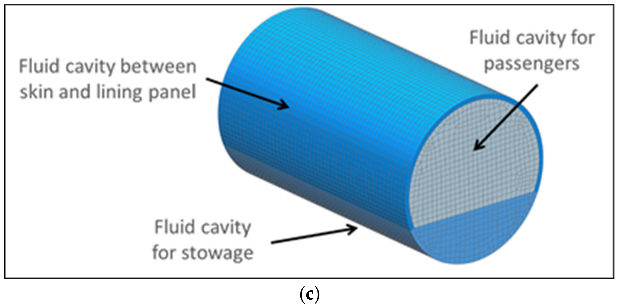
The first part comprises the CAD/FEM modeling of an aircraft fuselage mock-up in order to build up a simplified vibro-acoustic FEM model. Such a model was used to perform the vibro-acoustic analyses of the fuselage when loaded either with the sound pressure emitted by the engines, or with the sound pressure emulated by different sets of simple acoustic sources (monopoles).

The second part comprises the set-up of the MDO procedure, with the aim of characterizing the previously given sets of acoustic sources in order to reproduce, in a simplified manner, the reference pressure field. Moreover, such a procedure was performed two times in order to calculate, for a given configuration of acoustic sources, the results of two different configurations of microphones (two separate sets of simulations were run).

The last part comprises the presentation of results for the two simulated cases and their comparisons with the reference data. A discussion on such results is also provided and recommendations for further improvements are added.

3. CAD/FEM Modeling

3.1. FEM Mesh

The FEM model was built up by the commercial code Siemens NX Nastran 12.0 [9].

Starting from a CAD model of a fuselage barrel (Figure 1), an FEM model was generated comprising 2D/1D structural parts and 3D internal and external fluid volumes.

The 2D structural part represented the key contributor to the vibration response of the model, and comprised four main surfaces made out of different materials (Figure 2a):

• the external surface on which the external acoustic pressure directly impacts;
• the lining panel, realized by a sandwich suitable to reduce noise and vibration, to improve the comfort inside the cabin;
• the floor on which seats are located (seats were not modeled in this work);
• the window glasses.

The 1D structural elements (Figure 2b) were divided in: longerons and circumferential beams to stiffen the structure, transversal and axial floor support, formed by beams with different sections, windows frameworks and doors. Furthermore, the sandwich was linked to axial and circumferential beams by elastic and rigid constraints.

The internal fluid cavities (Figure 2c) were: the cabin occupied by passengers, the stowage under the floor, the volume displaced between the external surface and the internal lining panels.

The external air was modeled to let the sound waves propagate from the monopole sources, representative of the MDO inputs, to the structure. The external fluid modeling was also essential to measure the Acoustic Intensities (AIs), representative of the MDO outputs, in the 30 microphone locations on the external fuselage surface. Such external fluid was modeled as a cube of solid elements with a cavity in the center to accommodate the fuselage barrel. Such cube was modeled with a size large enough to comprise at least 2 wavelengths at the frequency of interest. This was required in order to prevent boundary effects since the condition of non-reflecting boundary condition was applied at the boundaries to simulate the infinite radiation [9]. The mesh comprised tetrahedral solid linear elements with variable size having at least 6 nodes per wavelength, in order to have an acceptable accuracy for fluid field calculation in the fluid-structure interface zone (close to the structure); larger elements were adopted far from the structure in order to reduce the computational burden (Figure 3b). Even if the accuracy could turn out to be not so high with 6 nodes per wavelength, it is not a problem for this work where the aim is to show that the proposed procedure is a viable approach for reducing the experimental effort, based on an acceptable agreement between the reproduced and the reference sound pressure distribution on the fuselage. More info about the level of approximation inherent the mesh density adopted could be retrieved in [10,11].

In [10], two numerical examples, a long duct and a sedan cabin compartment have been analyzed. In the first example, the analytical solution of the corresponding one-dimensional boundary value problem has been used for comparison. Numerical investigations limited to the frequency range of 0 < kl < 80 *Pi essentially confirmed the common rules of modeling that six constant or bilinear elements per wavelength are sufficient to obtain a solution of about 10 to 15% error. The common rule of six linear elements per wavelength, provide an error inferior than 10% in the Euclidean norm and inferior than 20% in the maximum norm. The second example confirmed most of these conclusions.

In [11], Zaleski investigated discretization requirements for sound radiation at complicated structures. He confirmed the rule of six linear boundary elements per wavelength to achieve an acceptable accuracy in the sound pressure for lower wave numbers, whereas the rule of a fixed number of elements per wavelength may be invalid for high wave numbers.

3.2. Reference Case (RC) and Simplified Cases (SC)

The so obtained vibro-acoustic FEM model was preliminary solved by considering as acoustic load the pressure on the external skin calculated by aeroacoustic calculations (Figure 4). This simulation was termed as Reference Case (RC) because it provided the benchmark to assess the Simplified Cases (SCs). Such pressure distribution outside the fuselage was obtained by aeroacoustic simulations, based on the integral formulation of Ffowcs Williams and Hawkings [8], and considered the rotating engine rotors, at the first Blade Passage Frequency (1BPF), as the only noise contributor providing periodic low frequency loads on the structure. It was considered just the 1BPF because it was the most relevant under cruise flight condition.

From Figure 4, it can be qualitatively noticed that the acoustic pressure load shape was caused by the phase shift of the engine rotors (an arbitrary non-null value was selected in this case), and the increment of the load amplitude in the axial direction, as a consequence of the distance reduction from the rotors position. The circumferential distribution of pressure loads presents a complex pattern, clearly variable as a function of the imposed phase shift.

More in general, given the model being available, the calculation of additional frequencies or noise contributors does not impose additional complications apart from the calculation time.

Subsequently, the boundary condition corresponding to the pressure distribution was removed from the FEM model and a set of acoustic sources and microphones (monitoring points) was added. Such modified FEM model, after a vibro-acoustic coupled analysis, provided the results to be used as input for the MDO procedure.

In particular, a given set of acoustic sources and two different sets of microphones were considered, termed in the followings as SCs: SC1 and SC2. The two SCs correspond to two attempts to replicate the RC, namely, to replicate the realistic reference solution in terms of acoustic pressure outside the fuselage and, consequentially, in terms of vibro-acoustic response of the structure.

Figure 5 shows the number (four) and positions of the acoustic monopole sources designed to try reproducing the reference sound field and providing the input for the MDO iterations.

Figure 6 highlights number and position of the microphones required to measure the Acoustic Intensities (AIs) outside the fuselage. Such microphones were required in order to monitor the pressure field on the fuselage surface for each MDO iteration. Two kinds of positioning were considered comprising either 3 or 5 rings having 6 microphones each, for a total of either 18 or 30 microphones.

Such monopoles and microphones were adopted to create two SCs (Figure 6 and Figure 7), i.e.,

• SC1 (Figure 7a), comprising 18 output microphones,
• SC2 (Figure 7b), comprising 30 output microphones.

Both SCs comprised 4 monopole sources positioned as shown in Figure 5.

3.3. Boundary Conditions

Apart from the previously described boundary conditions, all the remaining settings were corresponding for both RC and SCs. In particular, a fully clamped condition (Figure 8a) was imposed at the two ends of the barrel (no translations neither rotations were allowed for such nodes). The two fuselage ending surfaces were considered as acoustically fully reflecting, thus assuming that no interaction between internal and external fluids was allowed. Moreover, the six faces of the cube volume, representative of the external fluid, were modeled as anechoic walls, thus assuming that no reflection was allowed (Acoustically Matched Layer; Figure 8b) [9]. Finally, a strong coupling condition between fluids and structural nodes was set up to allow for a bidirectional interaction between structure and surrounding fluid [9].

Initial sound power amplitudes and phases were assigned for each monopole source and, step-by-step, adjusted by the optimization procedure.

At this stage, the goal of the work was not an accurate reproduction of the real fuselage response to the sound pressure coming from the engines, but only the implementation and validation by comparison between RC and SCs of a general MDO procedure to solve a complex optimization problem such as the one here proposed. It is worth noting that the MDO procedure here proposed required many FEM solutions of the current model to provide a stable solution; therefore, some simplifications were considered as a trade-off between a sufficiently accurate physical replication of the vibro-acoustic fuselage behavior and an acceptable computational burden.

A comparison between the cross sections of the so created FEM models built up for RC and SC is shown in Figure 9.

4. Optimization Process

4.1. Process Integration and Design Optimization (PIDO)

The optimization procedure was implemented in the commercial Process Integration and Design Optimization (PIDO) platform Optimus [12,13]. The software provides a wrapper where different simulation tools (Commercial Off-The-Shelf or specifically created) can be implemented, connected and investigated, using a suite of design and optimization methods. To achieve this automatic analysis of the model behavior, the simulation requires an a priori study to determine its parameters (input variables not under user control), design variables (number, type, range), outputs, constraints (limitations to the design space) and objective(s).

Depending on the structure of the problem and its behavior, different analysis methodologies can be implemented. The first step typically involves one or more Design of Experiments (DOE) to gain knowledge on the design variable to outputs relationship.

A set of experiments, decided using only the range of the design variables (as for the factorial-class methods, or Latin Hypercube methodology just to name some of the most commonly used) is performed and the values of the outputs are studied either directly or involving more elaborate data post-processing as correlation studies, clustering, meta-modeling.

The acquired insight on the problem responses can then be re-used to determine the best algorithm to assess the design that better respond to a specific need (single objective optimization) or satisfies multiple criteria at the same time (multi-objective optimization).

The same general approach can be extended to include uncertainties, both in the variables and the analyses, and perform uncertainties propagation and robust optimization.

4.2. Modeled Problem

In the modeled problem, the sound power and phase of each monopole source represented the input data for the MDO process, whereas the Acoustic Intensities (AIs) at microphones provided the output. Thus, a parametrization of the model for the SCs was required to change the input values for the FEM simulations and to get the output to compare with RC data. Such parametrization of the model was implemented in the PIDO platform, using the related interfaces after an appropriate setup and validation of the FEM model.

The interfaces are designed to simplify the access to the identified model parameters and, during the execution of the analyses, automatically map the desired values of the design variables to the model itself and extract the values of the outputs of interest. The information gathered through analyses are processed to determine the relationships between inputs and outputs; this knowledge can then be passed to different post-process tools or used to perform design optimization, reliability study, robust design.

The same validated workflow with parametrized FEM model, analysis, results extraction and post-process has been used both to perform DOE and optimizations. DOEs have been run both to provide a clear overview of the design variables’ impact and to generate a re-usable database of simulations. Due to the nature of the design variables (and specifically the periodicity of the phase) some of the DOE approaches would have been ineffective (in particular, the members of the factorial-class, that explore the combinations of the lower and higher values of the design variables, but also other methods like the Plackett–Burman are affected by the same limitations). The final objective was to determine configuration of the sources able to provide the best approximation of the known RC pressure field; this has been organized as an optimization problem where a dedicated performance indicator (Equation (1)), able to describe the difference between the reference and the simulated values, had to be minimized. A single averaged, performance indicator was selected.

The problem to be solved was far from trivial; exploratory DOE and subsequent correlation studies highlighted that, although the amplitude of the sources had a relevant and, within certain conditions, predictable impact on the pressure field, the phase was significantly less manageable. PIDO platforms typically rely on black-box optimizers, algorithms that neither have insight on the problem physics, nor make assumptions about its continuity or smoothness.

The initial studies underlined the non-linear and non-monotone behavior of the outputs with respect to design variables; from the optimization point of view, this creates several local minima that hinder the convergence of the algorithm.

Global optimizers are methodologies that explore the whole design space, therefore they are suitable for this kind of problem; however, this exploration requires a relevant number of experiments [14]. On the other hand, local optimizers explore limited regions of the domain and often rely on the analytical or numerical evaluation of the gradient to determine the local solution. They are usually attracted by minima close to the starting point, whose setup becomes critical, although gradient-based line search can be exploited to extend the investigated portion of the domain.

4.3. Efficient Global Optimization (EGO)

Instead of a standard algorithm, a tailored one was created and exploited for this problem; the optimization strategy was an Efficient Global Optimization (EGO) [15] derived methodology, simplified (without the stochastic process model) and customized to better drive the optimization algorithm to find a solution in such a complex optimization problem.

Due to the computational cost of the simulations, the methodology had to be able to re-use all the previous analyses; additionally, surrogate models had been used to approximate the model and identify candidate points without the need for extensive simulation campaigns.

The implemented MDO optimization procedure is composed of an initial DOE (either performed as part of the optimization or previously run) and a sequence of iterations with a stopping criterion. Among the possible DOEs, the Latin Hypercube Design (LHD) [13] was the first choice in force of its extensive design space exploration and orthogonality of the experiments, however, other methods or combination of methods can be used. Traditional DOEs are not iterative in nature, therefore all the experiments are decided before the first analysis is performed. This can limit the effectiveness in identifying the problem characteristics.

For each configuration of the sources, a single, systematic LHD has been performed, accompanied by prior secondary DOEs, mainly used to validate the integration and analysis procedure, and therefore verify their reliability for a wide range of scenarios.

The decision to aim for a single DOE has been driven by the computational effort of the simulations; in order to provide a quantitative representation of the problem (required by its planned applications, namely the database and the metamodels generation, and the non-linear behavior of the outputs), the DOE required a significant number of experiments. In force of the LHD nature, it would have not been possible to perform smaller, independent and differently initialized DOEs and later combine them in a single database while preserving the experiments decoupling. Random initialization has been used.

The main DOE has been merged with the lesser ones (different by both seed and number of experiments) and compared with the unmerged one in terms of correlation (Spearman and Pearson), showing no significant variations.

The general pattern of almost null linear and monotone correlation between phase and outputs and average (around 0.5) between amplitude and outputs has been observed in all the source configurations.

The dataset generated by the optimization procedure can be used to replace (or integrate) the original DOE, due to its compatibility in terms of inputs and outputs.

4.4. MDO Optimization Procedure

The MDO optimization procedure proceeded by iterating the following steps:

• generation of the interpolated response surfaces, based on the DOE table data;
• identification of the best model using cross-validation;
• run of the global optimization method on the response surface, to find a candidate point that minimizes the metrics (Equation (1));
• check of the proximity of the candidate point to the existing samples and, if needed, apply a random shift;
• space-filling, to balance for the global optimization (based on surrogate models with known data) to fall into local minima without performing additional exploration;
• run the FEM analyses on the two new points;
• update the initial DOE data and iterate until a terminate criterion is satisfied.

Thus, the starting point of the MDO strategy is an existing DOE database, not necessarily tailored for optimization. Then, the global optimization method Differential Evolution (DEVOL) [14], was executed to find a “good” candidate point [12] on the Response Surface Method (RSM).

From the algorithm perspective, there are no differences between a run on real analyses or on surrogated models, and this represents a trade-off between accuracy and simulation time. Models reproduce all the outputs of the simulation, including the constraints, in order to preserve results consistency.

The used metamodel, interpolated Radial Basis Functions (RBFs), use multi-quadratic, linear, cubic and thin-plate kernels; other numerical formulations, like approximated or neural-network-based, have been considered but not included.

Every time models are created or updated, their predictive capabilities were evaluated by means of cross-validation, using the R2press regression parameter (PRESS stands for Predicted Residual Error Sum of Squares). Every model is repetitively generated for datasets with one experiment removed and then evaluated on the missing experiment, to compare predicted and simulated results. The results of all these calculations are added into one regression value that, if close to 1, indicates that the model will perform well for points that were not simulated. Only the best model with the highest R2press was used for optimization. The automated validation and selection of the model with the higher predictive capability is part of the functionalities provided by the PIDO platform; the best kernel varied through the campaign but on average, cubic was the most exploited.

Initial value of the cross-validation (DOE only) was low, 0.3 or less in a range between −1 and +1, where +1 indicates that the model’s predictions always match perfectly the reference (the model is iteratively re-built without a sample and the prediction is compared with the sample) whereas post-optimization values were between 0.65 and 0.7. This value is still not enough to provide results without proper validation; all the candidate configurations are investigated numerically and not just on the metamodel.

RBFs have been preferred over approximated ones (such as the least square) for the higher accuracy without significant overhead in their construction (in the order of a few seconds with 300 experiments, 8 inputs, 30 outputs), whereas like Kriging and Light Weight Neural Network had similar accuracy with slightly superior construction time.

Models assembly time was important as this operation was performed for each iteration.

4.5. Global Optimization Method

DEVOL was selected as the global optimization method to guarantee complete coverage of the design space even if its computational burden can represent a drawback. This was not the case for our problem as the evaluation of hundreds of candidate points on the surrogate models was executed in sub-second time. Other algorithms were tested (like Simulated Annealing) achieving comparable results; the accuracy of the RSM was significantly more relevant than the algorithm itself.

Subsequently, a proximity check was performed to avoid oversampling of the same design region and/or “cornered” RSMs, (measuring the distance between the proposed optimal point and the existing experiments). Differences in design variables ranges were removed through a normalization of the design space. The distance was determined using the design variable only, not the results of the simulation.

Candidate points within an arbitrary threshold were moved by a limited, random offset to preserve the general location but avoid duplicated samples, as would happen when the solver is trapped in a local minimum.

The random offset reduces but does not solve entirely, the potential oversampling problem, thus resulting in new experiments still focused on a specific region of the domain.

To address this limitation, a dedicated space-filling was performed; this improved the overall RSM and reduced the chances of local minima traps [16] by setting up one experiment in the less explored region of the design space.

The resulting continuous MaxMin optimization problem was replaced with a discretized version, based on a dense, support LHD [17]. The identification of the design point that has the maximum, minimum distance from all the existing ones requires the evaluation of the distance of all the points in the support from all the previous experiments. L1 norm was used both to reduce the effort and due to its representativeness in higher dimensions [18].

MaxMin and discrete space-filling offer comparable solutions (provided a dense enough support) for single-point applications, whereas if multiple experiments had to be added, the discrete space-filling results were sub-optimal. This limitation has been considered acceptable due to the nature of the envisioned optimization method.

As a final step, the FEM simulations for both candidate and space-filling points were performed, and the results included in the DOE dataset used in the following iterations. From the operative point of view, running two experiments in a single batch was more efficient than 2 separated experiments. The adopted termination criterion was the total number of analyses, whereas the implementation of a convergence check was postponed to a later stage.

The simulation workflow illustrated in Figure 10 was constructed in Optimus to run the MDO process.

This optimization strategy made the structure flexible since the DOE results were independent of the chosen function for the metrics, i.e., the target function; the latter was defined in a python script loaded in the software when calculating the metrics (see Figure 10). The separation between the outputs generated by the simulations and the post processing allowed for different metrics to be tested preserving the experiments database.

The choice of the metric function was a key point of the work in order to get the most appropriate comparison between RC and SC data. Different functions were tested and the current choice (this aspect is still under study) is reported in Equation (1): it represents a normalized percentage difference among the AI values for each microphone:

$$\mathrm{Normalized} \mathrm{metric}=\frac{{{\displaystyle \sum }}_{\mathrm{i}=1}^{\mathrm{n}}\left|\frac{{\mathrm{AI}}_{\mathrm{i}}^{\mathrm{RC}}-{\mathrm{AI}}_{\mathrm{i}}^{\mathrm{SC}}}{{\mathrm{AI}}_{\mathrm{i}}^{\mathrm{RC}}}\right|}{\mathrm{n}}=\frac{\mathrm{metric}}{\mathrm{n}}$$

(1)

where n is the number of microphones, AIRC is the acoustic intensity array for the RC, and AISC is the acoustic intensity array calculated for each iteration. The metric is not entirely symmetric due to the normalization and the fact that AIs are positive only values; the normalization was required due to the reference values range that could be significantly different among the microphones.

5. Results

The MDO procedure iterated changing repeatedly the sound powers and phases of the monopole sources in such a way to get AIs at the microphones for the SCs as close as possible to the AIs calculated for the RC. The results for each SC are reported in the followings.

5.1. SC1 Results

SC1 optimization process was stopped after a predefined (500) number of iterations. The finally obtained AIs are shown in Figure 11 together with the RC data. Figure 12 shows the SC1 whole pressure field on the external skin of the fuselage, where the horizontal axis is the fuselage axis whereas the vertical axis is the angular coordinate around the fuselage.

5.2. SC2 Results

SC2 optimization process elapsed nearly 320 iterations. The final comparison of the so obtained AIs at the microphone locations is shown in Figure 13 together with the RC ones. The whole pressure field on the external skin of the fuselage is reported in Figure 14.

6. Discussion

Figure 11 and Figure 13 show the comparisons between the SCs AIs at the microphones and the AIs for the RC. The reference pressure field in the volume surrounding the barrel is shown in Figure 15. The best metric values (Equation (1)) and the RSM quality R2press index are reported in

Table 1. Best metric values and R²_press for both SCs.

	Best Metric Value [-]	R2press [–]
SC1	0.039	0.951
SC2	0.047	0.983

.

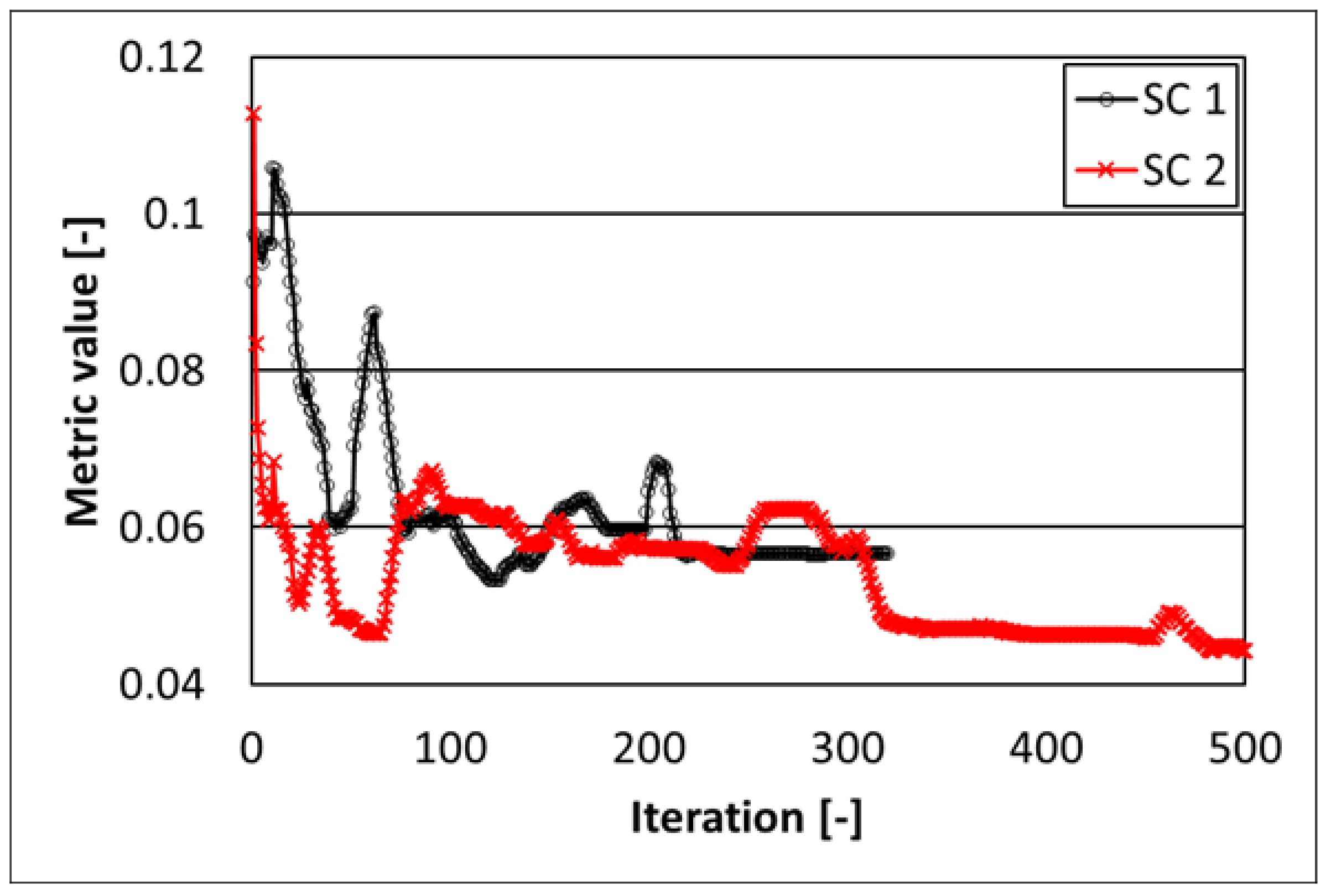
The final metrics values are equal to nearly 4%–5%, stating that the average error between the reference and the simulated data was equal to nearly 4%–5% for each microphone. Such discrepancies were judged as acceptable, especially if considering the complexity of the study case here proposed for the presented optimization algorithm.

The evolutions of the metric values for the two considered SCs vs. iterations are reported in Figure 16. Scattering of data was given by the space filling algorithm, since a “far” candidate point was evaluated for each iteration, thus generally giving a higher metric value. However, the general trend happens to be decreasing for both SCs. This can be confirmed also in terms of R2press index (Table 1).

As a final outcome, the SC2 was judged as more adequate than SC1 to replicate the reference pressure field. This was attributed to the fact that as an overall the pressure field was better captured by the optimization procedure, see Figure 12, Figure 14 and Figure 15 for a qualitative comparison and Table 1 (correlation in terms of R2press index). Thus, the solution with an increased number of microphones rings (3 for SC1 to 5 for SC2) should be selected to better drive the optimization toward a more accurate sound field replication.

7. Conclusions

A novel optimization framework, based on a MDO procedure applied to the vibro-acoustic FEM model of a fuselage mock-up, has been presented in this work.

The MDO procedure, based on an EGO-like approach, has been adopted to characterize acoustic sources that replicate the sound pressure field generated by the engines on the fuselage. A predetermined sound pressure field was considered as a reference data, whereas two tentative sound fields were calculated by leveraging on the proposed FEM-MDO framework.

The comparisons between the reference and the calculated data in terms of pressure fields, quality indexes and metric values, have been judged as acceptable even if further refinements, considering different setup of monopole sources and microphone locations together with a different metrics, are currently under development.

The proposed FEM-MDO procedure can be considered as a potential tool to set up ground experimental tests on aircraft components to replicate their vibro-acoustic performances as if tested in flight.