Stepwise Intelligent Diagnosis Method for Rotor System with Sliding Bearing Based on Statistical Filter and Stacked Auto-Encoder

Abstract

Since the raw signal collected from the sliding bearing is contaminated with background noise, and it is difficult to obtain high-precision results for the traditional methods due to the low signal-to-noise ratio (SNR). Therefore, a stepwise intelligent diagnosis method based on statistical filter and stacked auto-encoder (SAE) that is established with several auto-encoders is proposed to identify several faults of sliding bearing in a rotor system. Firstly, the statistical filter is utilized to reduce the interference information for the different abnormal states and to increase the SNR. Secondly, the stepwise intelligent diagnosis based on SAE is performed to learn the useful fault features, and it can automatically complete the fault diagnosis which is contributed with the superiority binary classification to fully mine the relationship between the fault characteristics and the health condition of bearing. Finally, the diagnosis of the oil whirl and structural faults in a rotor system is cited as an example to demonstrate the effectiveness of proposed method. It can effectively illustrate the advantages of the stepwise diagnosis method to obtain the maximum diagnostic accuracy.

1. Introduction

Sliding bearing is widely used in chemical, metallurgical, steel, and aerospace industries because of its smooth operation, high speed and impact property [1]. However, it is prone to damage due to harsh working environment, which can cause great catastrophes. Therefore, accurate fault diagnosis techniques are necessary to ensure the stable operation of equipment and avoid major safety accidents.

It mainly includes theoretical research and condition monitoring for the sliding bearing fault diagnosis. The former is a classical means to perform the sliding bearing fault diagnosis, such as the mass-conserving boundary condition [2] which can effectively overcome the drawbacks of Reynolds equation [3] to perform fault diagnosis for sliding bearing. However, the problem of film cavitation in this technology is mainly hindrance in numerical calculation based on mass conservation of boundary conditions, which cannot meet requirements of modern industry. Therefore, condition monitoring is a useful and feasible method to perform bearing fault diagnosis [4].

The condition monitoring is mainly divided into vibration signal analysis, oil analysis, and acoustic emission signal analysis. Although oil analysis and acoustic emission signal analysis have unique advantages for strong background noise and early bearing failures, their application are limited due to expensive price. Therefore, vibration signal analysis plays an important role in bearing fault diagnosis, which is mainly divided into two parts, including time domain analysis [5,6] and frequency domain analysis [7]. However, the time domain analysis can only roughly reflect whether the mechanical equipment is normal or not and cannot provide detailed information (fault type, fault location, and fault severity) about the bearing. It can generally be utilized to make simple diagnosis for the equipment. Thus, many studies contribute to utilizing frequency domain technology to identify spectrum structure. Especially in precise diagnosis, the sensitive fault information can be extracted to distinguish the anomaly type [8].

Although the fault feature can well represent the state of the sliding bearing based on above methods, it largely depends on the rich experiments and professional knowledge. It is not only inefficient, but also the accuracy is difficult to guarantee when the worker observes a large amount of data for a long time. Therefore, automatic identification has an extremely important significance for improving the efficiency and reliability of rotating machinery. Furthermore, the traditional methods have drawbacks that can lead to the reduction and loss of signal detail information, which cannot precisely distinguish several faults more efficiently according to the features of various faults [9]. Meanwhile, prior knowledge is more important for those methods and need to be known beforehand. However, it is difficult to get theses precious information for the practical sliding bearing, such as the unbalance, oil whirl, and oil whip in a mechanical system [10].

Therefore, machine learning [11]—such as support vector machine (SVM) [12], back propagation neural network (BPNN) [13], and decision tree [14] has an extremely important significance for improving the efficiency and reliability of the fault diagnosis for sliding bearing. An adaptive neuro-fuzzy inference system [15], which combined multi-scale entropy and adaptive neuro-fuzzy inference system, cannot only reliably discriminate among different fault categories and identify the level of fault severity, but overcome the limitations of traditional data-based models/techniques. Although the reported research has achieved high-precision intelligent diagnosis, it still needs strict requirements for complicated signal processing methods to extract accurate fault characteristics. Moreover, the raw signal is contaminated by intensive background noise that is deceptive to machine learning, reducing accuracy [16]. Furthermore, traditional machine learning will not be able to handle massive data to a certain extent, which will reduce the efficiency of diagnosis due to development of signal acquisition technology.

Deep learning—including convolutional neural network (CNN) [17], deep neural network (DNN), [18] and SAE [19]—can effectively overcome deficiencies above in current intelligent diagnosis methods. It refers to multiple processing layers and simple structures to explore the hidden information of signal for the sliding bearing fault diagnosis. An improved SAE [20] is proposed to overcome fluctuations of the shaft speed, and it outperforms conventional fault diagnosis algorithms in terms of fault classification accuracy. It benefits from data mining ability of SAE to outperform traditional machine learning. However, it is also affected by intensive background noises that can make difficulties for learning the sensitive information to interference diagnostic accuracy. Therefore, the statistical filter performs the purification for the raw signal by removing the noise and giving prominence to the fault feature. Moreover, the fault of the sliding bearing—such as oil whirl, dynamic unbalance, static unbalance, and contact rubbing—are centralized in low frequency or mid-low frequency, with no obvious boundaries between unbalance faults. Therefore, stepwise intelligent diagnosis method based on SAE is proposed to solve problems above to improve the sliding bearing fault diagnosis. It also can overcome the disadvantage that fault feature health status cannot be extracted accurately with the theoretical methods in practice equipment diagnosis process. To sum up, the proposed method has the following novel benefits and solves corresponding problems.

• The proposed method can automatically learn useful fault information with the deep structure of SAE, which cannot depend on rich experiments and professional knowledge to implement intelligent fault diagnosis. Moreover, the statistical filter in the proposed method can attenuate noise effects to extract the sensitive feature further, and it can sensitively reflect the symptoms of the equipment states.
• The proposed method effectively distinguishes five kinds of conditions through the stepwise intelligent diagnosis with the SAE after filtering. Although the various faults similarities in sliding bearing are higher than others in rotor system, it can accurately and efficiently distinguish them in a large number of signals.
• The detail relationship between fault feature and fault type in sliding bearing can be described with the data mining capabilities owning to SAE, which is not affected by the negative impact of the data dimension. Therefore, it can objectively and effectively improve the diagnosis accuracy and enhances the robustness of the proposed method.

To indicate the feasibility and effectiveness of the proposed method, the paper presents detailed experiments for diagnose faults of sliding bearing including contact rubbing, oil whirl, dynamic unbalance, and static unbalance. The experimental results demonstrate that the proposed method can get high-precision fault diagnosis compared with other several methods.

2. Basic Theory

The general procedure of proposed method for sliding bearing fault diagnosis mainly consists of two parts. Firstly, the statistical filter is employed to filter the noise and to extract useful information by conserving difference information comparing with the normal signal through the statistical theory. Then the stepwise intelligent diagnosis method based on SAE is proposed to overcome the difficulties that the fault feature of the sliding bearing has no obvious distinction.

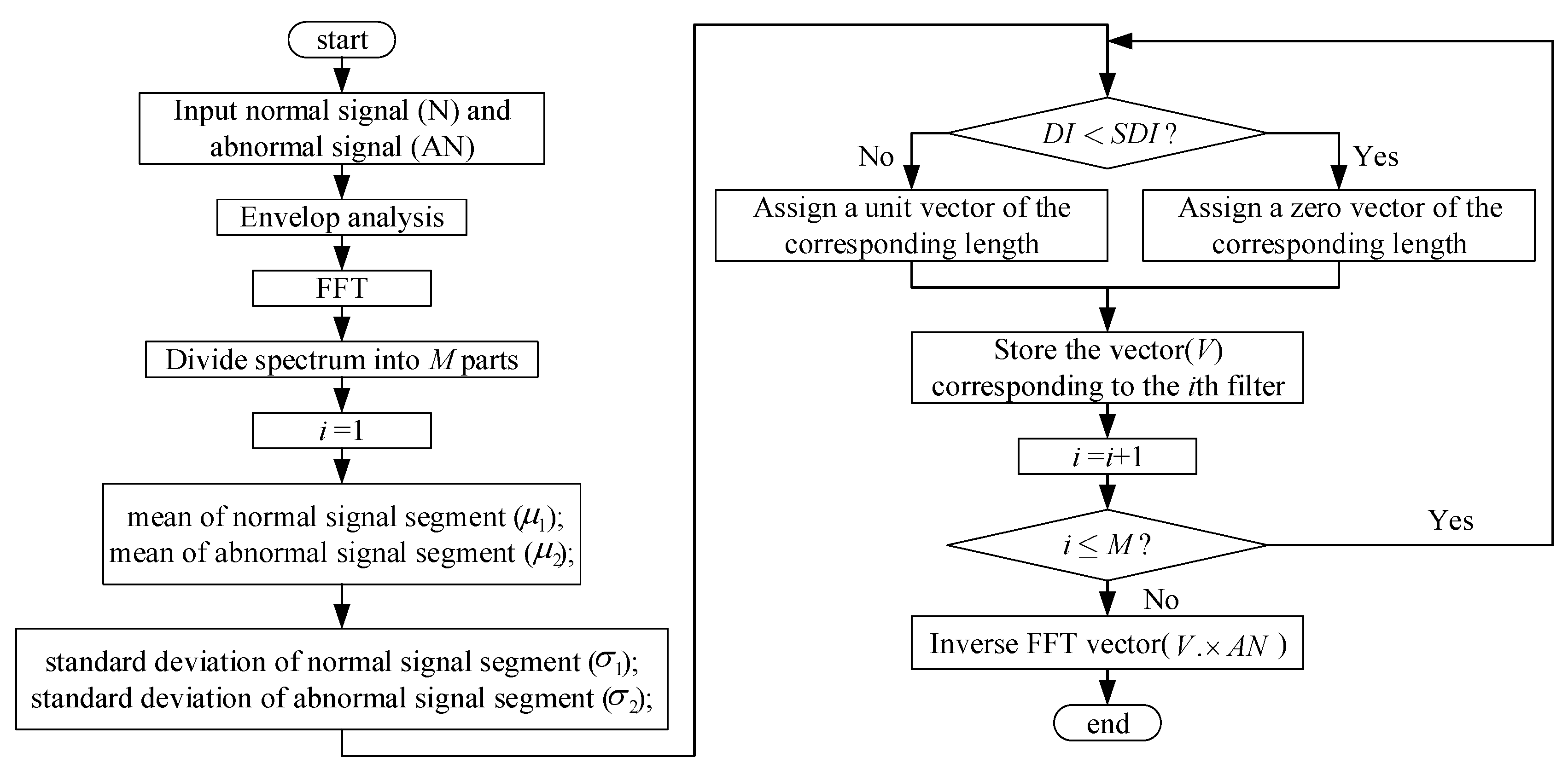
2.1. Basic Concept of the Statistical Filter

Although fault diagnosis of sliding bearings is often artificially carried out with frequency analysis of signals, there is a need for a reliable, automated diagnosis method thereof [21]. However, the effect of the background noise in the signal is serious, and the symptom of five kinds of faults is not evident. Therefore, the purpose of statistical filter is removing the negative effect from the noise and extracts the sensitive information by the statistical method, which can save the abnormal information by comparing the general statistical indicator between the normal signal and abnormal signal, as shown in Figure 1.

The statistical filter removes noise with calculating the mean and standard deviation of each part (totally $M$ parts), and select the useful information with the distinction index (DI) [22].

$$D{I}_i=\frac{\left|{\mu }_{1,i}-{\mu }_{2,i}\right|}{\sqrt{{\sigma }_{1,i}^2+{\sigma }_{2,i}^2}} i=1,2,\dots ,M$$

(1)

where ${\mu }_{1,i}$ and ${\mu }_{2,i}$ are the mean value of the ith spectrum part calculated by the sliding bearing signal at normal state and abnormal state, respectively. ${\sigma }_{1,i}$ and ${\sigma }_{2,i}$ are standard deviations of normal state and abnormal state, respectively. Moreover, in order to facilitate the calculation of the inverse fast Fourier transformation (FFT), we introduce a binary string inspired with [23]. Therefore, if $D{I}_i$ is bigger than the synthetic detection index (SDI), the according spectrum data is saved and assigned to a unit vector that has the same length with the according spectrum part. Otherwise, it can be deleted as the useless information, and all value is set 0 that also has same length with the according part. Finally, the elements in new vector according to abnormal signal (the value are 0 and 1) are multiplied by the elements in the raw signal at according abnormal state. Therefore, the new signal after statistical filtered can be further mined by the SAE.

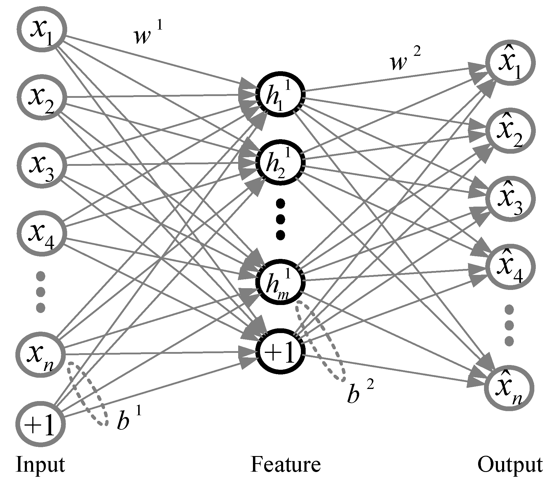
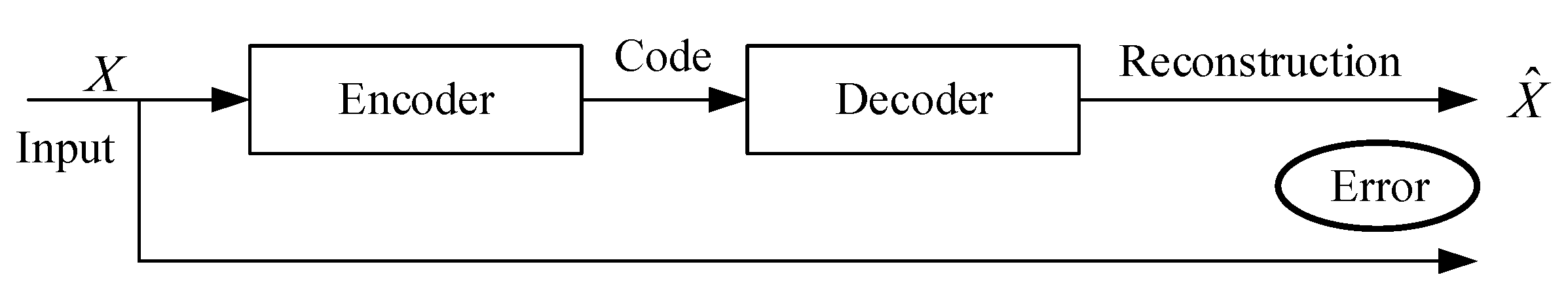
2.2. Framework of Auto-Encoder

Auto-encoder (AE) is a kind of neural network to acquire feature information with the unsupervised learning process. Compared with classical neural networks, AE can extract feature information without teacher data effectively and eliminate dependence on human experience or expertise at facilities diagnosis.

As shown in Figure 2, the output layer vectors have the same dimension with the input layer while minimizing reconstruction error between the input data and the output data. And the input data can be compressed in a hidden layer in which the number of neurons is smaller than that of the input layer.

$$H^{\left(1\right)}={\mathit{f}}_h\left({\mathit{w}}^{\left(1\right)}·\mathit{X}+{\mathit{b}}^{\left(1\right)}\right)$$

(2)

$$\widehat{\mathit{X}}={\mathit{f}}_o\left({\mathit{w}}^{\left(2\right)}{H}^{\left(1\right)}+{\mathit{b}}^{\left(2\right)}\right)$$

(3)

$$minL\left(\theta \right)=\frac{1}{2}\Vert \widehat{\mathit{X}}-\mathit{X}{\Vert }_2^2$$

(4)

$$\theta =\left[{\mathit{w}}^{\left(1\right)},{\mathit{b}}^{\left(1\right)};{\mathit{w}}^{\left(2\right)},{\mathit{b}}^{\left(2\right)}\right]$$

(5)

where $\mathbf{X}=\left(x_1,x_2\cdots x_n\right)$ is the input matrix composed with the raw signal; $H^{\left(1\right)}=\left(h_1^{\left(1\right)},h_2^{\left(1\right)}\cdots h_m^{\left(1\right)}\right)$ is the characteristics of the input data obtained by the encoder process; $\widehat{\mathit{X}}=\left({\widehat{x}}_1,{\widehat{x}}_2\cdots {\widehat{x}}_n\right)$ is the output matrix obtained by the decoder process with hidden output. ${\mathit{w}}^{\left(1\right)}\in {ℝ}^{n\times m}$ and ${\mathit{w}}^{\left(2\right)}\in {ℝ}^{m\times n}$ are the weights between input layer and hidden layer, and between hidden layer and output layer, respectively. In addition, ${\mathit{f}}_h(\cdot )$ and ${\mathit{f}}_o(\cdot )$ are active function that are sigmoid function employed in hidden layer and output layer. The detail description of the feature extraction of the raw signal with AE is shown in the Figure 3.

As shown in Figure 3, the AE learning process mainly divided into encoder process and decoder process, respectively. Firstly, the input data can be compressed by the Equation (2) and obtain the useful features in raw signal. Secondly, the reconstructed signal can be obtained by the decoder process, which can be made comparison with raw signal to determine the performance of AE. Moreover, the performance of the AE learning process is determined with the weights and the bias that can be optimized by minimizing the objective function shown in Equation (4). Finally, the $H^{\left(1\right)}$ treated as the characteristics of raw data is inputted into the next AE for the further learning process.

2.3. Stepwise Intelligent Diagnosis Method Based on SAE

In the case of sliding bearing fault diagnosis, the fault characteristics of contact rubbing (C) and the oil whirl (O) centralize in low frequency in spectrum; the static unbalance (SU) and the dynamic unbalance (DU) centralize in mid-low frequency in spectrum. Moreover, the characteristics in two kinds of unbalance faults are similar, with no obvious boundaries between each other. Therefore, it can be difficult to identify all of them simultaneously to lead to low diagnosis precision. Inversely, if we identify two states in one step, it can effectively reduce the impact from the shortcomings of fault feature and obtain optimal diagnostic accuracy and efficiency. Therefore, a stepwise diagnosis process is proposed and shown in Figure 4, and there are totally four steps in the diagnosis process. Firstly, the signal is divided into normal state (N) and the abnormal state (AN) according to the health condition of the sliding bearing, if the SAE can correctly distinguish the two states (N and AN), the contact rubbing (C) and the other three faults are structured a set of data to distinguish the contact rubbing (C) and the other two faults (OA). If the diagnosis process can be performed successfully, the oil whirl (O) and the unbalance (U) construct a set of data. If the accuracy can meet the requirements of the practical equipment fault diagnosis, we continue to distinguish the static unbalance (SU) and the dynamic unbalance (DU) according to the same method.

The main tool in stepwise intelligent diagnosis method is SAE that is generated by stacking multiple AEs. It is an effective way to imitate the human brain learning process, and it shows great superiority in capturing the representative information from raw signal [24]. The architecture of SAE is shown in the Figure 5.

As shown in Figure 5, the fault feature can be extracted by those AEs and the learned features are inputted into the classifier to perform the fault type identification. In this regard, the greedy layer-wise unsupervised learning is employed to extract better feature representations based on AE, receiving an initial parameters for the first layer, and the output of the first hidden layer is employed (a compressive characterization for the inputted signal) as the input for the next AE, similarly initializing the other AEs. Moreover, the simple architecture of the SAE network training learning process is shown in Figure 6, and the black rectangle is the learned AEs.

As shown in the Figure 6, the output layer of each AE can be removed after finishing the decoder process, remaining a series of cascading models named auto-encoders. Then the successive AEs follow the same transformation conception, and the back-propagation algorithm is applied to globally fine-tune the network parameters to improve the performance of fault diagnosis further. Therefore, SAE is superior to traditional neural network when traditional signal processing method faces with big data contaminated with strong noise, and it can learn the weak features in the raw signal and magnify the useful fault feature information. Therefore, it is suitable to apply to the process of sliding bearing fault diagnosis.

2.4. Proposed Method

Aiming at the limitations of traditional methods for fault diagnosis of rotor system with sliding bearing, a stepwise intelligent diagnosis method based on statistical filter and SAE is proposed for sliding bearing fault diagnosis, which adequately take advantages of the statistical filter to remove the affective of noise and apply SAE to perform stepwise intelligent diagnosis. Moreover, the SAE training process is divided into two phases: unsupervised feature learning and supervised fault identification. The detailed information of the proposed method is described as follows:

• Raw signals of sliding bearing in normal state and 4 kinds of abnormal states using professional experimental platform with sensors;
• Filter noise with the statistical filter between normal state and each abnormal state;
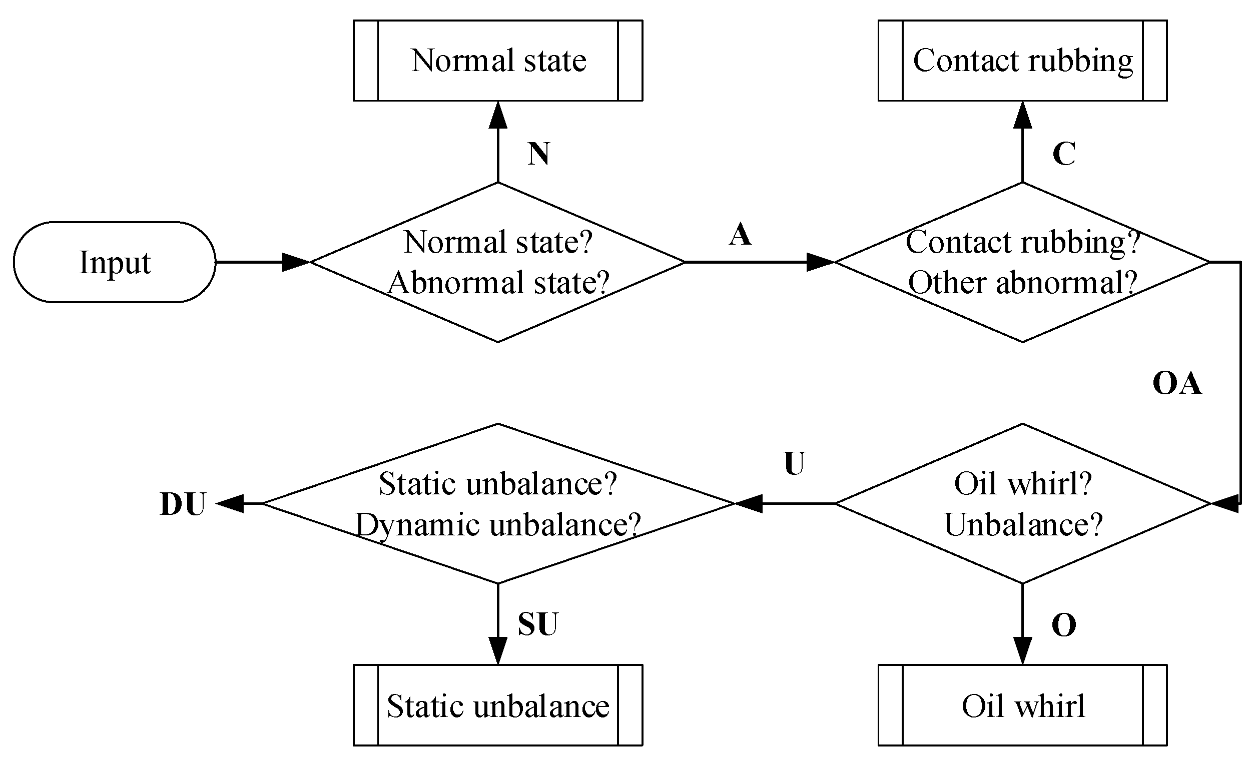
• Decompose five kinds of bearing states into four groups according to Figure 4 and perform the stepwise bearing fault diagnosis with SAE to distinguish two states at each time;
• Establish the deep hierarchical structure with the rule of greedy training, where the auto-encoders are utilized to obtain characteristics of the training sets; output the diagnosis results and stop diagnosis until distinguishing the static unbalance and dynamic unbalance.
• Apply the testing sets to confirm the accuracy of the fault diagnosis with the trained SAE.

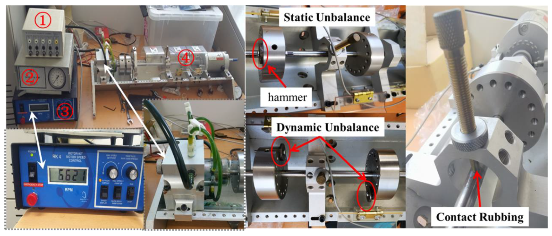
3. Experiment Setup and Data Acquisition

In order to validate the effectiveness and superiority of the proposed method for sliding bearing fault diagnosis, the experimental platform called Bently Nevada rotor kit is shown in Figure 7. The experimental platform is consisted with four parts marked by 1–4 respectively and including data transmitter, oil pump, rotating controller, and rotating device. Therein, a partial enlarged view of part 3 is shown in the lower left corner of Figure 7. When the button on the left in the lower right corner is on the upper side, the rotating speed is set, and the opposite is displayed as the current rotating speed. The middle button is used to change the speed that the upper switch is speeding up quickly, down is speeding reduction. The right button is controller that can determine the state of the experimental platform that is on or off, and the red button is emergency stop button. The oil whirl (O) happens when the rotation frequency is greater than the natural frequency; the static unbalance and dynamic unbalance are physically modeled with horizontal hammers and flanges; the contact rubbing is modeled by the bolt contacting the rotation axis.

Moreover, a partial enlarged view of part 4 is shown in the lower right corner of Figure 7. The right side of the rotating machine is the motor, and the left part is the bearing body that is integrated with the pump. The accelerometer is used to measure the vibration signals of the vertical direction by locating on top of the bearing housing. The sampling frequency is 100 kHz and the sampling time is 10 s. The PCB MA352A60 accelerometers (PCB Piezotronics Inc., Depew, NY, USA) are used to measure the signals of the vertical direction by locating on top of the bearing housing, and they have 10 mV/g sensitivity in the bandwidth from 5 Hz to 60 kHz. The raw signals measured with the accelerometer are transformed into an oscilloscope (Scope Coder DL750) after being magnified by a sensor signal conditioner (PCB ICP Model480C02). Finally, the detailed information of data is described in

Table 1. Introduction of faults in sliding bear.

Rotating Speed	Number	State	Description
5400(RPM)	1,000,000	Normal (N)	/
		Contact rubbing (C)	Bolt contact the rotation axis;
		Oil whirl (O)	Rotation frequency is greater than the natural frequency;
		Static unbalance (SU)	One flange is loaded with 1 hammer with masses of 10 g;
		Dynamic unbalance (DU)	Two flanges are loaded with 2 hammers with masses of 10 g and angle is 180°;

.

4. Results and Discussion

The verification experiment mainly includes three parts. Firstly, the raw signal should be preprocessed by statistical filter and then is reconstructed into the new data to train the SAE model. Secondly, the treated signal is utilized to verify the effectiveness of the proposed method and the signal without statistical filter is also used to make the comparison to explain the necessity of the filter process. Finally, traditional machine learning (BPNN and SVM) and classical deep learning are applied to the fault diagnosis. The results not only proved that SAE is better than traditional neural network in the aspect of the big data for the sliding bearing both effectiveness and accuracy but also it proved that the stepwise intelligent fault diagnosis method can effectively overcome the difficulties that the faults in sliding bearing have no obvious distinguishing features.

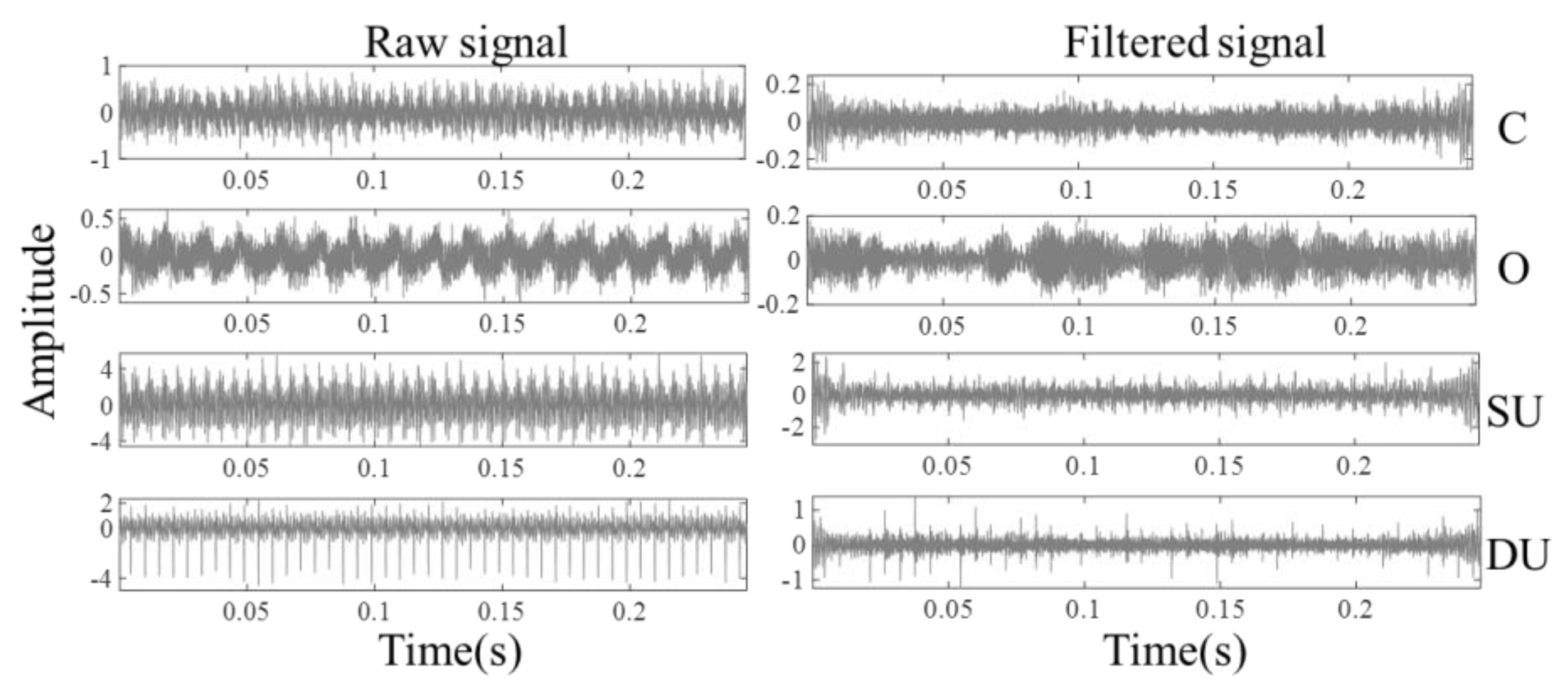
4.1. Data Preprocess with Statistical Filter

The raw signal of sliding bearing is contaminated with intensive background noises due to the characteristic of the abnormal state in the early stage, and it is difficult to ensure the diagnostic efficiency and accuracy. Although deep learning has a strong ability to extract useful information through multiple non-linear transformations and approximate complex non-linear functions with little error [25], it is necessary to filter the signal with the statistical filter according to the quality of the practical signal. The whole process can be described as Figure 8.

As shown in Figure 8, the filter process can be divided into 3 parts. Firstly, the raw signals, including normal signal and one of abnormal signal, are inputted for envelop analysis that is good for the frequency domain transform with FFT. Secondly, the spectrum is divided equally into $M$ parts for statistical filter. In this section, in order to vividly express the experimental results of this filter process, the value of $M$ and SDI in the contact rubbing (C) and unbalance (U) are 1536 and 1.2, respectively; the value of $M$ and SDI in the Oil whirl (O) are 1536 and 0.9, respectively. Moreover, the total number of the data is 24,576 (about 0.24576 s) as an example, and the length of each part is 16 since it is the power exponent of 2. Thirdly, the filter process is performed as shown in Figure 8 and the result is described in Figure 9. It can be seen that the noise in the raw signal can be removed though the statistical filter and the filtered signal can be treated as the input data for the stepwise intelligent fault diagnosis based on SAE to perform fault diagnosis with high precision and efficiency.

4.2. Stepwise Intelligent Fault Diagnosis Based on SAE

In this section, the experimental data arrangement and the learning process are introduced to describe the fault diagnosis process vividly. The effectiveness and feasibility of the proposed method is proved through applying it to a practical platform for sliding bearing fault diagnosis.

4.2.1. Description of Data in Stepwise Process

The data of stepwise diagnosis process is arranged as

Table 2. Description of experimental data.

No.	Group 1	Group 2
1	N (983,040)	C+O+SU+DU; (each state is 245,760)
2	C (983,040)	O+SU+DU; (each state is 327,680)
3	O (983,040)	SU+DU; (each state is 491,520)
4	SU (983,040)	DU (each state is 983,040)

according to the Figure 4 to distinguish two states at once. Moreover, the experimental data is preprocessed by statistical filter and then is reconstructed into the train data and the test data.

• There are five kinds of sliding bearing signal (normal state, contact rubbing, oil whirl, static unbalance, and dynamic unbalance) in this experiment and they are one-dimension data whose length is 1,000,000; moreover, the statistical filter is utilized to filter the noise and obtain the new data that marked as normal state $N_{\mathrm{983,040}\times 1}^{\prime }$, contact rubbing $C_{\mathrm{983,040}\times 1}^{\prime }$, oil whirl $O_{\mathrm{983,040}\times 1}^{\prime }$, static unbalance $S{U}_{\mathrm{983,040}\times 1}^{\prime }$ and dynamic unbalance $D{U}_{\mathrm{983,040}\times 1}^{\prime }$;
• The data can be reconstructed into a matrix and the number of rows of the matrix is 8192 (2¹³ = 8192), and it fully contains the amount of data generated by one rotation of the sliding bearing; the column of the matrix change with the stepwise intelligent diagnosis to keep same size of two groups (two states of bearing). For example, the length of the contact rubbing state is 983,040 (8192 × 120), and the other three states are 327,680 (8192 × 40); similarly, the length of the oil whirl state is 983,040 (8192 × 120), and the other two states are 491,520 (8192 × 60);
• Two sets of data (group1 and group2) in stepwise fault diagnosis are marked as $G_{8192\times 120}^1$ and $G_{8192\times 120}^2$. The train data $G_{train}^1$ (100 × 8192) is above 80% in the first half of $G^1$ and similarly $G_{train}^2$ (100 × 8192) is also above 80% in the first half of $G^2$ and the remaining data is test data. Therefore, the train data and the test data in this experiment are $X_{train}=\left[G_{train}^{\prime 1};G_{train}^{\prime 2}\right]$ (200 × 8192) and $X_{test}=\left[G_{test}^{\prime 1};G_{test}^{\prime 2}\right]$ (40 × 8192), respectively;
• The data labels are marked as [0, 1] according to the group 1 and group 2, respectively. Then the label data are expanded to vectors according to $X_{train}$ and $X_{test}$ and they are marked as $Y_{train}$ (200 × 1) and $Y_{test}$ (40 × 1). Therein, the first half of the vectors is 0 and remaining values are 1.

4.2.2. Process of SAE Learning

The SAE learning is mainly divided into unsupervised feature extraction (information compression) stage and supervised state identification stage. Furthermore, there are totally four AEs, and each hidden layer of proposed method utilized in this case is consists of 4000, 2000, 500, and 30 neuroses, respectively. The learning rate and momentum of each AE are 0.9 and 0.5, respectively. The active function is the ‘sigmoid’. Moreover, the input layer consists of 8192 neuroses representing the 8192-dimension, and the output layer has one neuron representing bearing state (0 or 1). The detailed parameters of the proposed method are described in

Table 3. Detailed information of SAE.

No. of Hidden Layers	No. of Neurons in Hidden Layer	No. of Iterations
4	4000-2000-500-30	2000
Learning rate	Momentum	Masked fraction
0.9	0.5	0

.

There are five parts in the stepwise intelligent diagnosis of the sliding bearing for rotor system. Firstly, the train data $X_{train}$ is sequentially assigned to the AEs (from AE-1 to AE-4) to complete the feature extraction. Secondly, the extracted feature is putted into the neural network, which includes the compressed feature in hidden layer and the weights of the four AEs. Thirdly, the gradient descent is utilized to globally fine-tune the weights between the layers according to the $Y_{train}$. Finally, the $X_{test}$ and $Y_{test}$ are applied to verify the accuracy of the fault diagnosis. The pseudocode of the stepwise intelligent fault diagnosis is shown as

Table 4. Pseudocode of the stepwise intelligent fault diagnosis.

Input: Output:	The 5 Kinds of Sliding Bearing Signal Bearing Fault Diagnosis Result
/*Raw signal preprocessed*/
The raw signal preprocessed with statistical filter and obtain new signal $N^{\prime }$, $C^{\prime }$, $O^{\prime }$, $S{U}^{\prime }$, $D{U}^{\prime }$;
/*SAE training process*/
Construct data according to Table 2 and obtain $G^1$ and $G^2$;
Mark label data as [0,1] according to $G^1$, $G^2$;
Divide the train data $X_{train}$ and $Y_{train}$; and test data $X_{test}$, $Y_{test}$;
/Auto-encoder (Unsupervised learning)/
Construct AE-1, AE-2, AE-3 and AE-4;   Obtain $H_1$ and $W_1$ by inputting the train data ($X_{train}$) to AE-1(8192-4000-8192);
Obtain $H_2$ and $W_2$ by inputting $H_1$ to AE-2 (4000-2000-4000);
Obtain $H_3$ and $W_3$ by inputting $H_2$ to AE-3 (2000-500-2000);
Obtain $H_4$ and $W_4$ by inputting $H_3$ to AE-4 (500-30-500);
/Network classification process (supervised learning)/
Build a neural network architecture: 8192-4000-2000-500-30-1;
Enter $H_1$, $H_2$, $H_3$, $H_4$ and $W_1,W_2,W_3,W_4$ into the network to initialize parameters;   Assign output layer weight $W_5$ randomly and obtain the actual output $Y$;
Perform the gradient descent to fine-tune the globally $W_1,W_2,W_3,W_4,W_5$;
Get SAE training model;
/*SAE testing process*/
The test data $X_{test}$ is substituted into the above-mentioned trained classification model for fault identification, and the identification results are outputted and compared with $Y_{test}$.

.

4.2.3. Validation Results

Furthermore, the experimental result of the proposed method for sliding bearing is shown as Figure 10, when the parameter of SAE is setting as Table 3. As shown in Figure 10, all the data is correctly classified and there are no samples to be misclassified. Therefore, it can achieve a diagnosis of 100% and prove the effectiveness and feasibility of the proposed method in the fault diagnosis of sliding bearing. Also, the results of comparative experiments using the raw signal without statistical filter or stepwise diagnosis are collected in

Table 5. Results of comparative experiments based on SAE.

	Method A	Method B	Method C
Accuracy	85%	62.5%	25%
Standard deviation	0.1045	1.0085	2.3574

.

In Table 5, the method A is representing the proposed method without the statistical filter, the method B is representing the proposed method without the stepwise diagnosis and the method C is representing that the SAE is only utilized to perform the fault diagnosis of the sliding bearing with the raw signal in time domain. The parameters of the neural network (SAE) are same as the Table 3. Moreover, the result is the mean value of 10 trails to guarantee the statistical validity of experimental results.

The results described as Table 5 prove that the proposed method not only releases the manual labor and the dependence on professional knowledge but also accurately identifies faint and weak features between multiple faults in sliding bearings. Moreover, it can be found that the standard deviation of the method C is the 2.3574 that is the biggest in the three methods since the noise in signal is deceptive in the process of accurately identifying the bearing in the neural network. Therefore, the proposed method can give full play to the statistical filter and stepwise diagnosis to overcome the difficulties, including noise and complex features in the process of fault diagnosis.

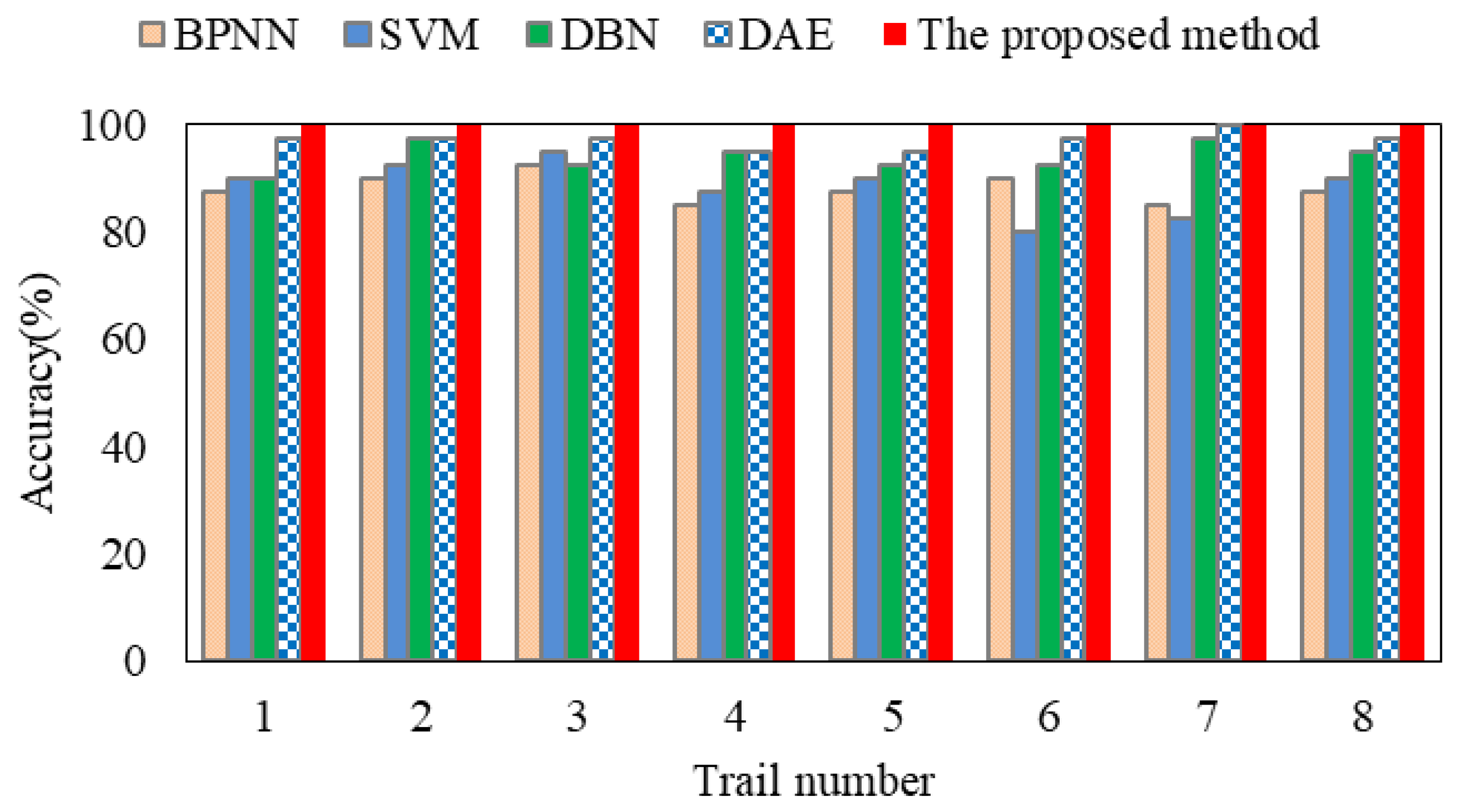
5. Comparative Experiment

In order to further demonstrate the superiority of the proposed method in sliding bearing fault diagnosis, another commonly used fault diagnosis methods, such as the BPNN, SVM, deep belief networks (DBN), and denoising autoencoder (DAE) are applied for comparison. The parameters in BPNN and SVM are shown in

Table 6. Parameters of SVM and BPNN.

Method	No. of Hidden Layers	No. of Neurons in Hidden Layer	No. of Iterations
BPNN	3	7-12-1	1000
SVM	Function		Type of SVM
	sigmoid kernel function		epsilon-SVR

. Moreover, the type of SVM is set to be epsilon-SVR, and sigmoid kernel function is used. Also, the parameters of DBN are collected in

Table 7. Parameters of DBN and DAE.

Method	No. of Hidden Layers	No. of Neurons in Hidden Layer	No. of Iterations
DBN	4	4000-2000-500-30	2000
	Learning Rate	Momentum	$\mathsf{\alpha }$
	0.9	0.5	1
DAE	No. of Hidden Layers	No. of Neurons in Hidden Layer	No. of Iterations
	4	4000-2000-500-30	2000
	Learning Rate	Momentum	Masked Fraction
	0.9	0.5	0.5

. The parameters of DAE have the same setting with the stepwise intelligent fault diagnosis based on SAE, and the only difference is that masked fraction is set to 0.5 (this parameter in SAE is setting to 0) to denoise. The sigmoid function [26] is selected as active function for the BPNN, DAE, and DBN, the optimizing search algorithms for adjusting the parameters of those neural networks is the traditional gradient descent [27]. Meanwhile, both DBN and DAE directly handle the raw signals, whereas the signal is without statistical filter and stepwise diagnosis. The experimental data in the classical deep learning is the raw signal translated with the FFT.

The train data of the BPNN and SVM is the feature parameters in frequency domain is displayed in

Table 8. Feature parameters in frequency domain.

Parameter ($f_i$ is Frequency (Hz) and $F\left(f_i\right)$ is the Frequency Transformation)

$P_1=\sqrt{({{\displaystyle \sum }}_{i=1}^I{f}_i^2\cdot F\left(f_i\right))/{{\displaystyle \sum }}_{i=1}^{I}F\left(f_i\right)}$; $P_2=\sqrt{({{\displaystyle \sum }}_{i=1}^I{f}_i^4\cdot F\left(f_i\right))/{{\displaystyle \sum }}_{i=1}^I{f}_i^{2}F\left(f_i\right)}$

$P_3={{\displaystyle \sum }}_{i=1}^I{f}_i^2\cdot F\left(f_i\right)/{\left({{\displaystyle \sum }}_{i=1}^{I}F\left(f_i\right){{\displaystyle \sum }}_{i=1}^I{f}_i^{4}F\left(f_i\right)\right)}^{\frac{1}{2}}$

$P_4=\sigma /\overline{f}$;$\overline{f}={{\displaystyle \sum }}_{i=1}^I{f}_i\cdot F\left(f_i\right)/{{\displaystyle \sum }}_{i=1}^{I}F\left(f_i\right)$;$\mathsf{\sigma }=\sqrt{{{\displaystyle \sum }}_{i=1}^I{\left(f_i-\overline{f}\right)}^2\cdot F\left(f_i\right)/I}$

$P_5={{\displaystyle \sum }}_{i=1}^I{\left(f_i-\overline{f}\right)}^3\cdot F\left(f_i\right)/\left({\sigma }^3\cdot I\right)$; $P_6={{\displaystyle \sum }}_{i=1}^I{\left(f_i-\overline{f}\right)}^4\cdot F\left(f_i\right)/\left({\sigma }^4\cdot I\right)$

$P_7={{\displaystyle \sum }}_{i=1}^I\sqrt{\left(f_i-\overline{f}\right)}\cdot F\left(f_i\right)/\left(\sqrt{\sigma }\cdot I\right)$

. The 7 feature parameters in frequency are average characteristic frequency, frequency of closing the time average per-unit time, waveform stability index, rate of change, skewness, kurtosis, and sum of power spectra, respectively. The BPNN has three layers, which consists of input layer, hidden layer, output layer and the numbers of neurons are 7, 12, and 1, respectively. Finally, the detailed testing accuracy of 4 methods is shown in Figure 11.

As shown in Figure 11, the performance of the DBN and DAE is better than those of the SVM and BPNN with the seven feature parameters, regardless whether the signals are preprocessed or not. It can fully validate the ability of deep learning methods with deep architectures for automatically extracting discriminative features. Moreover, it found that the proposed method can obtain better results than the DBN and DAE even when they have deep architectures. These reasons fully validate the necessity of the stepwise intelligent fault diagnosis for the sliding bearing since the feathers of different faults are ambiguous. In addition, they can illustrate the superiority of the statistical filter of the proposed method in learning more sensitive features that are useful for classification by comparing the DAE; even the DAE has the best performance in the four methods in Figure 11.

6. Conclusions

Stepwise intelligent diagnosis method is proposed in this paper for a rotor system based on statistical filter and SAE. The raw signals were pre-processed by statistical filter to get denoised signal as the input data for SAE that is better to learn more useful feature automatically from signal. The proposed method is performed to distinguish the key features between five different healthy conditions of the sliding bearing correctly. The fault diagnosis case with sliding bearing successfully demonstrates the effectiveness and the feasibility of the proposed method. Moreover, the comparative experiments also validate the advantages of the proposed method with other intelligent methods.

References

1. Guo, M.; Li, W.; Yang, Q.; Zhao, X.; Tang, Y. Amplitude filtering characteristics of singular value decomposition and its application to fault diagnosis of rotating machinery. Measurement 2020, 154, 107444. [Google Scholar] [CrossRef]
2. Zernin, M.V.; Mishin, A.V.; Rybkin, N.N.; Shil’Ko, S.V.; Ryabchenko, T.V. Consideration of the multizone hydrodynamic friction, the misalignment of axes, and the contact compliance of a shaft and a bush of sliding bearings. J. Frict. Wear 2017, 38, 242–251. [Google Scholar] [CrossRef]
3. Vincent, B.; Maspeyrot, P.; Frêne, J. Cavitation in noncircular journal bearings. Wear 1997, 207, 122–127. [Google Scholar] [CrossRef]
4. Yan, X.; Liu, Y.; Zhang, W.; Jia, M.; Wang, X. Research on a Novel Improved Adaptive Variational Mode Decomposition Method in Rotor Fault Diagnosis. Appl. Sci. 2020, 10, 1696. [Google Scholar] [CrossRef] [Green Version]
5. Yu, X.; Dong, F.; Ding, E.-J.; Wu, S.; Fan, C. Rolling Bearing Fault Diagnosis Using Modified LFDA and EMD with Sensitive Feature Selection. IEEE Access 2018, 6, 3715–3730. [Google Scholar] [CrossRef]
6. Shi, J.; Du, G.; Ding, R.; Zhu, Z. Time Frequency Representation Enhancement via Frequency Matching Linear Transform for Bearing Condition Monitoring under Variable Speeds. Appl. Sci. 2019, 9, 3828. [Google Scholar] [CrossRef] [Green Version]
7. Xu, Y.; Cai, Z.; Ding, K. An enhanced bearing fault diagnosis method based on TVF-EMD and a high-order energy operator. Meas. Sci. Technol. 2018, 29, 095108. [Google Scholar] [CrossRef]
8. Song, L.; Wang, H.; Chen, P. Vibration-Based Intelligent Fault Diagnosis for Roller Bearings in Low-Speed Rotating Machinery. IEEE Trans. Instrum. Meas. 2018, 67, 1887–1899. [Google Scholar] [CrossRef]
9. Song, L.; Wang, H.; Chen, P. Step-by-Step Fuzzy Diagnosis Method for Equipment Based on Symptom Extraction and Trivalent Logic Fuzzy Diagnosis Theory. IEEE Trans. Fuzzy Syst. 2018, 26, 3467–3478. [Google Scholar] [CrossRef]
10. Glowacz, A. Acoustic fault analysis of three commutator motors. Mech. Syst. Signal Process. 2019, 133, 106226. [Google Scholar] [CrossRef]
11. Zhao, H.; Zheng, J.; Xu, J.; Deng, W. Fault Diagnosis Method Based on Principal Component Analysis and Broad Learning System. IEEE Access 2019, 7, 99263–99272. [Google Scholar] [CrossRef]
12. Agrawal, P.; Jayaswal, P. Diagnosis and Classifications of Bearing Faults Using Artificial Neural Network and Support Vector Machine. J. Inst. Eng. (India) Ser. C 2019, 101, 61–72. [Google Scholar] [CrossRef]
13. Zhang, K.; Yang, Z. Identification of Load Categories in Rotor System Based on Vibration Analysis. Sensors 2017, 17, 1676. [Google Scholar] [CrossRef] [PubMed] [Green Version]
14. Deng, H.; Diao, Y.; Wu, W.; Zhang, J.; Ma, M.; Zhong, X. A high-speed D-CART online fault diagnosis algorithm for rotor systems. Appl. Intell. 2019, 50, 29–41. [Google Scholar] [CrossRef]
15. Wang, D.; Zhao, X.; Kou, L.-L.; Qin, Y.; Zhao, Y.; Tsui, K.-L. A simple and fast guideline for generating enhanced/squared envelope spectra from spectral coherence for bearing fault diagnosis. Mech. Syst. Signal Process. 2019, 122, 754–768. [Google Scholar] [CrossRef]
16. Li, X.; Zhang, W.; Ding, Q.; Sun, J.-Q. Multi-Layer domain adaptation method for rolling bearing fault diagnosis. Signal Process. 2019, 157, 180–197. [Google Scholar] [CrossRef] [Green Version]
17. Krolczyk, G.M.; Li, Z.; Antonino-Daviu, J.A. Fault Diagnosis of Rotating Machine. Appl. Sci. 2020, 10, 1961. [Google Scholar] [CrossRef] [Green Version]
18. Li, C.; Zhang, W.; Peng, G.; Liu, S. Bearing Fault Diagnosis Using Fully-Connected Winner-Take-All Autoencoder. IEEE Access 2017, 6, 6103–6115. [Google Scholar] [CrossRef]
19. Yuan, Z.; Zhang, L.-B.; Duan, L. A novel fusion diagnosis method for rotor system fault based on deep learning and multi-sourced heterogeneous monitoring data. Meas. Sci. Technol. 2018, 29, 115005. [Google Scholar] [CrossRef]
20. Jia, F.; Lei, Y.; Lin, J.; Zhou, X.; Lu, N. Deep neural networks: A promising tool for fault characteristic mining and intelligent diagnosis of rotating machinery with massive data. Mech. Syst. Signal Process. 2016, 72, 303–315. [Google Scholar] [CrossRef]
21. Oh, H.; Jung, J.H.; Jeon, B.C.; Youn, B.D. Scalable and Unsupervised Feature Engineering Using Vibration-Imaging and Deep Learning for Rotor System Diagnosis. IEEE Trans. Ind. Electron. 2018, 65, 3539–3549. [Google Scholar] [CrossRef]
22. Li, K.; Chen, P.; Wang, S. An Intelligent Diagnosis Method for Rotating Machinery Using Least Squares Mapping and a Fuzzy Neural Network. Sensors 2012, 12, 5919–5939. [Google Scholar] [CrossRef] [PubMed] [Green Version]
23. Liao, Z.; Song, L.; Chen, P.; Zuo, S. An automatic filtering method based on an improved genetic algorithm—with application to rolling bearing fault signal extraction. IEEE Sens. J. 2017, 17, 1. [Google Scholar] [CrossRef]
24. Wu, Z.; Jiang, H.; Zhao, K.; Li, X. An adaptive deep transfer learning method for bearing fault diagnosis. Measurement 2020, 151, 107227. [Google Scholar] [CrossRef]
25. Li, X.; Zhang, W.; Ding, Q. Understanding and improving deep learning-based rolling bearing fault diagnosis with attention mechanism. Signal Process. 2019, 161, 136–154. [Google Scholar] [CrossRef]
26. Rao, M.; Li, Q.; Wei, D.; Zuo, M.J. A deep bi-directional long short-term memory model for automatic rotating speed extraction from raw vibration signals. Measurement 2020, 21, 107719. [Google Scholar] [CrossRef]
27. Zhao, W.; Hua, C.; Dong, D.; Ouyang, H. A Novel Method for Identifying Crack and Shaft Misalignment Faults in Rotor Systems under Noisy Environments Based on CNN. Sensors 2019, 19, 5158. [Google Scholar] [CrossRef] [Green Version]
Figure 1. Process of the statistical filter.
Applsci 10 02477 g001
Figure 2. Conceptual diagram of the auto-encoder.
Applsci 10 02477 g002
Figure 3. Detailed description of auto-encode (AE).
Applsci 10 02477 g003
Figure 4. Stepwise diagnosis process.
Applsci 10 02477 g004
Figure 5. Brief architecture of SAE network.
Applsci 10 02477 g005
Figure 6. Brief sketch of SAE.
Applsci 10 02477 g006
Figure 7. Experimental platform of sliding bearing.
Applsci 10 02477 g007
Figure 8. Detailed information for filter process.
Applsci 10 02477 g008
Figure 9. Experimental results with statistical filter.
Applsci 10 02477 g009
Figure 10. Fault classification of the proposed method, there are four steps in the fault diagnosis process.
Applsci 10 02477 g010
Figure 11. Comparative experiments of four methods.
Applsci 10 02477 g011