Abstract
The output torque is an important performance indicator of a motor. Due to the special structure of a permanent magnet spherical motor (PMSM), it is difficult to measure its torque. This paper proposes a novel method to measure the output torque of the PMSM. The proposed method uses the microelectromechanical system (MEMS) gyroscope to measure the rotor motion acceleration, which is then used to calculate the output torque based on the rotor dynamics equation. In this paper, we firstly simulate and analyze the output torque of the PMSM. Secondly, we design a torque-measuring device to measure the output torque. Thirdly, we compare and discuss the experimental and simulation results. The comparison results show that the proposed method is feasible.
1. Introduction
In recent years, with the development of industrial automation and the progress of science and technology, multi-degree-of-freedom (multi-DOF) motors are more demanded in aerospace, intelligent transportation, medical and industrial robots, and other industrial applications [1]. A traditional multi-DOF motion system, which consists of multiple single-DOF motors and transmission mechanical structure [2], has the problems of low reliability, low efficiency and high energy consumption [3,4]. To solve the above-mentioned problems, a permanent magnet spherical motor (PMSM), which is a kind of multi-DOF motor, has been developed and has attracted attention from researchers and practitioners.
Output torque is one of the essential performance indicators to evaluate the performance of the PMSM. However, output torque measurement is difficult in the research of PMSM. Many researchers have proposed methods to measure the output torque of PMSM at different structures. In the work of [5,6], a torque measurement system is designed with a pressure sensor mounted in a torsion cantilever bracket structure. In [7,8], a torque measurement system with a torque sensor installed in the circular and curved-guide rail is designed for different PMSMs. Moreover, for an inductive spherical motor, an output torque measurement system consists of a brushless motor and a six-axis force sensor installed on the rotor ball, is developed in the papers [9,10]. In [11], a tension meter is utilized to measure the cogging torque of a spherical motor, based on the principle of the torque balance method. So far, the above methods for torque measurement are specially developed for the existing structures of PMSMs, which lack of generality. Furthermore, these measurement systems have complex structures and low maintainability, and can only measure the static torque in the form of spin motion. These methods are not proper for the PMSM in this paper and cannot be directly applied for the torque measurement.
In this paper, the output torque of a 3-DOF PMSM is simulated and experimentally studied by considering friction loss and other factors of the inclined mode of excitation current. A MEMS gyroscope sensor is utilized to measure the rotor angular acceleration, which is then used to calculate rotor output torque on the basis of rotor dynamics equation for PMSMs. Simultaneously, the finite element simulation is used to analyze the magnetic field distribution of the PMSM, and then the automatic dynamic analysis of mechanical systems (ADAMS) is conducted for the mechanical simulation. By comparing and analyzing the simulation results with the experimental data collected by the MEMS gyroscope sensor, it is found that the output torque of the simulation is larger than that measured in the experiment because the friction is neglected in the simulation. The analysis results verify the feasibility of the proposed torque measurement for PMSMs.
2. Electromagnetic Theory and Simulation of the Output Torque of a Spherical Motor
2.1. Motor Structure
This paper studies a 3-DOF PMSM, which is mainly composed of a stator spherical shell, stator coils, a rotor spherical shell, rotor permanent magnets, and a rotor output shaft [12,13,14]. In the PMSM, the upper and lower hemispheric shells of the stator of the spherical motor are evenly arranged with 12 copper coils without the iron core. The latitude angle between the stators on the upper and lower spherical shells is 45 degrees, and the longitude angle between the adjacent stators is 30 degrees. The spherical surface of the rotor is inlaid with 40 NdFeB permanent magnets. The N and S pole magnets are distributed along the warp and weft directions. The latitude angle between the upper and lower adjacent permanent magnet is 30 degrees. The longitude angle between the left and right adjacent permanent magnets is 36 degrees. The structure of the stator and rotor is shown in Figure 1.
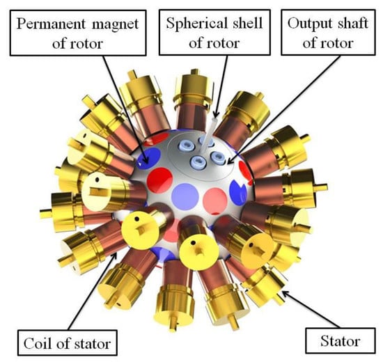
Figure 1.
Structure of the stator and rotor.
2.2. Electromagnetic Theory of Output Torque
Electromagnetic torque of the PMSM can be theoretically analyzed by using the finite element method (FEM) and virtual displacement principle [15,16]. The current through coils is assumed to be constant and the motor is considered to be an ideal system without the loss of energy. Then, the change in electrical energy as an input into the PMSM will be converted partly into the change in magnetic field energy , and partly into the change in mechanical energy . If the current is constant, the change in the electrical energy can be ignored and we obtain
According to the relationship between energy and torque, when the rotor rotates at a small angle , its torque can be expressed as:
The magnetic field energy of the system in the whole solution region can be obtained as follows:
where is the magnetic field intensity and is the magnetic flux intensity.
In order to simplify the electromagnetic analysis of the PMSM, which has multiple permanent magnets in the stator and coils in the rotor, the electromagnetic torque generated by the interaction of a single rotor permanent magnet and a single stator coil is firstly analysed. For a single pair of the permanent magnet and coil, the electromagnetic torque can be obtained as:
where represents the deflection angle of the i-th coil relative to the j-th stator permanent magnet, and represents the electromagnetic torque generated by a single pair of the permanent magnet and coil. is a characteristic function achieved by the FEM and describes the relationship between the electromagnetic torque and the deflection angle when the coil is energized by the unit current. represents the ampere-turns of the coil, and represent the position vector of the i-th stator coil and the i-th rotor permanent magnet, respectively. According to the principle of superposition, the total torque vector is obtained as follows:
2.3. Torque Simulation
In order to calculate the magnetic field and electromagnetic torque by the FEM, a three-dimensional finite element simplified model of the PMSM is established according to its structural characteristics and is shown in Figure 2. In the simulation model, the right hand reference coordinate system OXYZ is established, and the position of the centre of the spherical motor stator is set as the origin O of the coordinate system. The Z axis passing through the origin O is perpendicular to the XOY plane and pointing in the direction of the vertical upward direction.
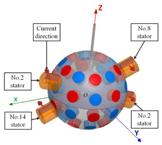
Figure 2.
Simulation Model.
The direction of the cross-section current of the stator coil is set according to the direction indicated by the red arrow in Figure 2, so that the S pole of the coil faces the surface of the rotor. To compare the simulation results with the experimental ones, the simulation current parameters are set as same as the measured current, as shown in Table 1. The total current applied to the coil starts from 1.45 A, increasing by about 0.3 A at every interval, and finally reaches 5.42 A. The meshes of stator and rotor for the PMSM simulation model are shown in Figure 3.

Table 1.
Current value of stator coil excitation source.
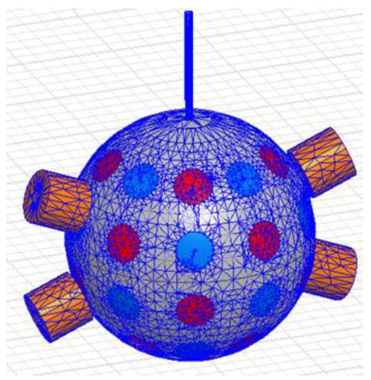
Figure 3.
Meshes of stator and rotor.
The Neumann boundary conditions are applied to the simulation model. As shown in Figure 4, the magnetic field line does not cross the boundary under this setting. Figure 5 shows the simulation results of the output torque of the PMSM. It can be seen that the magnitude of the simulated torque increases slowly and is approximately linear with the increase of current. The total current of the coils increases by every 1 A, the torque increases by about 115 mN·m. This indicates that the output torque is proportional to the current of the stator coil under this power-on strategy.
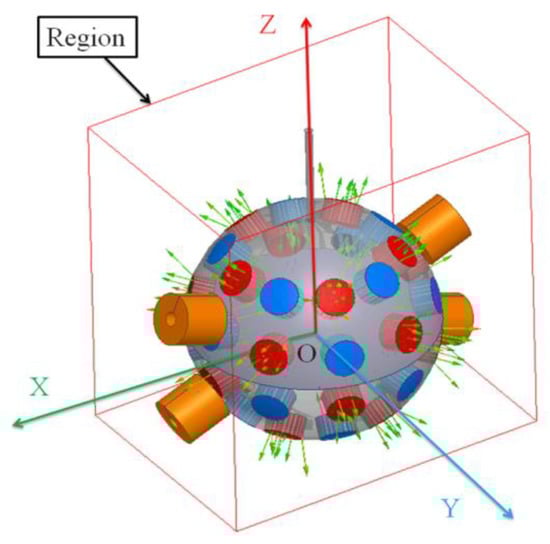
Figure 4.
Boundary settings of stator and rotor.
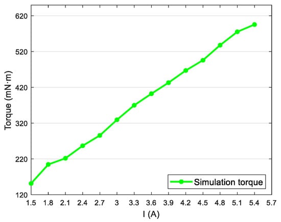
Figure 5.
Simulated torque with the increase of current.
3. Experimental Test of Output Torque for a PMSM
3.1. Experimental Setup
The test platform to measure output torque of the PMSM is shown in Figure 6. It mainly consists of a drive circuit, a control circuit, a computer, and a MEMS gyroscope sensor. The MPU6050 is chosen as the core component of the MEMS gyroscope sensor and is used to obtain rotor dynamics data which is then processed by the computer.
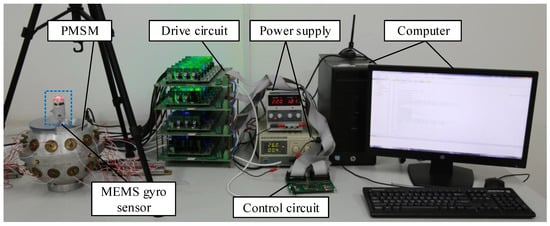
Figure 6.
Test platform for torque measurement.
Figure 7 shows the installation location of the MEMS gyroscope sensor and the initial position of the rotor in the experiment. The MEMS gyroscope sensor is mounted on the top of the output shaft as shown in Figure 7a. As shown in Figure 7b, the demo board containing MPU6050 is placed inside the sensor housing. The sensor housing is mounted on the top of the output shaft and two screws are used to hold it in place. The reset key of the demo board is on the sensor housing. When the rotor is adjusted to the initial position, the reset key will be pressed to avoid drift errors and to ensure that the current position is the initial position for the sensor. The initial position of the rotor shown in Figure 7c is a relative position between the rotor and the stator, which is consistent with that in the coordinate system of the simulation model in Figure 2. A detachable limit device shown in Figure 7b is utilized to ensure that the rotor can be adjusted to the initial position before the experiment is conducted. The stator static coordinate OXYZ is coincided with the simulation coordinate. When the PMSM is driven, the relevant dynamic data are measured by the MEMS gyro sensor and are kept in the computer.
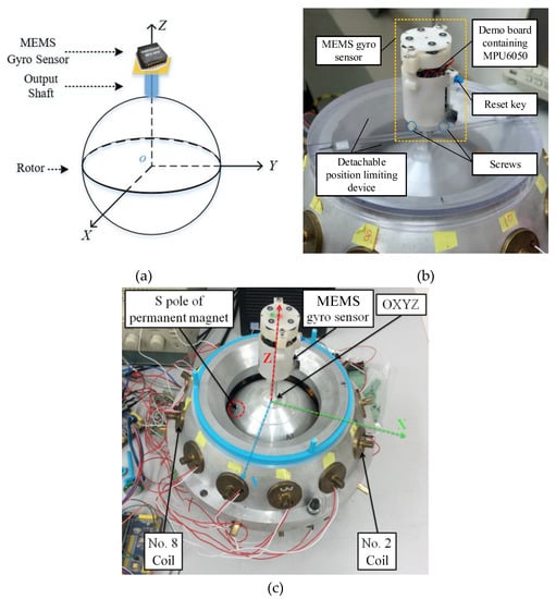
Figure 7.
Installation of the MEMS gyroscope sensor: (a) The installation diagram; (b) The MEMS gyroscope sensor; (c) The initial position.
In the experiment, the oscilloscope was connected to the AC/DC current probe of A622 100 Amp type and then used to monitor the current of each coil winding. The PWM current waveform of No. 2 stator coil with a duty cycle of 90% is shown in Figure 8, and the measured current data are shown in Table 1.
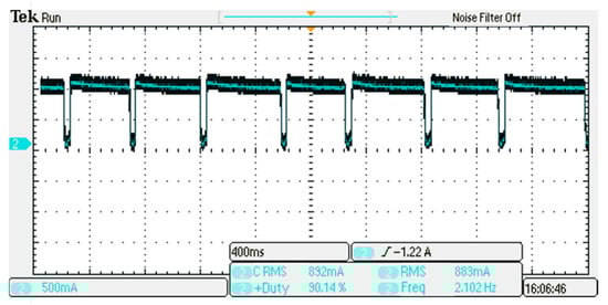
Figure 8.
Current of No. 2 stator coil.
3.2. Principles of Experimentation
The coordinate system OpXpYpZp of the rotor is defined as a reference to describe the position of the rotor. It is a right-hand dynamic coordinate system. The origin O is always coincident with the origin of the stator coordinate system OXYZ, which is defined in Figure 2. As shown in Figure 9, the coordinate system OXYZ is coincident with OpXpYpZp when the rotor does not rotate.
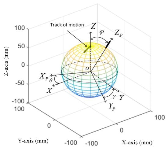
Figure 9.
The motion trajectory in the measurement coordinate system.
When the rotor of the PMSM is moving to one direction, without considering friction force its dynamics can be expressed according to Lagrange’s Equations of second kind [17,18], and its output torque can be derived as follows:
where is the output torque vector of the PMSM. is the rotor angular displacement vector; is the rotor inertia matrix. is the Gothic and centrifugal force matrix and can be ignored under the condition of rotation around the constant axis. is denoted as:
where , and are the moments of inertia that are relative to each coordinate axis of OXYZ. Substituting Equation (8) into Equation (7) the relationship between the output torque and the rotor angular acceleration is expressed as:
, and are rotor angular acceleration components decomposed into X-, Y-, Z-axis, respectively. Moreover, the rotor angular acceleration vector can be expressed as . Obviously, can be obtained if the moment of inertia and angular acceleration vector can be measured on the basis of the known rotor material, size and structure. The moments of inertia can be calculated by using the ADAMS software. The simulation results of the moment of inertia of each coordinate axis in the coordinate system are respectively obtained as , , .
The remaining challenge is to obtain the components of rotor angular acceleration , , and using the dynamic information obtained by the MEMS gyroscope sensor. Define , and as components of the unit position vector of the rotor on each coordinate axis of OXYZ. represents the time sequence number of the rotor position vector that is collected by the sensor, and represents the sampling time. By using the MPU6050 gyroscope sensor, the components , , and can be measured during the sampling time [19]. The formula for calculating , , and via Euler angles can be obtained as follows:
where , , , and are Euler angles shown in Figure 9.
Based on the definition of linear velocity, the components of unit linear velocity vector , , and during the i-th sampling time are obtained by taking the first derivative of , , and as follows:
where .
Similarly, based on the definition of linear acceleration, the components of unit linear acceleration vector , , and during the i-th sampling time are obtained by taking the first derivative of , , and as follows:
where .
In the three-dimensional space, angular acceleration vector in the fixed coordinate system OXYZ is expressed according to the rigid body kinematics as follows:
where is the rotor position vector, is the rotor linear acceleration, represents cross product. According to the definition of the unit position vector and unit linear acceleration vector in Equation (9) and Equation (11), it can be obtained that:
where , . By taking Equation (13) into Equation (12), the angular acceleration is rewritten as follows:
Furthermore, the components of during the i-th sampling time are derived as:
By taking Equation (9), (10), and (11) into Equation (15), the functional relation of the angular acceleration vector and Euler angles can be established as Equation (16).
The flow chart for calculating the output torque is shown in Figure 10.
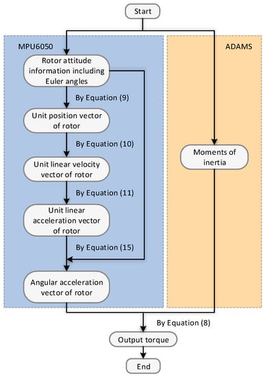
Figure 10.
Flow chart for calculating output torque.
3.3. Experimental Results
As shown in Figure 9, under the condition that the stator winding current is set as 5.42 A, the computer draws the trajectory diagram of the tilt motion mapped on the sphere with a radius of 65 mm. The corresponding components of the unit linear velocity vector, unit linear acceleration vector, angular acceleration and output torque vector in the stator coordinate system OXYZ, are shown in Figure 11, Figure 12, Figure 13 and Figure 14, respectively.
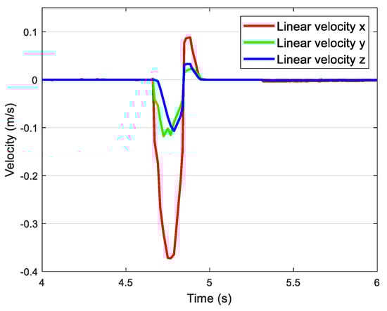
Figure 11.
Components of the unit linear velocity vector.
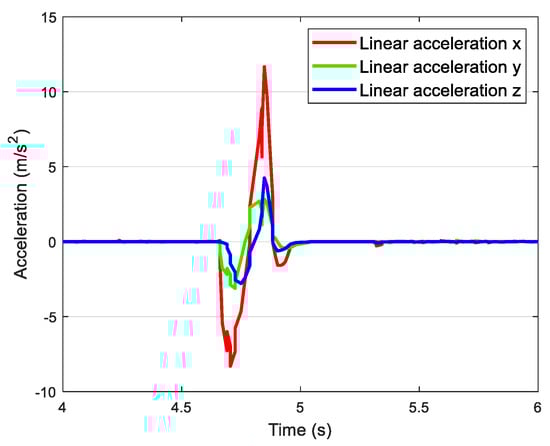
Figure 12.
Components of the unit linear acceleration vector.
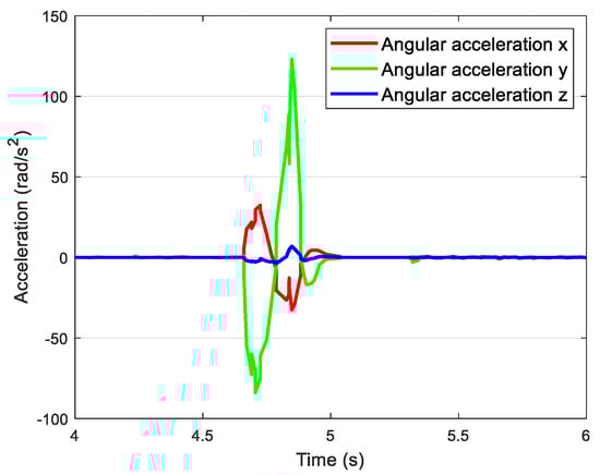
Figure 13.
Components of the angular acceleration vector.
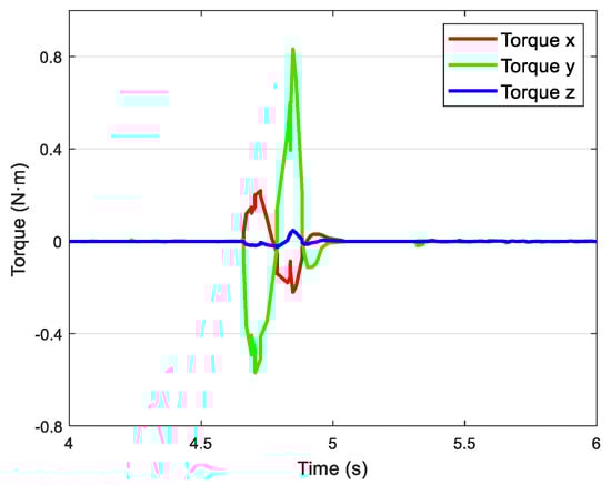
Figure 14.
Components of the output torque vector.
It can be seen from Figure 11 that the electromagnetic torque will quickly drive the rotor to reach the forward maximum velocity which is in the direction of the negative OX axis, then the rotor decelerates to zero in the influence of friction. As shown in Figure 12, the linear acceleration component of the rotor increases to the maximum positive value first driven by the electromagnetic force, and then decreases to zero due to the friction. This process corresponds to the stage that the velocity increases from zero to the maximum. In the influence of the friction, the linear acceleration component reaches the inverse maximum value and finally becomes zero. This process corresponds to the stage that the velocity increases from the maximum value to zero. Figure 13 shows that the change of the component of the angular acceleration vector on the OY axis is consistent with the component of the linear acceleration vector on the OX axis in Figure 12. As shown in Figure 14, the output torque increases rapidly from zero to the maximum value and then it gradually decreases to zero under the influence of the friction. In this stage, the rotor speed increases continuously under the influence of the output torque. When the electromagnetic force is less than the friction force, the rotor will slow down to the final stillness.
3.4. Comparison with Simulated Results
In order to compare with the simulated torque by the FEM, we take the output torque vector at the moment that the torque component on the OX axis reaches the maximum value at the first time as an example. This is the vector corresponding to the output torque at the starting time of the rotor. The torque components on the OX, OY and OZ axis of the coordinate system OXYZ at the moment are represented by , and , respectively. Thus, the output torque vector and its amplitude can be respectively written as:
Two motion cases are considered in the comparison with simulated results. In the first case, the initial rotor potion is stationary, and the total current of coils increased from 1.5 to 5.42 A. In the second case, the initial rotor position rotates around the OZ axis from 0 to 180 degrees and the total current of coils is fixed 4 A. In this case, each coil is energized by unit current. The current directions of No. 2 coil and No. 20 coil are positive as the same as shown in Figure 2, while the current directions of No. 8 coil and No. 20 coil are negative, which are opposite to that in Figure 2. The experimental results of the two cases are shown in Figure 15.
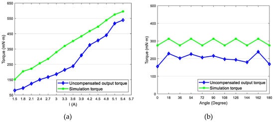
Figure 15.
Measured torques before compensation: (a) Measured torques at different currents; (b) Measured torques at different angles.
Taking the simulation torque as a reference, we define the measurement error as:
where denotes the simulation torque. The measurement errors of the two motion cases are shown in Table 2 and Table 3.
Table 2.
Measurement errors at different currents.
Table 3.
Measurement errors at different angles.
The output torque measured by the MEMS gyroscope sensor has a wide range of error from 9.48% to 53.54% in the coordinate system OXYZ.
3.5. Error Analysis and Compensation
The rotor of the PMSM is heavy, which causes great pressure on the contact surface of the support structure. Therefore, it inevitably brings error for measuring output torque during the start-up process of the rotor. When the rotor moves, the error caused by the friction will reduce the accuracy of torque measurement. This type of error can be estimated by repetitive experiments and the targeted error compensation can be conducted to improve the accuracy of the measurement.
In order to study the influence of friction torque on the measurement error of the output torque, the maximum static friction in the initial position of rotor is measured by a tension meter. Figure 16 shows the measurement of the maximum static friction. The distance from the top of the rotor output shaft to the center of the rotor is 0.1 m, that is, the force arm of the maximum static friction force is 0.1 m. The tension meter and the top of the output shaft are connected by a thin nylon wire. A spirit level is used to ensure that the tension is perpendicular to the output shaft. Then, the tension meter is slowly pulled along the negative direction of the OX axis and the data displayed in the tension meter are recorded at the moment of rotor startup. The measurement for static friction is repeatedly conducted by 20 times and the measured results are listed in Table 4.
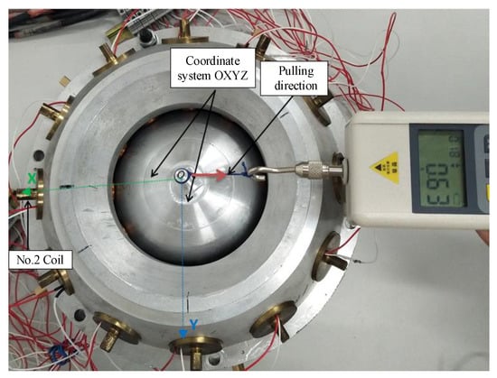
Figure 16.
Measurement of the maximum static friction.
Table 4.
Measurements of maximum static friction.
The average value of the static friction measured by the above 20 groups of experiments is used as the estimated maximum static friction for the compensation. The average is 69.7 mN·m. The output torques are compensated and are shown in Figure 17.
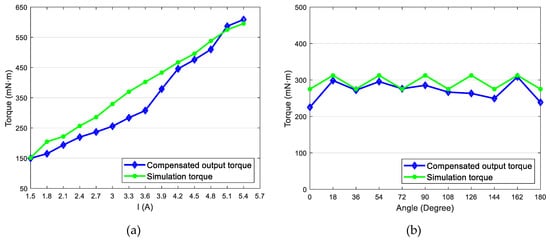
Figure 17.
Measured torques after compensation: (a) Measured torques at different currents; (b) Measured torques at different angles.
Table 5 and Table 6 show the measurement errors after the compensation, and it can be seen that the measurement errors decrease to 0.39–23.47%.
Table 5.
Measurement errors at different currents after compensation.
Table 6.
Measurement errors at different angles after compensation.
After the compensation of the maximum static friction, the remaining error can be analyzed in two ways. Firstly, since the initial position of the rotor is manually adjusted, the motor stator and rotor in the coordinate system OXYZ cannot be perfectly aligned, which will change the experimental motion conditions and affect the measurement of the output torque. Secondly, only the maximum static friction is considered in this paper for compensation because of the limitation of the experimental method. In fact, other complex friction which is not estimated will affect the effectiveness of the compensation.
4. Conclusions
This paper presents a torque measurement method for a permanent magnet spherical motor. The MEMS gyroscope sensor is used to obtain the dynamic information of the rotor at the starting moment. Based on the angular acceleration and the moment of inertia, the output torque of the rotor is calculated. The experiments are conducted to measure the output torque by using the MEMS gyroscope sensor and the measured results are compared to the simulated results by FEM. The maximum static friction is estimated by experiments and is utilized to compensate the measured results. The comparison results show the significant reduction in the measurement errors after compensation. Although the proposed method to measure the output torque is carried out under no-load conditions, it is theoretically applicable to load conditions.
Author Contributions
G.L. conceived and designed the analysis; Y.L., Y.W., and R.T. designed experiments; Y.W., R.T. and H.L. carried out experiments; G.L., Y.L., Y.W. and R.T. analyzed experimental results; R.T. wrote the original manuscript; Y.W., Y.L., and H.L. edited and improved the manuscript. Q.W. is the project administration and provided financial support. All authors have read and agreed to the published version of the manuscript.
Funding
This work is supported by the key project of the China National Natural Science Foundation (51637001).
Conflicts of Interest
The authors declare there is no conflicts of interest regarding the publication of this paper.
References
- Lee, K.M.; Vachtsevanos, K.; Kwan, C. Development of a Spherical Stepper Wrist Motor. J. Intell. Robot. Syst. 1998, 1, 225–242. [Google Scholar]
- Lee, K.M.; Son, H.S. Torque Model for Design and Control of a Spherical Wheel Motor. In Proceedings of the IEEE/ASME International Conference on Advanced Intelligent Mechatronics, Monterey, CA, USA, 24–28 July 2005. [Google Scholar]
- Xia, Y.; Li, G.; Qian, Z.; Ye, Q.; Zhang, Z. Research on rotor magnet loss in fractional-slot concentrated-windings permanent magnet motor. In Proceedings of the IEEE 11th Conference on Industrial Electronics and Applications, Hefei, China, 5–7 June 2016. [Google Scholar]
- Wang, A.; Wang, C.; Hu, C.; Qian, Z.; Ju, L.; Liu, J. An EKF for PMSM sensorless control based on noise model identification using Ant Colony Algorithm. In Proceedings of the 2009 International Conference on Electrical Machines and Systems, Tokyo, Japan, 15–18 November 2009. [Google Scholar]
- Rossini, L.; Onillon, E.; Chételat, O.; Perriard, Y. Force and Torque Analytical Models of a Reaction Sphere Actuator Based on Spherical Harmonic Rotation and Decomposition. IEEE ASME Trans. Mechatron. 2013, 18, 1006–1018. [Google Scholar] [CrossRef]
- Rossini, L.; Chételat, O.; Onillon, E.; Perriard, Y. An open-loop control strategy of a reaction sphere for satellite attitude control. In Proceedings of the 2011 International Conference on Electrical Machines and Systems, Beijing, China, 20–23 August 2011. [Google Scholar]
- Yan, L.; Chen, I.M.; Yang, G.; Lee, K. Analytical and Experimental Investigation on the Magnetic Field and Torque of a Permanent Magnet Spherical Actuator. IEEE-ASME Trans. Mechatron. 2006, 11, 409–419. [Google Scholar]
- Yan, L.; Chen, I.M.; Yang, G.; Lee, K. Design and Analysis of a Permanent Magnet Spherical Actuator. IEEE ASME Trans. Mechatron. 2008, 13, 239–248. [Google Scholar] [CrossRef]
- Kumagai, M.; Ochiai, T. Development of a Robot Balancing on a Ball. In Proceedings of the 2008 International Conference on Control, Automation and Systems, Seoul, Korea, 14–17 October 2008. [Google Scholar]
- Kumagai, M. Torque Evaluation Method of Spherical Motors Using Six-Axis Force/Torque Sensor. In Proceedings of the 2016 IEEE International Conference on Robotics and Automation, Stockholm, Sweden, 16–21 May 2016. [Google Scholar]
- Kasashima, N.; Ashida, K.; Yano, T.; Gofuku, A.; Shibata, M. Torque Control Method of an Electromagnetic Spherical Motor Using Torque Map. IEEE ASME Trans. Mechatron. 2016, 21, 2050–2060. [Google Scholar] [CrossRef]
- Qian, Z.; Wang, Q.; Ju, L.; Wang, A.; Liu, J. Torque Modeling and Control Algorithm of a Permanent Magnetic Spherical Motor. In Proceedings of the 2009 International Conference on Electrical Machines and Systems, Tokyo, Japan, 15–18 November 2009. [Google Scholar]
- Wang, W.; Wang, J.; Jewell, G.W.; Howe, D. Design and Control of a Novel Spherical Permanent Magnet Actuator with Three Degrees of Freedom. IEEE ASME Trans. Mechatron. 2003, 8, 457–468. [Google Scholar] [CrossRef]
- Lu, Y.; Hu, C.G.; Wang, Q.J.; Hong, Y.; Shen, W.X.; Zhou, C.Q. A New Rotor Position Measurement Method for Permanent Magnet Spherical Motors. Appl. Sci. 2018, 8, 2415. [Google Scholar] [CrossRef]
- Li, B.; Li, G.D.; Li, H.F. Magnetic Field Analysis of 3-DOF Permanent Magnetic Spherical Motor Using Magnetic Equivalent Circuit Method. IEEE Trans. Magn. 2011, 47, 2127–2133. [Google Scholar] [CrossRef]
- Changliang, X.; Peng, S.; Hongfeng, L.; Bin, L.; Tingna, S. Research on Torque Calculation Method of Permanent-Magnet Spherical Motor Based on the Finite-Element Method. IEEE Trans. Magn. 2009, 45, 2015–2022. [Google Scholar] [CrossRef]
- Liu, J.M.; Deng, H.Y.; Chen, W.H.; Bai, S.P. Robust dynamic decoupling control for permanent magnet spherical actuators based on extended state observer. IET Control Theory A 2017, 11, 619–631. [Google Scholar] [CrossRef]
- Wen, Y.; Li, G.; Wang, Q.; Guo, X. Robust Adaptive Sliding-Mode Control for Permanent Magnet Spherical Actuator with Uncertainty Using Dynamic Surface Approach. J. Electr. Eng. Technol. 2019, 14, 2341–2353. [Google Scholar] [CrossRef]
- Rong, Y.; Wang, Q.; Lu, S.; Li, G.; Lu, Y.; Xu, J. Improving attitude detection performance for spherical motors using a MEMS inertial measurement sensor. IET Electr. Power Appl. 2019, 13, 198–205. [Google Scholar] [CrossRef]


© 2020 by the authors. Licensee MDPI, Basel, Switzerland. This article is an open access article distributed under the terms and conditions of the Creative Commons Attribution (CC BY) license (http://creativecommons.org/licenses/by/4.0/).