Practical Control of a Cold Milling Machine using an Adaptive PID Controller

Featured Application

Coal Mining.

Abstract

This paper presents a supervised Hebb learning single neuron adaptive proportional-integral-derivative (PID) controller for the power control of a cold milling machine. The proposed controller aims to overcome the deficiency of the current power control algorithm, and to achieve as high an output power as possible for the cold milling machine. The control process and system model are established and presented to provide the insight and guidance to the controller design and analysis. The adaptive PID controller is developed using a supervised Hebb learning single neuron method with detailed algorithm and structure analysis. The field test is performed to validate the proposed single neuron adaptive PID control for the power control. In the test, the 8 cm-depth milling is conducted on a cement concrete pavement in which the cement is not well-distributed. The test results show that when the machine speed is adjusted by the machine itself or manually without the adaptive power control system, the machine is often overloaded or underloaded, and the average work speed is 2.4m/min. However, when the adaptive control system is implemented on the machine, it works very close to its rated work condition during its work process. With the developed controller, the machine work speed is adjusted in time to the load variation and uncertain dynamics. The average machine work speed can reach up to 2.766 m/min, which is 15.25% higher than the wok speed of the machine without an adaptive power control system.

1. Introduction

A cold milling machine is an off-highway vehicle which is widely used for the controlled surface removal of existing pavement to the desired depth in highway maintenance and reconstruction [1]. The amount of removal material can also be controlled to meet project specific requirements. The resulting textured pavement can be used immediately as a driving surface.

The structure and the working process of a cold milling machine are illustrated in Figure 1 and Figure 2. The machine is equipped with a cutting drum to mill the pavement surface to the specified grade and cross-slope. The cutting drum is equipped with picks, and is driven by the engine to whirl and mill the pavement as the machine moves. Milling removes material in a range varying anywhere from just enough thickness to level and smooth the surface to a full depth removal. Recycling of the road surface is one of the main reasons for milling a road surface. Milling is widely used for pavement recycling today, where the pavement is removed and ground up to be used as the aggregate in new pavement. Milling can also remove distresses from the surface, providing a better driving experience and longer roadway life. The cold milling machine is also a great tool for performing utility maintenance cuts, and ripping out roadways to repair foundations.

Due to variations of the thickness and material property to be milled at different construction sites, the load of the cold milling machine changes at random. This situation often causes the machine to being overloaded or underloaded, which leads to a low productivity of the machine. The reasons include: (1) When the machine is overloaded significantly, the engine speed is under large fluctuation. The speed of the cut rotator is changed with the engine speed. If the engine speed is down, the cut rotator cannot transmit all of the milled materials into the conveyor in time. However, the milled materials should be collected and put into the conveyor immediately after they are milled. As a result, lots of milled materials are piled up in the milling chamber and the power consumption on mixing milled materials increases. This consumption should be prevented to improve productivity. (2) When the engine speed fluctuates due to overloaded or underloaded conditions, its dynamic performance and fuel efficiency will decrease, and the average output power of the engine comes down. (3) When the machine is overloaded, the slip rate of the drive wheel will increase, which leads to the decrease of the work speed and a short life of the wheel.

It is very difficult to make full use of the engine power and to make the cold milling machine work in ideal conditions only by the operator’s experience and manual operation. The reason is that the load of a cold milling machine is dynamic and uncertain during its work process. Furthermore, the dynamics of the cold milling machine are nonlinear and uncertain, and therefore it is desirable to develop a proper power control system that is capable of automatically adjusting the machine so that it works at its rated power or in a highly efficient state. Guo and Duan [2] and Gu et al. [3] designed novel cutters of the cold milling machines to reduce the power consumption. Wang et al. [4] and Long [5] studied the theoretical methods of the power control for a cold milling machine, but specific power control algorithms were not proposed for the machine power control. Chen et al. [6] and Yuan [7] mainly conducted the hardware design of the power control system for a cold milling machine. Ma et al. [8,9] investigated the vehicle dynamics to realize the power control of a cold milling machine, but only numerical simulations were used to validate the proportional-integral-derivative (PID) controller and the PID parameters were fixed. A traditional PID controller with the fixed-control gains cannot achieve the optimal control performance and is not adaptive to environment variations for the cold milling machine power control featured with a nonlinear and uncertain system [10,11]. There are several alternative control methods, such as neural network control [12,13,14,15], fuzzy control [16,17,18], robust control [19,20,21,22], and adaptive control [17,18,19,20]. The neural network control has strong self-study ability to control a nonlinear system, but it needs lots of computation. It is not feasible as the cold milling machine is equipped with a 16 bit single chip microcomputer, which has a very limited computation capability. The performance of fuzzy controllers depends on the fuzzy rules which are difficult, if not possible, to be identified completely from our work experience at present. Therefore the fuzzy control is not selected to be an appropriate alternative for cold mining machines. Most of the robust control needs a reference model or sensitive coefficients [19,20,21,22]. However, it is not possible for us to establish a reliable reference model and determine sensitivity coefficients that are needed in the controller design of the cold milling machine. Obviously, the robust control is not the option in the power control of a cold milling machine. Two typical adaptive control methods are STC (self-tuning control) and MRAC (model reference adaptive control). The MRAC needs a reference model which is not available for cold mining machines [23,24]. The STC needs online identification and synthetic decision [25,26]. There are little such synthetic decision algorithms and strategies for a cold milling machine at present. Therefore, the typical adaptive control is ruled out in this work.

The single neuron control is a proper option as it possesses the strong ability of self-studying and self-adapting. The single neuron is used to adjust the control gains of the PID controller online, and hence it can overcome the shortage of the fixed control gains in traditional PID controllers. This single neuron PID not only has the characteristics of the neural network control but also has the characteristics of the PID control. Therefore, the single neuron PID can be implemented more easily in engineering application than the neural network control, the fuzzy control, the robust control and adaptive control. Furthermore, the strong ability of self-studying and self-adapting of the single neuron PID control can improve the performance and robustness of the adaptive power control.

In order to address the practical control challenge for cold mining machines, this paper proposes a supervised Hebb learning single neuron PID method. The contributions of this work include: (1) this work attempts to develop and implement the proposed controller on a real machine with field testing; (2) in this work the control gain is tuned by a supervised Hebb learning algorithm, so the proposed controller can adapt to the environment variations; (3) the supervised Hebb learning based PID controller does not need any Sign functions to adjust the PID gains; therefore, the control performance is much more steady and accurate than that of the Sign function-based PID controllers. Field testing result demonstrates the performance of the proposed method.

This paper is organized as follows. In Section 2 the control process and the system model of a cold milling machine are established to provide the guidance to control design and analysis. Section 3 presents the integration of the single neuron adaptive power PID controller to the power control for a cold milling machine. The control algorithm implementation is detailed in Section 4. Section 5 is dedicated to the analysis and discussion of the field test results. The conclusions are given in the last section.

2. Control Model

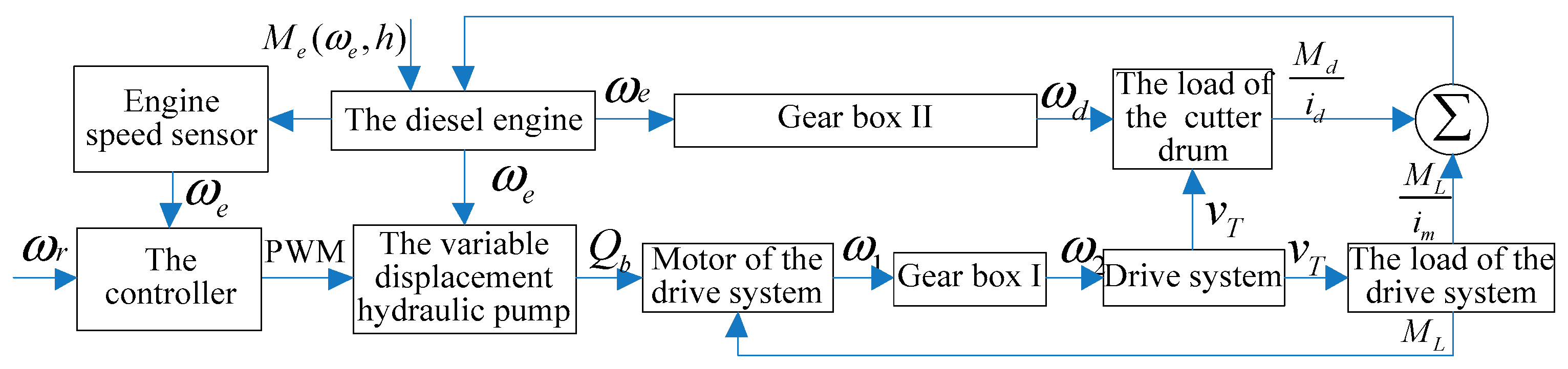
2.1. Control System Overview

The power control process is illustrated in Figure 3. As shown in Figure 3, the engine has two inputs: one from ECU (electronic control unit) and the other one from the load. The input from ECU is fixed and should not be changed during the machine work process to meet the variable heavy loads. This work focuses on how to control the duty cycle of the PWM so that the load of the machine acting on the engine regulates the engine speed to be as constant as possible and achieve the output power to be as high as possible.

The displacement of the variable displacement hydraulic pump controls the flux $Q_b$ of the variable pump. The flux $Q_b$ determines the hydraulic motor rotary speed ${\omega }_1$. The drive wheel is connected with the motor through gearbox I whose ratio is fixed, i.e., the drive wheel rotary speed ${\omega }_2$ is proportional to ${\omega }_1$ and the wheel theoretical moving speed $v_T$. As detailed in Equation (15) and (20), the variation of $v_T$ leads to the load change of the cold milling machine. It is clear that the power consumption of the cold milling machine is adjusted through this control process when the load of the machine is changed. On the other hand, the cutting drum is connected with the engine through gear box II whose ratio is about 10. In Figure 3, $i_d$ is the transmission ratio from the engine to the milling drum, $i_m$ denotes the transmission ratio from the engine to the hydraulic motor, and $h$ refers to the position of the throttle. This process can be described using the following system model.

2.2. System Model

2.2.1. Engine Model

According to [26], the dynamic model of the engine can be given as

$$J{\stackrel{•}{\omega }}_e=M_e({\omega }_e,h)-M_I^c(t)$$

(1)

where J is the moment of inertia of the engine, M_e is the input torque to the engine, and $M_I^c$ is the resisting moment torque acted on the bent axle of the engine. $M_e\left({\omega }_e,h\right)$ is related with the engine speed ${\omega }_e$ and a nonlinear throttle function $h$. Therefore, the diesel engine is a nonlinear system.

Taking Taylor expansion and Laplace transform, linearization through the Taylor series concerns the development at a fixed working point. Therefore, after linearization, an increment of a variable should be used instead of a variable. The model of the system linearizes around the rated working parameter. When variables are fluctuated slightly around in the local region of working points, the result of numerical calculation is more accurate, which is proved in reference [26]. Equation (1) is rewritten as:

$$(M_e^{\prime }({\omega }_{e0},h)-Js){\omega }_e(s)=M_I^c(s)$$

(2)

2.2.2. Model of Drive System

The flux function of the variable hydraulic displacement pump can be described as,

$$Q_b=K_b{i}_e{\omega }_e{\varphi }_b-C_{ib}(P-P_r)-C_{eb}P$$

(3)

where $Q_b$ is the flux of the hydraulic pump, $K_b$ is the displacement gradient of the hydraulic pump, $i_e$ is the transmission ratio of the gearbox between the engine and the pump, $C_{ib}$ is the internal leakage coefficient of the pump, $P$ is the work pressure of the pump, $P_r$ is the backpressure of the hydraulic system, $C_{eb}$ is the external leakage coefficient of the pump, and ${\varphi }_b$ is the angle of the sliding shoes in the pump. Here, ${\varphi }_b$ is proportional to the control voltage $u$ of the hydraulic pump [27]:

$${\varphi }_b=k_{\varphi }u$$

(4)

where $k_{\varphi }$ is a constant.

Substituting Equation (4) into Equation (3), and taking the result linearization and Laplace transform, it yields

$$Q_b(s)=K_b{i}_e{k}_{\varphi }{\omega }_{e0}u(s)+K_b{i}_e{k}_{\varphi }{u}_0{\omega }_e(s)-C_{b}P(s)$$

(5)

where $C_b=C_{ib}+C_{eb}$ is the total leakage coefficient of the hydraulic pump, ${\omega }_{e0}$ and $u_0$ are the initial values. $P_r$ is the back pressure of the hydraulic system which is a constant in Equation (3), when we take Laplace transform of Equation (3), $P_r$ is zero.

The flux continuity function of the motor is given by [27]:

$$Q_b-C_{im}(P-P_r)-C_{em}P=D_m\stackrel{•}{{\theta }_m}+\frac{V_0}{{\beta }_e}\stackrel{•}{P}$$

(6)

Taking Laplace transform, Equation (6) is rewritten as

$$Q_b(s)-C_{m}P(s)=D_{m}s{\theta }_m(s)+\frac{V_0}{{\beta }_e}sP(s)$$

(7)

where $C_{im}$ is the internal leakage coefficient of the hydraulic motor; $C_{em}$ is the external leakage coefficient of the motor, $D_m$ is the displacement of the hydraulic motor, ${\theta }_m$ is the rotation angle of the motor axle, $V_0$ is the total volume of the high pressure chamber of the pump, motor and hydraulic pipe, ${\beta }_e$ is the modulus elastic of the hydraulic oil volume, and $C_m$ is the total leakage coefficient of the hydraulic motor.

The torque balance function of the hydraulic motor can be derived as

$$D_m(P-P_r)=J_m\stackrel{••}{{\theta }_m}+B_m\stackrel{•}{{\theta }_m}+M_L$$

(8)

where $M_L$ is the load of the hydraulic motor.

The transform function of Equation (9) is given as

$$D_{m}P(s)=(J_m{s}^2+B_{m}s){\theta }_m(s)+M_L(s)$$

(9)

The relationship between the work speed and the angular velocity of the hydraulic motor can be expressed as

$$v_T(s)=\frac{2\pi R_{g}s{\theta }_m(s)}{i_g}$$

(10)

Where $i_g$ is the transmission ratio from the hydraulic motor to the drive wheel.

Combining Equations (5) (7) (9) and (10), the model of the pump control motor system can be established as

$$K_{v_T}{v}_T(s)+K_{T_L}{M}_L(s)=K_b{i}_e{k}_{\varphi }{\omega }_{e0}u(s)+K_b{i}_e{k}_{\varphi }{u}_0{\omega }_e(s)$$

(11)

where

$$\begin{gathered} K_{T_L}=\frac{C_t}{D_m}\left(1+\frac{V_0}{C_t{\beta }_e}s\right),C_t=C_b+C_m, \\ {K}_{v_T}=\frac{D_m}{2\pi R_g}\left[\frac{J_m{V}_0}{D_m^2{\beta }_e}{s}^2+\left(\frac{B_m{V}_0}{D_m^2{\beta }_e}+\frac{C_t{J}_m}{D_m^2}+J_m\right)s+B_m\left(1+\frac{C_t}{D_m^2}\right)\right] \end{gathered}$$

The torque balance function of the milling drum is expressed as

$$J_d{\stackrel{•}{\omega }}_d+C_d{\omega }_d+M_d=M_{de}$$

(12)

where $M_{de}$ is the part of engine output torque transmitted from Gearbox II in Figure 3, $J_d$ the moment of inertia of the milling rotor, $C_d$ the rotational damp of the milling rotor. ${\omega }_d$ the rotary speed of the cutting drum, $M_d$ the resistance torque of the milling rotor, and $M_{de}$ the input torque of the milling rotor.

In a cold milling machine $J_d{\stackrel{•}{\omega }}_d+C_d{\omega }_d\le M_d$, Equation (12) can be described as

$$M_d=M_{de}$$

(13)

The milling force of the milling equipment is given by

$$F_r=\frac{b{k}_{\mathrm{d}}B{\tau }_{\mathrm{s}}{a}_{\mathrm{e}}{a}_{\mathrm{p}}{f}_Z(v_T^2+v_T{R}_{\mathrm{d}}^{}{\omega }_{\mathrm{d}}^{})}{Z_{\mathrm{d}}a{R}_{\mathrm{d}}^2{\omega }_{\mathrm{d}}^2}$$

(14)

where ${\gamma }_0$ is the realistic milling angle of the cutting pick, $b=\left(\frac{\cos {\gamma }_0}{\sin \left(\frac{\pi }{4}-\frac{\beta }{2}+\frac{{\gamma }_0}{2}\right)}+\frac{\sin \beta }{\cos \left(\frac{\pi }{4}+\frac{\beta }{2}-\frac{{\gamma }_0}{2}\right)}\right)$, $\beta$ is the friction angle of the pick front surface, $Z$ is the cutting pick number on the cutting drum, $f_Z$ is the milling feed rate of each cutting pick on the cutting drum, ${\omega }_{\mathrm{d}}$ is the milling drum rotary speed, $a_{\mathrm{p}}$ is the milling depth, $a_{\mathrm{e}}$ is the milling thickness, $a=\left(\frac{\pi }{4}-\frac{\beta }{2}-\frac{{\gamma }_0}{2}\right)$, ${\tau }_{\mathrm{s}}$ is the splitting failure strength of the material to be milled which changes at random at a not well-distributed pavement, $B$ is the milling width, $R_{\mathrm{d}}$ is the radius of the cutting drum, and $k_{\mathrm{d}}$ is a constant.

The milling torque $M_d$ can be calculated by

$$M_d=\frac{b{k}_{\mathrm{d}}B{\tau }_{\mathrm{s}}{a}_{\mathrm{e}}{a}_{\mathrm{p}}{f}_Z(v_T^2+v_T{R}_{\mathrm{d}}^{}{\omega }_{\mathrm{d}}^{})}{Z_{\mathrm{d}}a{R}_{\mathrm{d}}^{}{\omega }_{\mathrm{d}}^2}$$

(15)

Taking linearization and Laplace transform, Equation (15) is simplified as

$$M_d(s)=k_{\omega d}{\omega }_d(s)+k_{{\tau }_{\mathrm{s}}}{\tau }_{\mathrm{s}}(s)+k_{v_T}{v}_T(s)$$

(16)

where

$$\begin{gathered} k_{{\tau }_{\mathrm{s}}}=\frac{b{k}_{\mathrm{d}}B{a}_{\mathrm{e}}{a}_{\mathrm{p}}{f}_{\mathrm{Z}}\left(v_{T0}^2+v_{T0}{R}_{\mathrm{d}}{\omega }_{d0}\right)}{Z_{\mathrm{d}}a{R}_{\mathrm{d}}{\omega }_{d0}^2}, \\ {k}_{\omega d}=\frac{b{k}_{\mathrm{d}}{\tau }_{\mathrm{s}0}{a}_{\mathrm{e}}{a}_{\mathrm{p}}{f}_{\mathrm{Z}}{v}_{T0}}{Z_{\mathrm{d}}a{\omega }_{d0}^2}-\frac{2b{k}_{\mathrm{d}}B{\tau }_{\mathrm{s}0}{a}_{\mathrm{e}}{a}_{\mathrm{p}}{f}_{\mathrm{Z}}\left(v_{T0}^2+v_{T0}{R}_{\mathrm{d}}{\omega }_{d0}\right)}{Z_{\mathrm{d}}a{R}_{\mathrm{d}}{\omega }_{d0}^3}, \\ {k}_{v_T}=\frac{b{k}_{\mathrm{d}}B{a}_{\mathrm{e}}{a}_{\mathrm{p}}{f}_Z\left(2v_{T0}+R_{\mathrm{d}}{\omega }_{d0}\right)}{Z_{\mathrm{d}}a{R}_{\mathrm{d}}{\omega }_{d0}^2} \end{gathered}$$

When the cold milling machine is running, it is driven by the driving wheel. The dynamics of the tractive system can be described as

$$m\stackrel{•}{v_T}+k{v}_T+F_f+F_{\mathrm{H}}=F_{\mathrm{K}}$$

(17)

where $m$ is the mass of the machine, $k$ the speed damp coefficient, $F_{\mathrm{H}}$ the level component force of the milling equipment, $F_f$ the wheel rolling resistance which is a constant, and $F_{\mathrm{K}}$ the tangent tractive force.

When the machine is working along a straight road slowly, the speed resistance can be ignored. Therefore, Equation (17) can be expressed as

$$m\stackrel{•}{v_T}+F_H=F_K-F_f$$

(18)

where $F_{\mathrm{K}}=\frac{i{M}_{\mathrm{L}}}{R_0}$, $R_0$ is the dynamics radius of the driving wheel, and $i$ the transmission ratio from the motor to the driving wheel.

Taking Laplace transform, Equation (18) is given as

$$ms{v}_T(s)+F_H(s)=\frac{i{M}_L(s)}{R_0}$$

(19)

The working resistance $F_H$ is given by [8]:

$$F_H=\frac{M_d}{k_{md}{R}_d}+k_{\mathrm{h}}B{a}_{\mathrm{e}}^2{v}_T$$

(20)

Based on Equations (15), (19) and (20), we can get the transform function of the ground drive system of the machine:

$$ms{v}_T(s)+k_{dr}{v}_T(s)=k_{i0}{M}_L(s)-k_{i1}{\omega }_d(s)-k_{i2}{\tau }_{\mathrm{s}}(s)$$

(21)

where

$$k_{i0}=\frac{i}{R_0},k_{i1}=\frac{k_{{\omega }_{\mathrm{d}}}}{k_{md}{R}_d},k_{i2}=\frac{k_{{\tau }_{\mathrm{s}}}}{k_{md}{R}_d},k_{dr}=\frac{\left(k_{v_{\mathrm{T}}}+k_{md}{R}_d{k}_{h}B{a}_e{}^2\right)}{k_{md}{R}_d}$$

The engine resisting moment torque can be expressed using the load of the hydraulic motor and the milling torque as:

$$M_I^c(s)=\frac{M_d(s)}{i_d}+\frac{M_L(s)}{i_m}$$

(22)

Based on Equations (2), (11), (16), (21) and (22), we can get the transform function of the main power consumption of the machine as

$$Js{\omega }_e(s)+K_{{\omega }_e}(s){\omega }_e(s)=K_{up}(s)u(s)-K_{{\tau }_{\mathrm{s}}}(s){\tau }_{\mathrm{s}}(s)-K_P(s)P(s)$$

(23)

where

$$\begin{gathered} K_P\left(s\right)=-\frac{2\pi k_{v_{\mathrm{T}}}{R}_g{i}_g}{i_d{D}_m}\left(C_t+\frac{V_0}{{\beta }_e}s\right), \\ {K}_{{\omega }_e}\left(s\right)=\frac{\left[K_b{i}_e{k}_{\varphi }{u}_0\left(ms+k_{dr}\right)+K_{v_{\mathrm{T}}}{k}_{i1}\right]}{i_m{i}_d\left[K_{T_{\mathrm{L}}}\left(ms+k_{dr}\right)+K_{T_L}{k}_{i0}\right]}+\frac{2\pi k_{v_{\mathrm{T}}}{R}_g{i}_g{K}_b{i}_e{k}_{\varphi }{u}_0}{i_d{D}_m}+\frac{k_{{\omega }_d}}{i_d^2}-M_e^{\prime }\left({\omega }_{e0},h\right), \\ {K}_{{\tau }_{\mathrm{s}}}=\frac{k_{v_T}{k}_{i2}}{i_m\left[K_{T_L}\left(ms+k_{dr}\right)+K_{T_L}{k}_{i0}\right]}+\frac{k_{{\tau }_{\mathrm{s}}}}{i_d}, \\ {K}_{up}\left(s\right)=-\frac{K_b{i}_e{k}_{\varphi }{\omega }_{e0}\left(ms+k_{dr}\right)}{i_m\left[K_{T_L}\left(ms+k_{dr}\right)+K_{T_L}{k}_{i0}\right]}-\frac{2\pi k_{v_T}{R}_g{i}_g{K}_b{i}_e{k}_{\varphi }{\omega }_{e0}}{i_d{D}_m} \end{gathered}$$

The engineering application shows that the fluctuation value of the hydraulic pressure $P$ is very small during the work process of the cold milling machine, and hence $P$ can be treated as a constant. As a result, Equation (24) can be described as

$$Js{\omega }_e(s)+K_{{\omega }_e}(s){\omega }_e(s)=K_{up}(s)u(s)-K_{{\tau }_{\mathrm{s}}}(s){\tau }_{\mathrm{s}}(s)$$

(24)

To describe this system model much more simply and clearly, the model of the main power consumption parts has been linearized. It is clear that the cold milling machine is a nonlinear system that can be demonstrated by nonlinear terms, the engine model in Equation (1), the pump model in Equation (3), and the work equipment in Equation (20). As is shown in Equation (24) that the cold milling machine is a time varying system and there is a random disturbance ${\tau }_{\mathrm{s}}$ during the machine work process. Equation (24) shows that the engine speed ${\omega }_e$ will change if the splitting failure strength ${\tau }_{\mathrm{s}}$ is changed. To control the engine speed, the controller output voltage $u$ needs to be regulated to control the work speed in time so that the engine speed can be kept as constant as possible.

Obviously, the raditional PID controller cannot make the system achieve desirable performance as the system is nonlinear, uncertain, and time-varying.

Therefore, a single neuron adaptive power control algorithm is chosen to design the power control system of the milling machine.

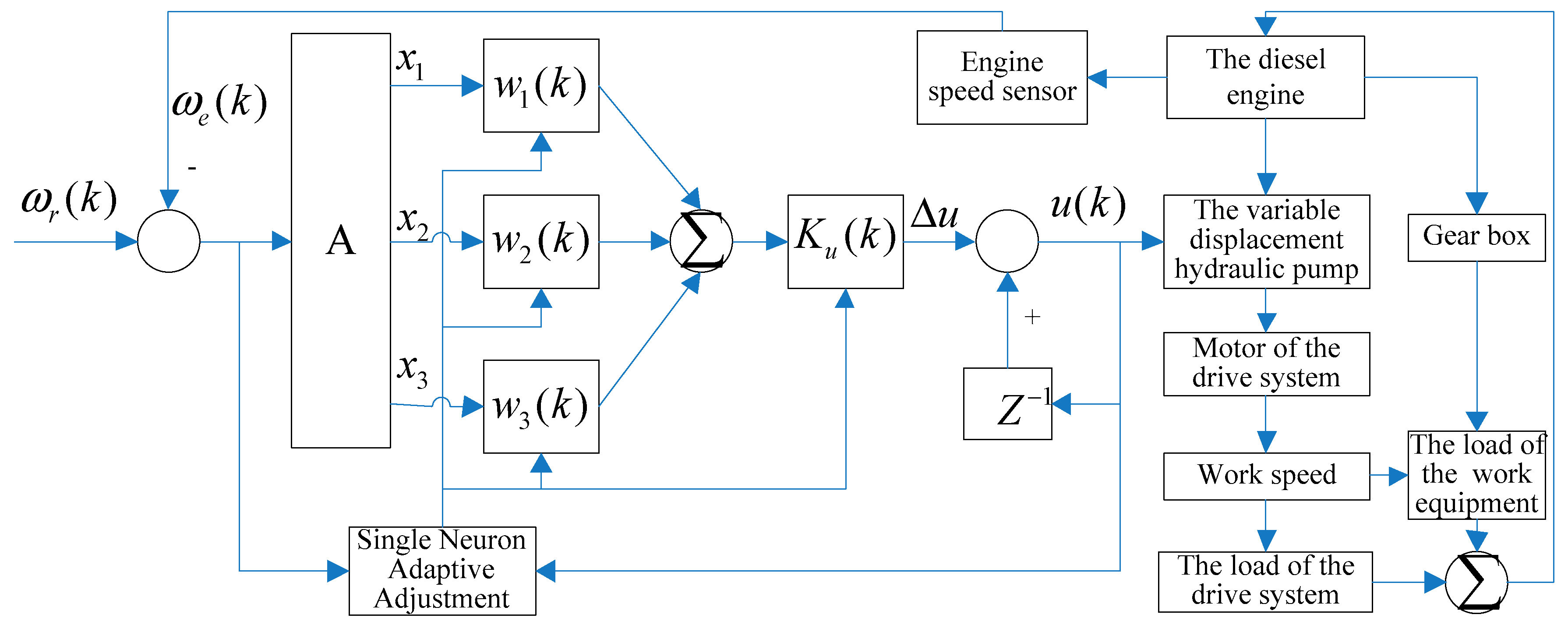
3. The Proposed Adaptive PID Controller

The structure of the single neuron adaptive power control system of a cold milling machine is similar to the fuzzy adaptive control system. In the single neuron adaptive power control system, the fuzzy adaptive control unit is replaced by the single neuron adaptive control unit. The weights of the PID controller are cumulated by the single neuron control algorithmic online continuously, which is different to the fuzzy control [28,29]. To implement the digital control, the system must be discretized.

The driver of a cold milling machine often places the throttle of the engine at its maximum position to meet the variation of the heavy load when the machine is working. The load of the machine can be adjusted by its work speed as the analysis in Section 2, if the throttle is fixed. The machine work speed can be adjusted by the displacement of the variable pump. The adjustment of the displacement is done through the single neuron adaptive power control system. Therefore, the output power of the engine is controlled by the control system. Based on the control mechanism of a traditional PID, the structure of the single neuron adaptive power PID controller designed for the cold milling machine is shown in Figure 4. The controller is used to improve the control responding speed and robustness performance to increase the productivity of the cold milling machine. In Figure 4, ${\omega }_e(k)$ is the engine speed, ${\omega }_r(k)$ denotes the engine reference speed, A is the converter, $u$ refers to the output of the control system, the output is to control the displacement of a pump, $x_1$, $x_2$, $x_3$ are the inputs of the PID controller, $K_u$ is the control gain which can be tuned with the control error, and ${\omega }_i(k)$ (i = 1, 2, 3) are the weights which are tuned by the single neuron adaptive adjustment.

According to the above structure, ${\omega }_e(k)$ and ${\omega }_r(k)$ are the reference input (desired speed) and actual output (measured engine speed) of the system, respectively, and the error satisfies $e(k)={\omega }_r(k)-{\omega }_e(k)$. It is assumed that ${\omega }_e(k)$ is measurable. In the view of the single neuron adaptive-PID controller, the input is $e(k)$ and the output is the incremental duty cycle of PWM $\mathsf{\Delta }u(k)$ driving the pump motor. Similar to a normal PID controller [30], the variables, $x_1$, $x_2$, $x_3$ satisfy the following relations respectively:

$$\begin{array}{c}{x}_1(k)={\omega }_r(k)-{\omega }_e(k)=e(k)\\ x_2(k)=e(k)-e(k-1)\\ x_3(k)=e(k)-2e(k-1)+e(k-2)\end{array}\}$$

(25)

where $e(k)$ is the deviated value.

In the algorithm of the single neuron PID control, the critical issue is to choose the learning rate. If $K_u$ in Equation (26) is a constant, we must set the learning rate ${\eta }_i$ for PID respectively and carefully, which is very tedious in the engineering application. To simplify the control parameter setting in the engineering application, the online correction of nonlinear transformation about parameter $K_u$ is used in this control system and can be given by,

$$K_u(k)=K_{u0}+\frac{\lambda {[{\omega }_r(k)-\omega (k)]}^3}{{\omega }^2{}_r(k)}$$

(26)

where $K_{u0}$ is a constant, $\lambda =0{.1\mathrm{K}}_{u0}$ in this control system. $K_u$ has a great impact on the system stability and rapidity. When the value of $K_u$ is small, the control system is comparatively of slow response and the overshoot of system could decrease. When the value of $K_u$ is large, the control system is of fast response, but the overshoot of the system increases with the long adjustment time. At the beginning of dynamic response, deviation $e\left(k\right)$ is large, the value of $K_u$ should be large in order to accelerate response. The deviation $e\left(k\right)$ approaches to zero in steady state, the value of $K_u$ should be decreases gradually until it reaches the steady value to ensure that the system is stable and small overshoot. Weights ${\omega }_i\left(k\right)$ changes adaptively with the value of deviation $e\left(k\right)$, and ultimately the process value will track the set value. Therefore it is necessary to select the online correction of nonlinear transformation in the Equation (26). From Equation (26), one can see that $K_u$ is changed with the error of the engine speed. If the error is small, $K_u=K_{u0}$. If the error is large, $K_u$ increases to be very large which leads to increasing the convergence speed of the control system. The advantage of this method is that we only need to select a proper $K_{u0}$, and there is no need to set the learning rate repeatedly. The online correction of $K_u$ is conduced to reduce the influence of the learning rate in this method.

In the single neuron PID control [31,32], the control law can be expressed by

$$\mathsf{\Delta }u(k)=K_u{\displaystyle \sum _{i=1}^3\frac{w_i(k)x_i(k)}{{\displaystyle \sum _{i=1}^3\left|w_i(k)\right|}}}$$

(27)

The single neuron adaptive PID controller implements the function of the adaptive- and self-learning by adjusting weight coefficients, which can form different control algorithms using different learning rules. Unsupervised learning functions as self-organized learning, i.e., the network learning is a completely self-learning process. The fundamental principle of Hebb learning is that if two neurons are activated at the same time, then the increase of their connect intensity is directly proportional to the product of their stimulation. Introducing a teacher signal into the Hebb learning algorithm leads to changing the output to the difference between ideal output and actual output. Basically, the supervised Hebb learning algorithm combines the unsupervised Hebb learning algorithm with the supervised Delta learning algorithm in [33]. In this work, the supervised Hebb learning algorithm is used to design the control law.

In the supervised Hebb learning algorithm, the weight value adjustment function is expressed as [34,35]

$$w_i(k+1)=w_i(k)+{\eta }_i{p}_i(k)$$

(28)

$$p_i(k)=K_u(k)z(k)u(k)x_i(k)$$

(29)

where $p_i\left(k\right)$ is the recursive signal and hushes gradually during the process, ${\eta }_i\left(i=P,I,D\right)$ is the learning rate, and $z\left(k\right)=e\left(k\right)$ is output error.

Substituting Equation (29) into Equation (28) one can get the weight increment $\mathsf{\Delta }{w}_i(k)$,

$$\mathsf{\Delta }{w}_i(k)=w_i(k+1)-w_i(k)={\eta }_i{K}_u(k)e(k)u(k)x_i(k)$$

(30)

To ensure the astringency and robustness of Equation (30) and $u\left(k\right)$ in the learning algorithm of single neuron adaptive PID controller, learning algorithms should be disposed canonically as

$$\begin{array}{l}u(k)=u(k-1)+K_u{\displaystyle \sum _{i=1}^3\frac{w_i(k)x_i(k)}{{\displaystyle \sum _{i=1}^3\left|w_i(k)\right|}}}\\ w_1(k+1)=w_1(k)+{\eta }_I{K}_{u}e(k)u(k)x_1(k)\\ w_2(k+1)=w_2(k)+{\eta }_P{K}_{u}e(k)u(k)x_2(k)\\ w_3(k+1)=w_3(k)+{\eta }_D{K}_{u}e(k)u(k)x_3(k)\end{array}\}$$

(31)

The weights of the neuron are trained using the simulation method until getting satisfied regulating results. Then the neuron adjuster operating mode is set by manual to non-automatic correction weights mode. According to simulation results of the system and practical trials, the system is convergent. For a cold milling machine, which is a very complicated system, the parameters calculated with the training data significantly deviate from the actual condition. The initial parameters in the system are determined through the trial and error method in the field tests.

4. Simulation Redults

4.1. Parameters’ Confirmation in the Model of the Cold Milling Machine

Based on the design parameter of actual cold milling machine and references [8,36,37,38], the parameters confirmation in the model is in

Table 1. Parameters confirmation in the model.

Variable	Value	Variable	Value
ie	1	h	100%
J(kg·m2)	0.459	Rg (m)	0.34
Dm(m3/rad)	4.16 × 10−5	Jd(kg·m2)	0.536
βe(MPa)	1.25 × 103	V0(m)	1.27 × 10−5
τs (MPa)	2.55	Cm(m−5·(N·s)−1)	1.4 × 10−12
nmax (rev·min−1)	2200	Zd	112
nH (rev·min−1)	2000	nMmax (rev·min−1)	1400
P H (kW)	196	Mmax (Nm)	1140
R0 (m)	0.34	M H (Nm)	937
B (m)	1.3	F f (N)	2800
Rd (m)	0.46	k	0.607
KP (m3·rad−1)	1.59 × 10−4	kd	0.9
β(rad)	0.174	kmd	2
ae(m)	0.08	γ0(rad)	0.209
ap(m)	0.08	im	230
id	12.5	ηP	2.6
m(kg)	20,000	ηD	0.05
ηI	1.25	w1	0.3
Ku0	0.065	w3	0.01
w2	0.13

.

Where $n_{\max }$ is the engine maximum speed, $n_{M\max }$ is the engine speed when the torque is the most maximum, $M_{\max }$ is the maximum torque, $n_H$ is the rated speed, $M_H$ is the rated torque.

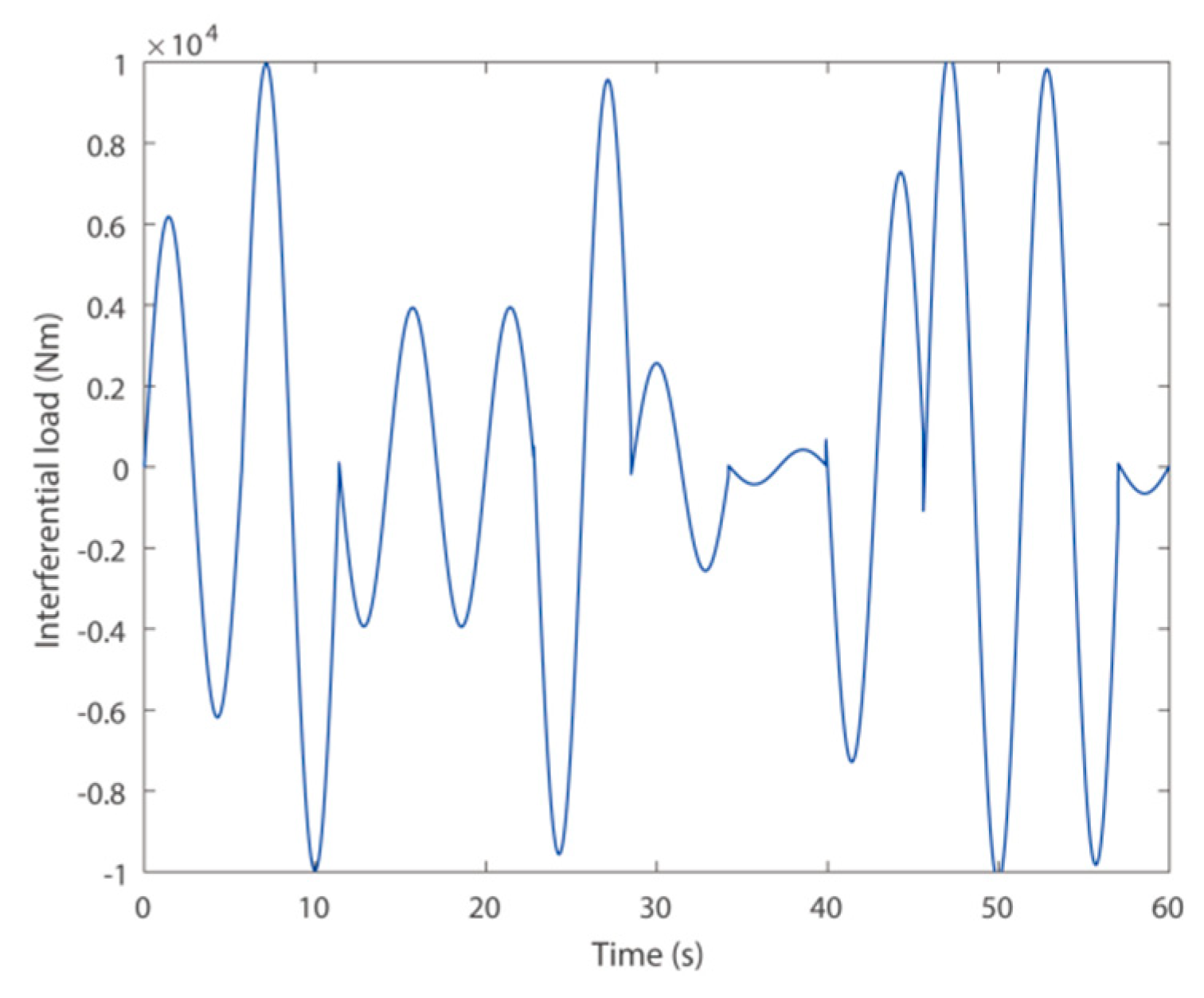
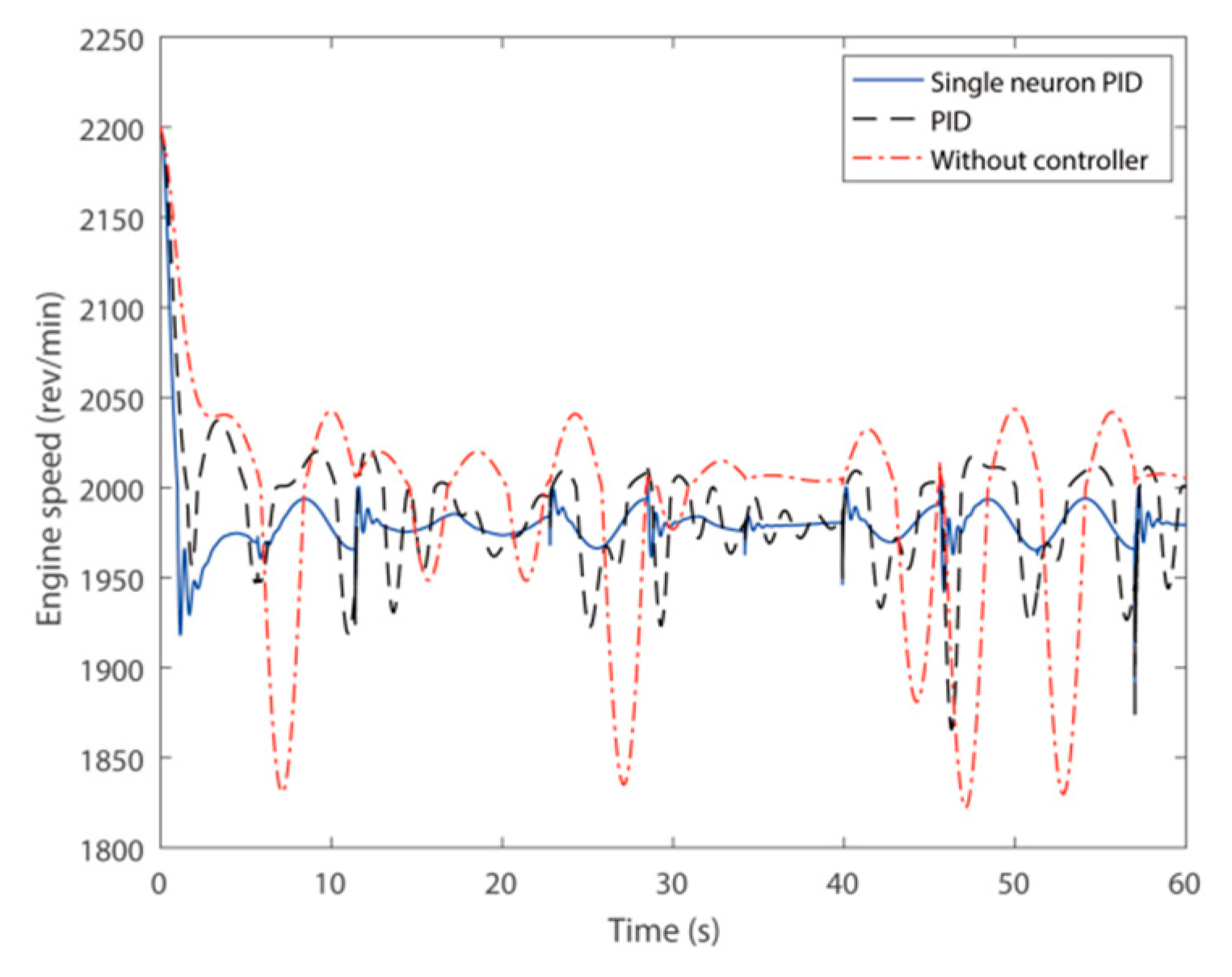
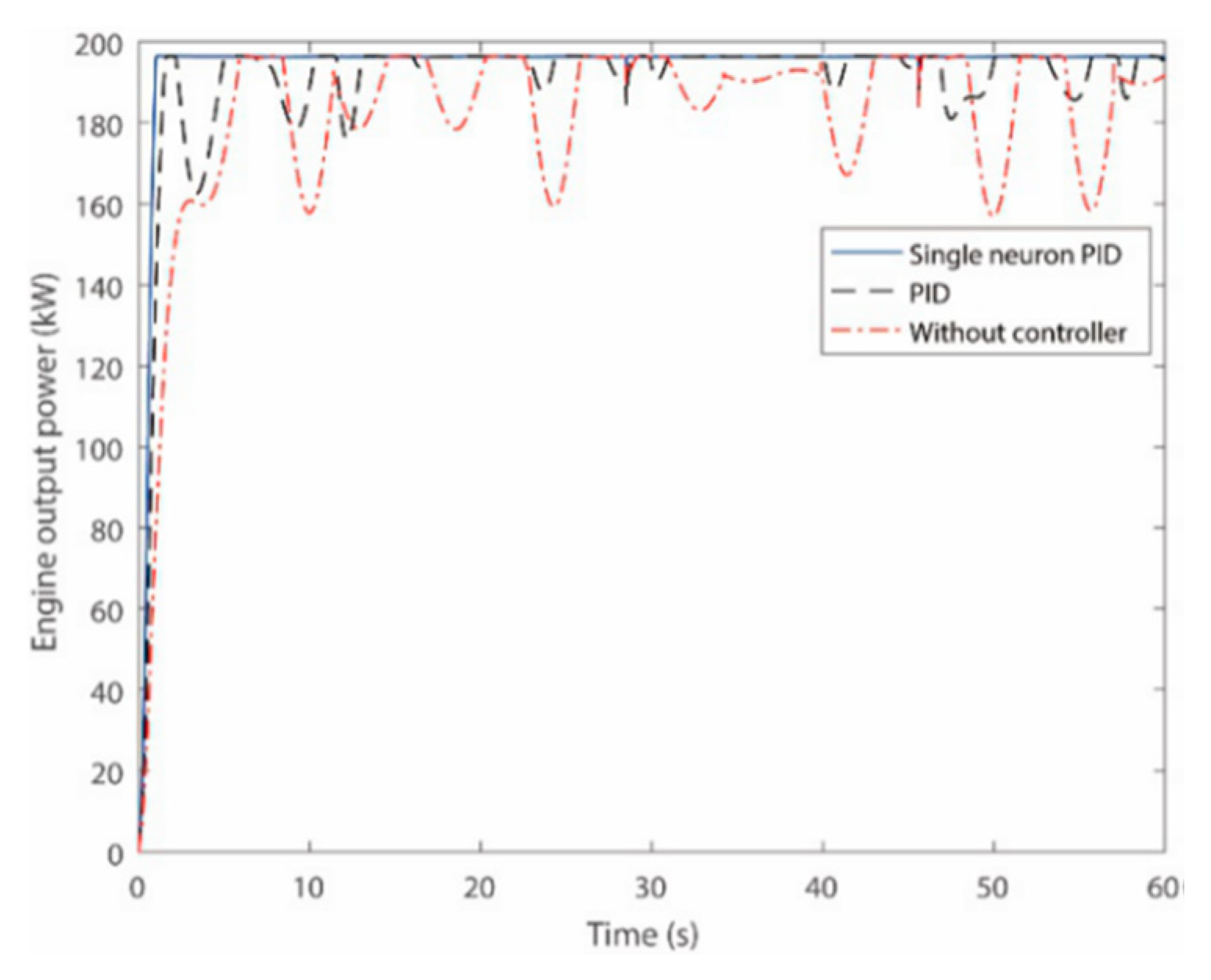
4.2. Simulation Results

It takes 60 s to finish the simulation. The simulations results in Figure 5, Figure 6, Figure 7 and Figure 8 show the machine with or without the power control system equipped. The load variation is simulated by an interference load which is shown in Figure 5. In order to observe the laws which are changed with the machine working load expediently, the sine wave with amplitude changing at random is selected as the interferential load. The engine reference speed of the control system is 1980 rev/min. The single neuron PID, the traditional PID and the manual operation are simulated with the model to help us selected a suitable control algorithm.

Figure 6 and Figure 8 show that when a single neuron PID power controller is equipped on the machine, the average work speed is 3.43 m/min and the engine rotary variation is 68 rev/min during its normal work process. Figure 7 shows that the engine output power amplitude variation is 9 kW and the average output power is 194.4 kW as well as the usage ratio of engine rated power is 99.2%, it works very close to its rated work condition during its work process. When the PID controller is equipped on the machine, the average work speed is 3.31 m/min and the engine rotary variation is 157 rev/min during its normal work process. Figure 7 also shows that the engine output power amplitude variation is 36 kW and the average output power is only 190.42 kW, as well as the usage ratio of engine rated power is 97.2%. When the machine is operated manually, the average work speed is 3.07m/min and the engine rotary variation is 413 rev/min during its normal work process. Figure 7 also shows that the engine output power amplitude variation is 36 kW, the average output power is only 181.67 kW and the usage ratio of the engine rated power is 92.69%. The machine is often overloaded or underloaded. The work speed of the machine with a single neuron PID controller is 11.7% higher than which the machine without a controller; the work speed of the machine with a PID controller is 7.87% higher than that the machine operated manually. When the engine rotary variation is smaller the engine work economy is better.

Therefore, the single neuron PID is selected as the control algorithm of this work, and this control algorithm has been used on a cold milling machine to do some field research.

5. Field Test

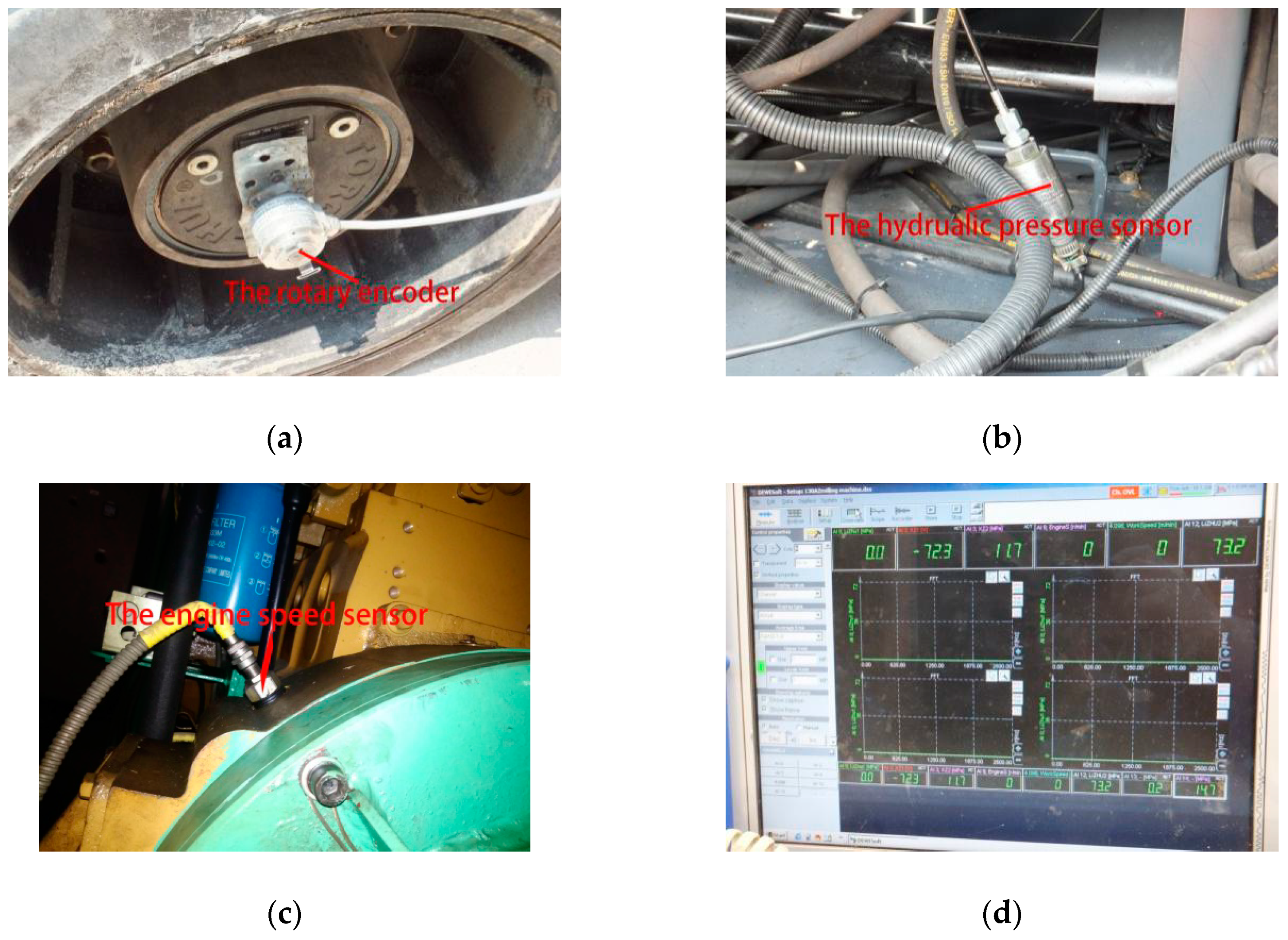
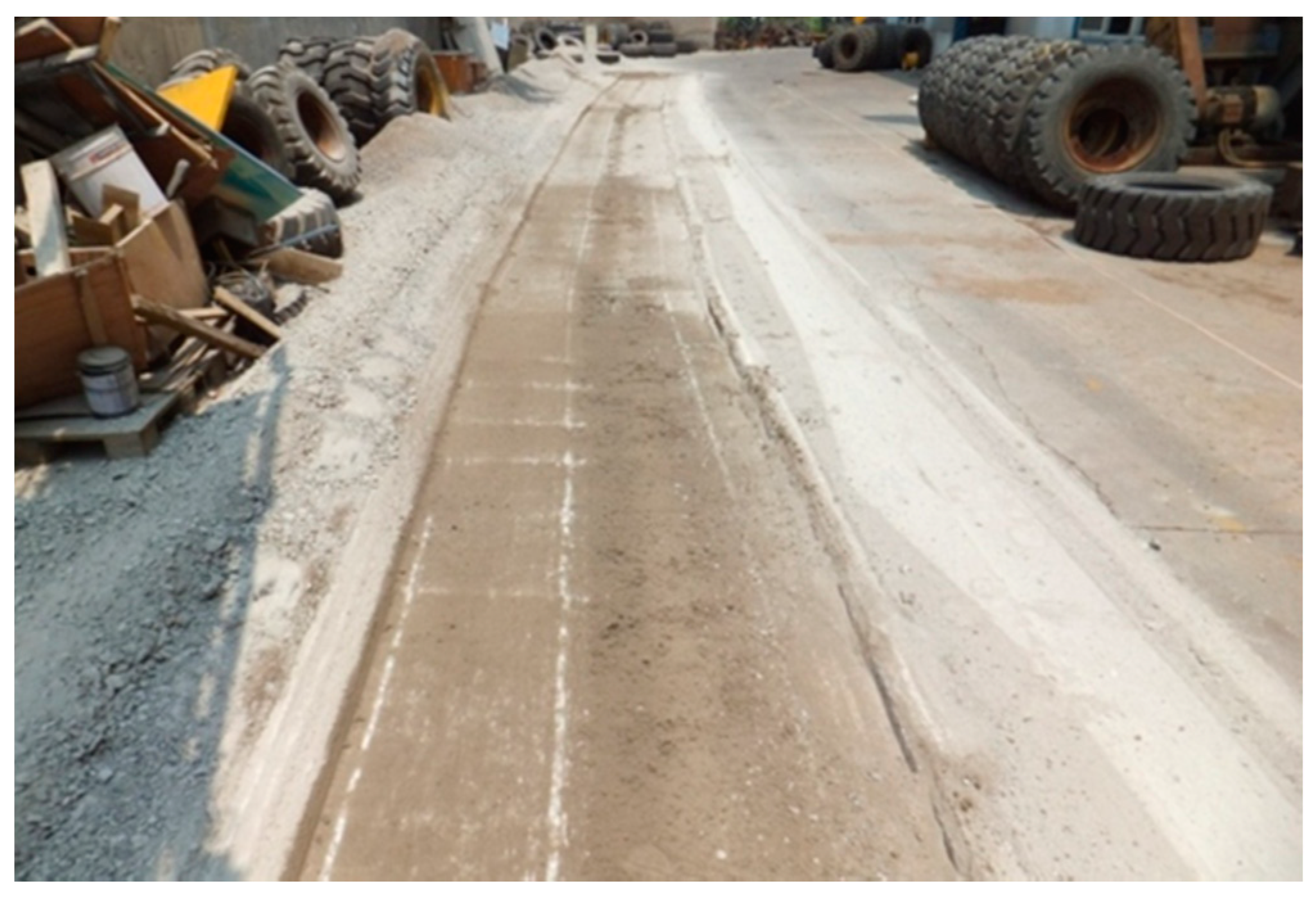
5.1. Field Test Setup

To validate the control effect of the supervised Hebb learning PID control algorithm presented in this work on the productivity of the cold milling machine, a field tested was conducted. The parameters of the tested cold milling machine are given as below. The mass of the machine is 20 tons. The milling depth of the cement concrete pavement is about 8 cm. The concrete strength is not well-distributed in the pavement. The engine throttle is at its maximum position, and the milling width of the machine is 1.3 m, the engine rated speed is 2000 rpm. To make full use of the engine power, the engine reference speed is 1,950 rpm, and the permissible error is 50 rpm. According to the field tests, the initial value of some control parameters are set respectively as ${\eta }_P$ = 2.6, ${\eta }_I$ = 1.5, ${\eta }_D$ = 0.7, $K_{u0}$ = 0.65. The sensors and data acquisition instrument are shown in Figure 9. Figure 10 is the picture of the machine working in the test field. Figure 11 shows the pavement milled by the cold milling machine.

The sensor used to test the work speed is an 11 bit rotary encoder with the resolution of 2048 pulses per revolution. The rotary encoder is provided by OMRON and the model of this encoder is E6C3-CWZ3EH 2048 P/R 1M. The sensor used to test the hydraulic pressure of the drive system is a pressure transducer, SENSOTEC Model Z serials. The measurement range of this pressure sensor is 0 to 15,000 psig. The engine speed sensor is a hall sensor which sends sinusoidal wave signals when the engine is running. The engine speed sensor is built-in the engine. The data acquisition instrument is DEWE-2010, and the sampling rate of the testing is set as 1000 Hz in this work.

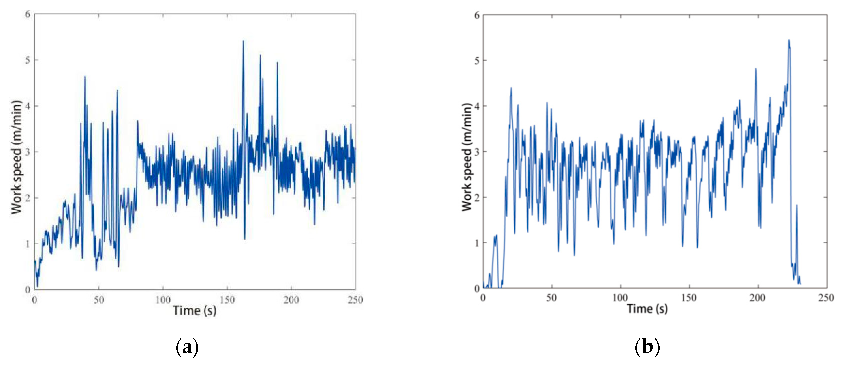
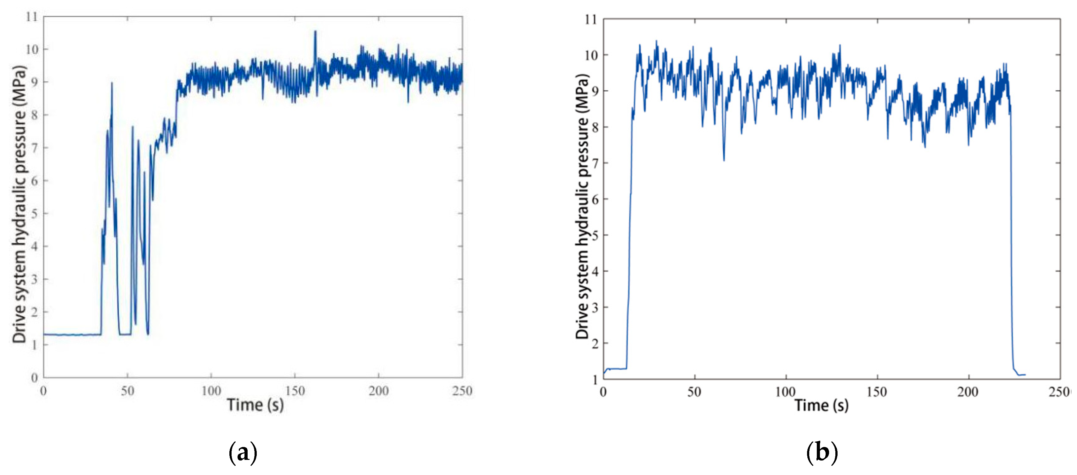
5.2. Field Test Results

The filed test is made up of two parts. In the first part, we operate the machine manually. When the machine works in the middle of the pavement, we choose the ‘AUTO’ mode of the machine, and then, the control system begins to work. The milling rotor of the machine gradually cuts into 8 cm depth of the pavement within the first 40 s of Figure 12a, Figure 13a and Figure 14a; the milling rotor entails enough power to meet the needs of consumers during this process, which make the engine speed decreases in Figure 12a. The hydraulic driving system is in a closed state at this point; the pressure of the hydraulic driving system in Figure 14a is the system back pressure. As the milling rotor of the machine gradually cuts into the depth of setting, the machine is slow-moving under the action of the level component of forces, so the work speed of the milling machine in Figure 13a is not zero. Fluctuations are mainly caused by the driver operation in Figure 12a, Figure 13a and Figure 14a. If the operator drives too fast the load increases sharply because of hard and rough usage over pavement. The driver needs to stop and loses time in a stationary position while powering up or reworking. Fluctuations are caused by local downhill pavement and the uneven distribution of pavement material within 161 s to 200 s in Figure 12a, Figure 13a and Figure 14a. When the machine works on the downhill pavement, the work speed of the milling machine will increase under the gravity along the ramp as the tractive force. Then, the forces of milling rotor increase with the depth of cut and feed rate, the milling rotor entails enough power to meet the needs of consumers during this process, which makes the engine speed decrease as in Figure 12a. The pressure of the hydraulic driving system in Figure 13a did not change significantly during this process, because the level component of forces and the gravity along the ramp as the tractive force was counteracting. The testing results are given in Figure 12, Figure 13 and Figure 14.

In Figure 12a, the engine is overloaded and the maximum fluctuation of the engine speed is 419 rpm when the machine is not equipped with the controller. The maximum engine speed is 2103 rpm; the machine is underloaded in this condition. When the machine is operated manually, the machine is often overloaded or underloaded. If the engine works on this condition, the output power is not at its desirable value. During this work process, the load of the machine with the fixed transmission ratio of the ground drive system is adjusted by the engine. If the machine load increases, the engine speed will go down. The work speed changes with the engine speed, i.e., the decline of the engine speed leads to the decline of the work speed. As a result the work load descends. When the work speed is at the certain value, the work load and the engine torque is in balance. This adjustment is a passive adaptation to the machine load for the system without the proposed controller.

As shown in Figure 12b, the fluctuation of the engine speed is 129 rpm, the engine average speed is 1954 rev/min and both values are near to the setting values and the engine is not seriously overloaded. When the engine speed deviates from the reference value for its overload or under load, the adaptive controller begins to adjust the displacement of the variable hydraulic pump to reduce or increase the machine work speed, i.e., when the machine is under load the controller will increase the work speed, and if the machine is under load the controller will reduce the work speed. This adjustment of the controller makes the work load descend or ascend and makes the engine work almost at its rated speed. Although the work speed in Figure 12b presents some fluctuation when the machine meets the great impulse load, the engine speed is almost at 1950 rpm mostly during the machine work process and the engine output power has increased near to its rated value. This adjustment is active adaptation to the machine load in this case.

Figure 13a shows that the average work-speed is 2.4 m/min when the machine is working without an adaptive controller and the work speed is adjusted manually or by the engine. Figure 13b shows that once the load of the machine changes, the controller will adjust the work speed. The average work speed is 2.766 m/min, which is 15.25% higher than that the machine without an adaptive controller. That is to say, the productivity of the machine increases 15.25%. The machine is not overloaded seriously and the engine speed is near to its rated value during its work process. The milled materials in the milling chamber are conveyed in time and the power consumption on mixing milled materials decreases. If the power consumption on mixing milled materials decreases and the average output power of the engine goes up, there will be more power, which can be used for the work of the machine. At the same time, the machine often works near to its rated conditions, and the dynamic performance and fuel economy of the engine is better than that with overloaded or underloaded conditions. When the machine works close to its rated conditions, the slip rate of the drive wheel is less than that in serious overloaded conditions, and the work speed will increase. When the machine is under loaded, the engine speed will go up, and then, the controller will increase the work speed to make the machine work near its rated condition. All these factors lead to a higher productivity of the machine with the developed controller in this work.

The tractive force of the milling force is reflected by the hydraulic pressure as shown in Figure 14. Analyzing Figure 13 and Figure 14, it is clear that the change trend of the hydraulic pressure is the same as the work speed. This is can be explained by Equation (9) which shows that the hydraulic pressure of the drive system increases with the speed of the hydraulic motor if the load is a constant.

6. Conclusions

In this work, a supervised Hebb learning single neuron adaptive PID controller has been developed and implemented for the power control of a cold milling machine. The power control process and the system model of a cold milling machine have been established to provide insight and guidance to the analysis, design and control of the power control system. The control algorithm and method has been validated by a field test. We can conclude that:

The cold machine with the adaptive power controller almost worked at its rated load. The minimum engine speed has achieved up to 1891 rev/min from 1684 rev/min. When the throttle is fixed at its maximum position, if the machine is overloaded, the minimum engine speed can reflect the overloaded level of the cold milling machine. The productivity of the cold milling machine with the control system increased by 15.25% compared to the machine without the control system.

This supervised Hebb learning single neuron adaptive PID control meets the need of the adaptive power control of the cold milling machine. The control system which uses this algorithm can increase the engine output power and productivity of a cold milling machine in practice.

References

1. Wang, Q. The Study on Milling Drum System of Road Cold Miller. Master’s Thesis, Dept. Mech. Eng., Xi’an University of Technology, Xi’an, China, 2006. [Google Scholar]
2. Guo, Y.; Duan, M. Computer Simulation of Load Fluctuation of Milling Cylinder of Pavement Planer. J. Hunan Univ. Sci. Technol. Nat. Sci. Ed. 2007, 24, 17–20. [Google Scholar]
3. Gu, H.; Jiao, S.; Xiao, A.C. Analysis and Test on Asphalt Milling Machine Cutting Load Characteristic. China J. Highw. Transp. 2012, 25, 154–158. [Google Scholar]
4. Wang, A.; Li, Z.; Yao, H. Discussion of automatic power apportioning of milling machine. Road Mach. Constr. Mech. 2005, 22, 34–36. [Google Scholar]
5. Long, J. Study on Working Principle and Power Allocation of Tracked Milling Machine. Road Mach. Constr. Mech. 2010, 27, 73–75. [Google Scholar]
6. Chen, Y.; Zou, X.; Yang, Y. Design of Digital Control System of Hydraulic Milling Machine. Mech. Eng. Autom. 2012, 19, 123–125. [Google Scholar]
7. Yuan, F. Design of Traveling Control System for Milling Machine Based on DSP. Road Mach. Constr. Mech. 2010, 27, 79–81. [Google Scholar]
8. Ma, P.; Hu, Y.; Zhang, X. Research on adaptive power control parameter of a cold milling machine. Simul. Model. Pract. Theory 2008, 16, 1136–1144. [Google Scholar]
9. Ma, P.; Hu, Y.; Zhang, Z. The dynamical model of a cold milling machine and its adaptive power control simulation. Simulation 2011, 87, 809–817. [Google Scholar]
10. Atherton, D.P. PID controller tuning. Comput. Control. Eng. J. 1999, 10, 44–50. [Google Scholar]
11. Nasr, M.B.; Chtourou, M. Neural network control of nonlinear dynamic systems using hybrid algorithm. Appl. Soft Comput. 2014, 24, 423–431. [Google Scholar]
12. Kumara, N.; Panwarb, V.; Sukavanam, N.; Sharma, S.P.; Borm, J.H. Neural network-based nonlinear tracking control of kinematic ally redundant robot manipulators. Math. Comput. Model. 2011, 53, 1889–1901. [Google Scholar]
13. Ge, S.S.; Hong, F.; Lee, T.H. Adaptive neural network control of nonlinear systems with unknown time delays. IEEE Trans. Autom. Control. 2003, 48, 2004–2010. [Google Scholar]
14. Yang, Q.; Yang, Z.; Sun, Y. Universal Neural Network Control of MIMO Uncertain Nonlinear Systems. IEEE Trans. Neural Netw. Learn. Syst. 2012, 23, 1163–1169. [Google Scholar]
15. Baloochy, B. A Robust Approach in Nonlinear Fuzzy Control of Chemical Process. Chem. Eng. Res. Bull. 2013, 16, 45–60. [Google Scholar]
16. Sofianos, N.A.; Boutalis, Y.S. Robust adaptive multiple models based fuzzy control of nonlinear systems. Neurocomputing 2016, 173, 1733–1742. [Google Scholar]
17. Harb, A.M.; Smadi, I.A. Tracking control of DC motors via mimo nonlinear fuzzy control. Chaos Solitons Fractals 2009, 42, 702–710. [Google Scholar]
18. He, Z.; Ji, X. Nonlinear robust control of integrated vehicle dynamics. Veh. Syst. Dyn. 2012, 50, 247–280. [Google Scholar]
19. Tian, B.; Fan, W.; Zong, Q.; Wang, J.; Wang, F. Nonlinear robust control for reusable launch vehicles in reentry phase based on time-varying high order sliding mode. J. Frankl. Inst. 2013, 350, 1787–1807. [Google Scholar]
20. Raffo, G.V.; Ortega, M.G.; Rubio, F.R. Robust Nonlinear Control for Path Tracking of a Quad-Rotor Helicopter. Asian J. Control. 2015, 17, 142–156. [Google Scholar]
21. Isidori, A.; Marconi, L.; Serrani, A. Robust nonlinear motion control of a helicopter. IEEE Trans. Autom. Control. 2003, 48, 413–426. [Google Scholar]
22. Abdeddaim, S.; Betka, A.; Drid, S.; Becherif, M. Implementation of MRAC controller of a DFIG based variable speed grid connected wind turbine. Energy Convers. Manag. 2014, 79, 281–288. [Google Scholar]
23. Mirkin, B.; Gutman, P.-O.; Shtessel, Y. Coordinated decentralized sliding mode MRAC with control cost optimization for a class of nonlinear systems. J. Frankl. Inst. 2012, 349, 1364–1379. [Google Scholar]
24. Zilletti, M.; Elliott, S.J.; Gardonio, P.; Rustighi, E. Experimental implementation of a self-tuning control system for decentralized velocity feedback. J. Sound Vib. 2012, 331, 1–14. [Google Scholar]
25. Wang, R.; Chen, L.; Wang, D. Self-tuning Control on Integrated System of EPS and SAS Based on Pole Placement. Procedia Eng. 2011, 16, 271–277. [Google Scholar]
26. Yao, H. The Hydraulic Dynamics and Control Mechanism of Construction Vehicles; China Communications Press: Beijing, China, 2006. [Google Scholar]
27. Hu, Y.; Ma, P.; Zhang, X. Modelling and simulating of cold milling machine. J. Chang’an Univ. Nat. Sci. Ed. 2008, 28, 92–95. [Google Scholar]
28. Galichet, S.; Foulloy, L. Fuzzy controllers: synthesis and equivalences. IEEE Trans. Fuzzy Syst. 1995, 3, 140–148. [Google Scholar]
29. Ding, J.; Xu, Y. Single Neuron Adaptive PID Controller and its Applications. Control Eng. China 2004, 11, 27–30. [Google Scholar]
30. Yadav, R.; Kalra, P.K.; John, J. Time series prediction with single multiplicative neuron model. Appl. Soft Comput. 2007, 7, 1157–1163. [Google Scholar]
31. Cai, Z. Intelligent Control, 2nd ed.; Publishing House of Electronics Industry: Beijing, China, 2004. [Google Scholar]
32. He, L.; Wan, Z.; Cheng, L.; Liao, X. Simulink simulation of single neuron PID and smith predictive control based on the s-Function. In Proceedings of the 2013 Third International Conference on IMCCC, Shenyang, China, 21–23 September 2013; pp. 1548–1551. [Google Scholar]
33. Zhao, X.; Jiao, Y. Single Neuron Self-Adaptive PSD Control and Its Application in Reheat Steam Temperature Control System. Chin. Soc. Elec. Eng. 2001, 21, 93–96. [Google Scholar]
34. Cheng, Q.; Wan, D.; Huang, L. The Single Neuron Adaptive PID/PSD Controller of Ship Autopilot. J. Southeast Univ. 1997, 27, 133–137. [Google Scholar]
35. Astrom, K.J.; Hagglund, T. PID Controllers: Theory, Design and Tuning, 2nd ed.; Instrument Society of America: Research Triangle Park, NC, USA, 1995. [Google Scholar]
36. Jiao, S. Research on the Hydraulic Drive and Control Systems of an Asphalt Concrete Spreader. Ph.D Thesis, Dept. Mech. Eng. Chang’an University, Xi’an, China, 2002; pp. 36–51. [Google Scholar]
37. Lei, T. New Manual of Hydraulic Engineering; Beijing Institute of Technology Press: Beijing, China, 1998; pp. 3–6. [Google Scholar]
38. Zeng, W.; Zhao, M.; He, T. Working performance for asphalt road plane milling machine. J. Chang’an Univ. Nat. Sci. Ed. 2004, 24, 58–61. [Google Scholar]
Figure 1. Structure of a cold milling machine.
Applsci 10 02516 g001
Figure 2. Working process of cold milling machine.
Applsci 10 02516 g002
Figure 3. The diagram of the power control process.
Applsci 10 02516 g003
Figure 4. Structure of the adaptive power control of a cold milling machine.
Applsci 10 02516 g004
Figure 5. The interferential load curve.
Applsci 10 02516 g005
Figure 6. The engine speed curves.
Applsci 10 02516 g006
Figure 7. The engine output power curves.
Applsci 10 02516 g007
Figure 8. The machine work speed curves.
Applsci 10 02516 g008
Figure 9. The sensors and data acquisition instrument: (a) the work speed sensor; (b) the drive hydraulic pump pressure sensor; (c) the engine speed sensor; (d) the data acquisition instrument.
Applsci 10 02516 g009
Figure 10. The field test of the cold milling machine.
Applsci 10 02516 g010
Figure 11. The milled cement pavement.
Applsci 10 02516 g011
Figure 12. Engine speeds of (a) proportional-integral-derivative (PID) controller and (b) the proposed adaptive power controller.
Applsci 10 02516 g012
Figure 13. Work speed of the milling machine: (a) PID controller and (b) with the proposed controller.
Applsci 10 02516 g013
Figure 14. The drive system hydraulic pressure: (a) PID controller and (b) the proposed controller.
Applsci 10 02516 g014