Featured Application
In this study, an innovative model for infrared image deblurring under Gaussian noise is proposed by exploring the sparsity of high-order total variation, leading to enormous progress in image recovery performance.
Abstract
The quality of infrared images is affected by various degradation factors, such as image blurring and noise pollution. Anisotropic total variation (ATV) has been shown to be a good regularization approach for image deblurring. However, there are two main drawbacks in ATV. First, the conventional ATV regularization just considers the sparsity of the first-order image gradients, thus leading to staircase artifacts. Second, it employs the L1-norm to describe the sparsity of image gradients, while the L1-norm has a limited capacity of depicting the sparsity of sparse variables. To address these limitations of ATV, a high-order total variation is introduced in the ATV deblurring model and the Lp-pseudonorm is adopted to depict the sparsity of low- and high-order total variation. In this way, the recovered image can fit the image priors with clear edges and eliminate the staircase artifacts of the ATV model. The alternating direction method of multipliers is used to solve the proposed model. The experimental results demonstrate that the proposed method does not only remove blurs effectively but is also highly competitive against the state-of-the-art methods, both qualitatively and quantitatively.
1. Introduction
Thermal infrared imagers can create images of targets when they are completely dark and far away. Moreover, the disguised targets and high-speed moving targets can also be detected in thick smoke screens and clouds. Thus, thermal infrared imagers are widely used in military and civilian applications. Consequently, users prefer higher requirements for the quality of infrared images acquired from thermal infrared imagers. The principle of infrared image generation [1,2,3] is as follows. The object whose temperature is above absolute zero in nature radiates infrared rays outward. Based on the infrared radiation, the infrared system employs a sensor to convert infrared radiation into electricity signals. After signal processing, it presents the corresponding visible light image on the display medium. As the infrared imaging system is more complex than the natural imaging system, the infrared images suffer from relatively more degradation, such as Gaussian blurring, motion blurring, and noise pollution. Therefore, deblurring infrared images plays a significant role in an infrared imaging system. Researchers have proposed some infrared image deblurring methods, for instance, the quaternion and high-order overlapping group sparse total variation model [4], the total variation with overlapping group sparsity and Lp quasinorm model [5], and the quaternion fractional-order total variation with Lp quasinorm model [6].
The total variation (TV) [7] model is simple and effective for image deblurring. However, it assumes the images to be piecewise constants, thus resulting in staircase artifacts [8]. Several TV-based restoration methods have been proposed to address the issue of staircase artifacts. Generally, these extensions are mainly divided into two categories, local information-based TV extension and non-local based TV extension. The local information-based TV model relies on exploring the total variation in a limited local area. On the contrary, non-local information-based TV models explore patch similarity by searching in the entire image. Concerning local information-based TV extension, Sroisangwan [9] proposed a new higher-order regularization for removing noise. Oh et al., [10] proposed a non-convex hybrid TV (Hybrid TV) model by introducing high-order TV. Similarly, Liu et al., [11] assumed the first-order and second-order gradients to be hyper-Laplacian distributions and proposed a constrained non-convex hybrid TV model for edge-preserving image restoration. Likewise, Zhu et al., [12] proposed an effective hybrid regularization model based on the second-order total generalized variation and wavelet frame. Recently, Lanza et al., [13] proved that non-convex regularizations can promote sparsity more effectively than convex regularizations. Thus, by considering non-convex tools for depicting sparsity, Anger et al., [14] proposed blind image deblurring using the L0 gradient prior. Yang et al., [15] proposed a weighted-l1-method noise regularization for image deblurring. Based on overlapping group sparsity, Selesnick et al., [16], Liu et al., [17], Liu et al., [18,19], Shi et al., [20] and Wang et al., [21] proposed image reconstruction schemes to further minimize staircase artifacts. Adam et al., [22,23] combined second-order non-convex TV and non-convex higher-order total variation with overlapping group sparse regularization to remove staircase artifacts. By taking advantage of neighbor information, Cheng et al., [24] proposed a four-directional TV denoising method. Combining the Lp-quasinorm shrinkage with four-directional TV, Liu et al., [6] extended anisotropic total variation (ATV) to a quaternion fractional TV using the Lp-quasinorm (FTV4Lp) model. The aforementioned models mainly rely on local image information. In contrast, by considering non-local information, Wang et al., [25] used a non-local data fidelity term to build a denoising model. Xu [26] adopted non-local TV models to regularize the solution to the image recovery optimization problem. Nasonov et al., [27] combined the block-matching and 3D (BM3D) filtering with generalized TV to deblur images. By considering the similarity of nonlocal patches, Liu et al., [28] proposed a block-matching TV regularization.
The Lp-pseudonorm is an emerging tool that is used for depicting sparse variables and has been applied in several signal-processing applications. Woodworth et al., [29] demonstrated that Lp shrinkage is superior to soft threshold shrinkage in recovering sparse signals. Recently, Lp shrinkage has been applied to numerous fields, for example, Liu et al., [5] proposed a method using the Lp-quasinorm instead of the L1-norm for infrared image deblurring with the overlapping group sparse TV method. Chen et al., [30] presented a sparse time-frequency representation model using the Lp-quasinorm constraint, this model is capable of fitting the sparsity prior to the frequency domain. Li et al., [31] extended the ATV model to the anisotropic total variation Lp-quasinorm shrinkage (ATpV) model for impedance inversion. Zhao et al., [32] put forward the Lp-norm-based sparse regularization model for license plate deblurring.
Inspired by the aforementioned studies, we propose a model that combines the first-order and high-order ATV with Lp-pseudonorm shrinkage to construct a new image-deblurring model, hereafter referred to as HTV-Lp. The proposed model addresses the following limitations of the conventional TV model: (1) staircase artifacts; and (2) the limited capability of the L1-norm to depict the sparsity of sparse variables. To realize the new HTV-Lp model, the alternating direction method of multipliers (ADMM) framework [33] was adopted. Fast Fourier transform (FFT) was used to improve the algorithm efficiency. To validate the newly proposed HTV-Lp model, experiments were performed to compare its performance with existing models including ATV [7], isotropic total variation (ITV) [34], ATpV [31], FTV4Lp [6] and non-convex hybrid TV (Hybrid TV) [10]. Objective indicators of the six methods were evaluated, such as the peak signal-to-noise ratio (PSNR) [35], structural similarity (SSIM) [36], and gradient magnitude similarity deviation (GMSD) [37]. The major contributions that have led to significant improvements in the quality of deblurred infrared images are as follows: (1) considering the sparsity of a high-order gradient field based on the ATV model; (2) introducing Lp-pseudonorm shrinkage to express the sparsity of a first-order and high-order gradient field; (3) combining first-order TV and high-order TV with Lp-pseudonorm shrinkage organically; (4) adjusting the parameters in the model separately.
This paper is organized as follows: Section 2 presents the ATV deblurring model. The HTV-Lp model proposed in this paper is described in Section 3. The algorithm for solving the HTV-Lp model is presented in Section 4. Next, the publicly available datasets, evaluation metrics, results of the extensive experiments conducted for evaluation of the six models, and experimental analysis are presented in Section 5. Finally, Section 6 concludes the paper.
2. Traditional Anisotropic Total Variation (ATV) Model
The ATV deblurring model [38] is described as follows:
The Gaussian blurring kernel is represented by a point spread function [5], represents the original image, and represents the observed image with noise. is the fidelity term, is the prior term, and the balance factor is used to balance the prior and fidelity terms.
where represents the two-dimensional convolution kernels, describes information in the horizontal direction of the image, while describes the information in the vertical direction of the image.
3. Proposed Model
Because the pixel information is not fully considered in the traditional ATV model, only the information of the first-order gradient is considered. To enhance the deblurring effect, the traditional ATV model is extended to the high-order TV model, which considers the first-order gradient information, and adds the high-order gradient information to the prior term. Figure 1 depicts the contour maps that highlight the advantage of Lp-pseudonorms. The contours of the L1-norm, L2-norm and Lp-pseudonorm are depicted in Figure 1a–c. The L1-norm and L2-norm can be expressed as and , respectively; whereas, the Lp-pseudonorm is defined in the following paper. In Figure 1, the dotted lines represent the fidelity term, while the solid blue lines represent the contours of the prior item. The red dots represent the intersection of the dotted line and the solid line, while the intersections with the axes represent the better sparseness of the image gradients. It is also observed that the Lp-pseudonorm provides a greater degree of freedom compared with L1-norm and L2-norm, which can better depict the sparsity of the image gradients. Therefore, the Lp-pseudonorm was added to the prior terms to improve the robustness of the image gradients.
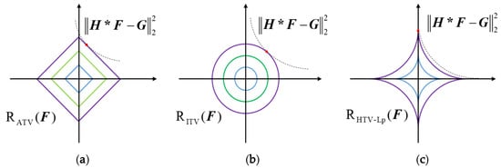
Figure 1.
Contour maps of different norms. (a) L1-norm, (b) L2-norm, (c) Lp-pseudonorm ().
The high-order gradient information and Lp-pseudonorm were introduced to increase the accuracy of the prior knowledge, thereby preserving the edge of the image while suppressing the influence of the small edge on the estimation of the blurring core. Therefore, the proposed high-order total variation with Lp-pseudonorm shrinkage (HTV-Lp) model is defined as follows:
where , the Lp-norm is defined as , while the Lp-pseudonorm is defined as , and are the balance parameters.
4. Solver by Alternating Direction Method of Multipliers (ADMM)
4.1. The Proposed Model Solution Based on the Alternating Direction Method of Multipliers
To resolve the HTV-Lp model defined by Equation (3), the ADMM framework [33,39] is used. The complex problem was transformed into several simple decoupled sub-problems using variable substitution. The split variables can be defined as . The original problem is transformed into the following equations:
where .
According to the ADMM principle, dual variables are introduced. The problem shown in Equation (4) can be converted into an unconstrained extended Lagrange function:
where represents the inner product of and , and is the penalty factor of the quadratic penalty function.
4.2. F Sub-Problem Solving
The sub-function of the sub-problem of is written as follows,
A supplement to Equation (6) can be formulated as follows,
The sub-function then becomes:
The Fourier transform is performed on the above expression to obtain the frequency domain representation and transform Equation (8) into the following equation:
where the symbol represents the point multiplication operation and represents the spectrum of .
The derivative of Equation (9) to is as follows,
Let and be defined as Equations (11) and (12), respectively,
Then, according to Equation (10), is defined as follows,
where denotes fast inverse Fourier transform.
4.3. Sub-Problem Solving
The objective function of the subproblem is:
We adopted Lp-pseudonorm shrinkage to solve the Equation (14). In contrast to Wang et al., [21] where the value of was the same, we separated the values of different gradients and directions of the image. The advantage of this operation lies in the fact that it can improve the performance of the deblurring image as described in Section 5.3. Lp-pseudonorm shrinkage is defined as . According to the Lp-pseudonorm shrinkage rule, can be updated as follows,
Similarly, we have:
4.4. Sub-Problem Solving
The objective function of the sub-problem of can be written as follows,
According to the mountain climbing method [40],
where γ is the learning rate.
Table 1 presents the pseudocode of HTV-Lp for infrared image deblurring.

Table 1.
The pseudo-code of the proposed method.
where represents the threshold.
5. Experimental Results and Analysis
5.1. Experimental Environment
To demonstrate the superiority of the proposed HTV-Lp model, Figure 2 shows eight different test images downloaded from the publicly available datasets found in http://adas.cvc.uab.es/elektra/datasets/far-infra-red/, and http://www.dgp.toronto.edu/~nmorris/data/IRData/. Infrared images of http://adas.cvc.uab.es/elektra/datasets/far-infra-red/were obtained using an infrared camera (PathFindIR Flir camera) with 19-mm focal length lens. The size of the “Store.BMP” is 506 × 408 and that of the rest images are 384 × 288. The Gaussian blur and motion blur kernels are generated by MATLAB functions. For example, MATLAB function “fspecial” (‘gaussian’, B × B × σ) generates a B × B Gaussian blur kernel with a standard deviation of σ. For convenience, the kernel is referred to as (G, B, B, σ). “fspecial” (‘motion’, L, θ) generates a motion blur kernel with a motion displacement of L and motion angle of θ, which is referred to as (M, L, θ) for convenience. Furthermore, Gaussian noise standard deviations of 1, 3, and 5 are used.
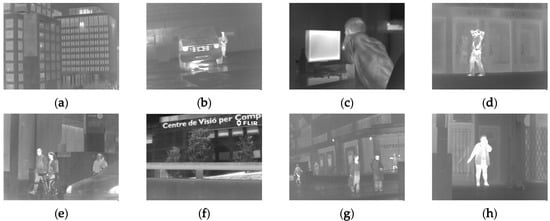
Figure 2.
Test images. (a) Building.BMP; (b) Car.BMP; (c) Figure.BMP; (d) Man.BMP; (e) People.BMP; (f) Store.BMP; (g) Street.BMP; and (h) Woman.BMP.
5.2. Evaluation Metrics
The main comparison evaluation metrics considered in this study are the PSNR, SSIM, and GMSD, which are expressed in Equations (19)–(21), respectively:
where and refer to the original image and the restored image, respectively. and are the average of the sum of the images, and , represent the variance of and , respectively. Here, k1 and k2 are used to ensure that the SSIM expression is non-zero; in this experiment, k1 is set as 0.01 and k2 as 0.03.
where,
where and refer to the gradient amplitude of the image in the horizontal and vertical directions, respectively, and is a constant of small value to guarantee that the denominator is a non-zero number.
Larger PSNR values and smaller GMSD values correspond to better image recovery quality. The range of SSIM is (0, 1), where higher values indicate better deblurring performance. The iterative stop condition in the algorithm can be expressed as follows,
where is set to be .
5.3. The Sensitivity of the Parameters
The parameters should be properly selected. We try each parameter tentatively until the iterated image is properly recovered. The ranges of each parameter are determined empirically as . The parameters are adjusted by traversing these ranges with a step size of 0.01. When PSNR achieves a maximum value, the corresponding parameter values are selected as the optimal ones. Figure 3 depicts the effect of on PSNR during the adjustment. Notably, when the PSNR reaches its maximum, the optimal selections of vary, hence, it is effective to adjust these parameters separately.
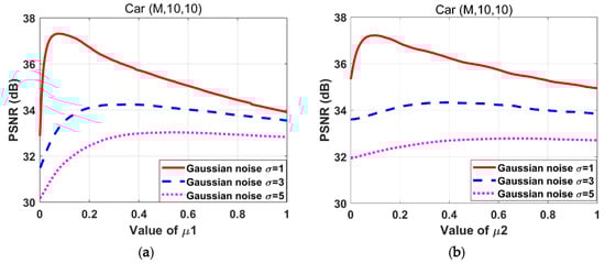
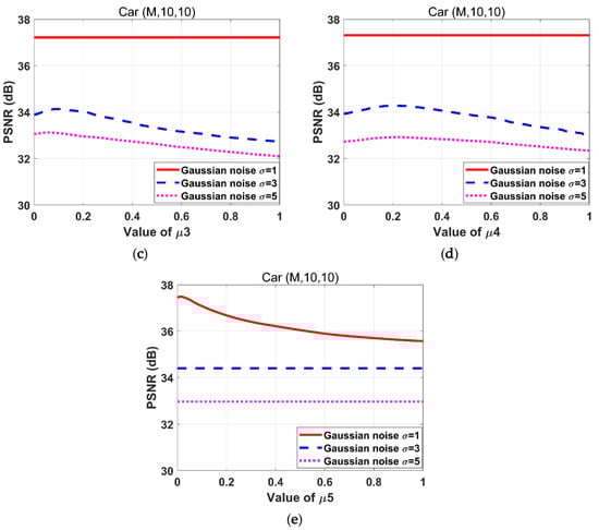
Figure 3.
Effects of variations on the peak signal-to-noise ratio (PSNR) for the “Car” images degraded by the motion blur kernel (M, 10, 10) with Gaussian noise standard deviations 1, 3, and 5 respectively. (a) ; (b) ; (c) ;(d) ; (e) .
Figure 4 depicts the effect of variations in on PSNR during the adjustment. When the is too large, the image gradient sparsity is not sufficiently strong. However, if is too small, the image gradients become too sparse. Thus, the value of should be adjusted until the image recovery is satisfactory. As shown in Figure 4, the values of are different when PSNR reaches the maximum value under the same experimental conditions. Therefore it is effective to separate the of different gradients and directions of image.
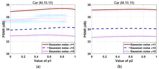
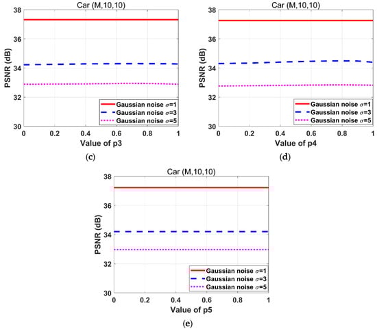
Figure 4.
Effects of variations on the PSNR for the “Car” images degraded by the motion blur kernel (M, 10, 10) with Gaussian noise standard deviations 1, 3, and 5 respectively. (a) ; (b) ; (c) ; (d) ; (e) .
5.4. Comparison of the Deblurring Performance
The parameters of the six algorithms are adjusted by the traversal to achieve the best deblurring indicators. The test results for the different images are presented in Table 2 and Table 3, where the values in bold refer to the optimal indicator values. Table 2 presents the deblurred results obtained by the six different models for degraded images with Gaussian blur (G, 5, 5, 7) and Gaussian noise standard deviations of 1, 3, and 5, respectively. Table 3 presents the results obtained by the six different models for degraded images with motion blur (M, 10, 10) and Gaussian standard deviations of 1, 3, and 5, respectively. Figure 5 depicts the changes in the methods in terms of the evaluation metrics with respect to the increase in the iteration number.
Table 2.
Evaluation metrics of the six algorithms for various images with motion blur (M, 10, 10) with a Gaussian noise standard deviation (SD) of 1, 3, and 5.
Table 3.
Evaluation metrics of the six algorithms for various images with Gaussian blur (G, 5, 5, 7) with a Gaussian noise standard deviation (SD) of 1, 3, and 5.
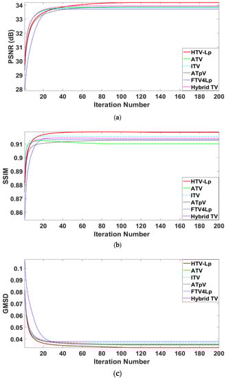
Figure 5.
Dynamic iterative curves with different evaluation metrics. (a); (b); (c) are figures illustrating effects for the degraded “Car” image with the motion blur kernel (M, 10, 10) and Gaussian noise standard deviation of 3 on PSNR, structural similarity (SSIM), gradient magnitude similarity deviation (GMSD), respectively.
The performance of the proposed method, illustrated intuitively in Figure 5, and Table 2 and Table 3, can be summarized as follows: (1) The performance indicators obtained by the HTV-Lp model are higher than all the other models, thereby demonstrating that the proposed method has better deblurring and denoising effects. (2) Observed from Table 2 when restoring the eight degraded images with the motion blur kernel (M, 10, 10) and Gaussian noise standard deviation of 1–5, the HTV-Lp model shows average PSNR values 0.584 dB higher than those of the ATV method, 0.536 dB higher than those of the ITV method, 0.389 dB higher than those of the ATpV method, 0.575 dB higher than those of the FAV4Lp method, and 0.100 dB higher than those of the Hybrid TV method. (3) Observed from Table 3 when restoring the eight degraded images with Gaussian blur kernel (G, 5, 5, 7) and Gaussian noise standard deviation of 1–5, the HTV-Lp model shows average PSNR values 0.531 dB higher than those of the ATV method, 0.391 dB higher than those of the ITV method, 0.300 dB higher than those of the ATpV method, 0.589 dB higher than those of the FAV4Lp method, and 0.175 dB higher than those of the Hybrid TV method. Hence, we conclude that the high-order gradients sparsity of the image is helpful for image recovery and Lp-pseudonorm is better than L1-norm.
5.5. Comparison of Visual Effects
The deblurring results for the “Store” are depicted in Figure 6. To better exhibit the effects of the six algorithms, a part of “Store” details in the red rectangles was enlarged. It can be seen that the HTV-Lp model minimized the noise while simultaneously reliving the staircase artifacts in slanted and smooth regions of the image during image deblurring. In addition, the Lp-pseudonorm can depict the sparsity of processed variables more precisely compared to the L1-norm. Figure 7 depicts the single columns extracted by original image, degraded image and deblurring images of ATV, ITV, ATpV, FTV4Lp, Hybrid TV, HTV-Lp. It is found that the HTV-Lp achieves the flattest curve among the compared methods.
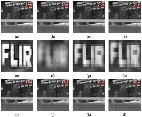
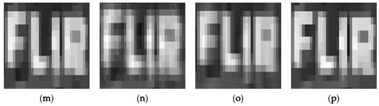
Figure 6.
Comparison of the visual effects. (a) is the original “Store” image; (b) is the degraded image with Gaussian blur (G, 5, 5, 7) and Gaussian noise standard deviation of 5; (c,d,i–l) are the deblurring results of ATV, ITV, ATpV, FTV4Lp, Hybrid TV, and HTV-Lp methods, respectively; (e–h,m–p) show the magnified details from the rectangles in (a–d,i–l), respectively.
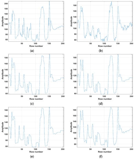
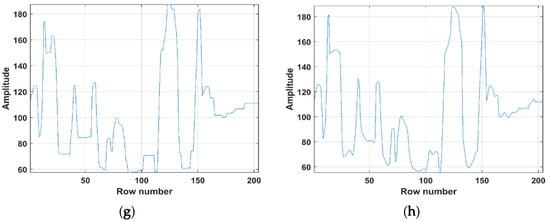
Figure 7.
Comparison of drawing charts. (a–h) are the drawing charts of original “Store” image, degraded “Store” image with Gaussian blur (G, 5, 5, 7) and Gaussian noise standard deviation of 5, deblurring results of ATV, ITV, ATpV, FTV4Lp, Hybrid TV, and HTV-Lp methods, respectively.
5.6. Comparison of Computing Time
Figure 8 shows comparison of computing times of different deblurring methods. Although our method, HTV-Lp, is slower than the others, the computing time is within 3.5 s, thus it is effective to employ convolution and the FFT theorem to avoid large computational complexity.
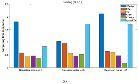
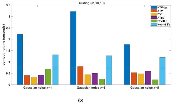
Figure 8.
Comparison of computing times of different deblurring methods. (a) degraded “Building” image with Gaussian blur (G, 5, 5, 7) and (b) degraded “Building” image with motion blur (M, 10, 10).
6. Discussion and Conclusions
Deblurring infrared images plays a significant role in an infrared imaging system. To improve the performance of deblurring images, the propoed HTV-Lp model combines first-order and high-order gradients of images with Lp-pseudonorm shrinkage. The ADMM algorithm is used to split the proposed model into several decoupled sub-problems. In the process of solving thee problems, the convolution and FFT theorem are applied to image deblurring to avoid large computational complexity. The comparison of HTV-Lp with existing ATV, ITV, ATpV, FTV4Lp, and Hybrid TV models shows that HTV-Lp obtained the average highest PSNR and SSIM and lowest GMSD values of all methods and successfully mitigated staircase artifacts.
A limitation of this study is that non-local patch similarity is not fully considered in the proposed model. Additionally, there is room for further improvement with regard to the speed of the HTV-Lp algorithm within the framework of the accelerated ADMM. Thus, in our future work, we will focus on improving the performance and efficiency of the proposed method.
Author Contributions
Conceptualization, J.Y. and Y.C.; Data curation, J.Y.; Formal analysis, J.Y.; Funding acquisition, Y.C.; Investigation, J.Y.; Methodology, J.Y.; Project administration, J.Y.; Resources, J.Y.; Software, J.Y.; Supervision, Y.C. and Z.C.; Validation, J.Y.; Visualization, J.Y.; Writing original draft, J.Y.; Writing—review and editing, Y.C. and Z.C. All authors have read and agreed to the published version of the manuscript.
Funding
This research was funded by Educational and Research Project for Young and Middle-aged Teachers of Education Department of Fujian Provincial (JAT190378); Fujian Province Major Teaching Reform Project (FBJG20180015); The Foundation of President of Minnan Normal University (KJ19019), and the Teaching Reform Project of Minnan Normal University (JG201918).
Acknowledgments
Thanks to X.L. of the University of Electronic Science and Technology of China for sharing the FTV4Lp code.
Conflicts of Interest
The authors declare no conflict of interest. The funders had no role in the design of the study; in the collection, analyses, or interpretation of data; in the writing of the manuscript; or in the decision to publish the results.
References
- Wang, X.W.; Shen, T.S.; Zhou, X.D. Simulation of the Sensor in the Infrared Image Generation. Semicond. Optoelectron. 2004, 25, 317–319. [Google Scholar]
- Choi, J.-H.; Shin, J.-M.; Kim, J.-H.; Kim, T.-K. Study on Infrared Image Generation for Different Surface Conditions with Different Sensor Resolutions. J. Soc. Nav. Arch. Korea 2010, 47, 342–349. [Google Scholar] [CrossRef]
- Norton, P.R. Infrared image sensors. Opt. Eng. 1991, 30, 1649. [Google Scholar] [CrossRef]
- Liu, X.; Chen, Y.; Peng, Z.; Wu, J. Infrared Image Super-Resolution Reconstruction Based on Quaternion and High-Order Overlapping Group Sparse Total Variation. Sensors 2019, 19, 5139. [Google Scholar] [CrossRef] [PubMed]
- Liu, X.; Chen, Y.; Peng, Z.; Wu, J. Total variation with overlapping group sparsity and Lp quasinorm for infrared image deblurring under salt-and-pepper noise. J. Electron. Imaging 2019, 28, 043031. [Google Scholar] [CrossRef]
- Liu, X.; Chen, Y.; Peng, Z.; Wu, J.; Wang, Z. Infrared Image Super-Resolution Reconstruction Based on Quaternion Fractional Order Total Variation with Lp Quasinorm. Appl. Sci. 2018, 8, 1864. [Google Scholar] [CrossRef]
- Rudin, L.I.; Osher, S.; Fatemi, E. Nonlinear total variation based noise removal algorithms. Phys. D Nonlinear Phenom. 1992, 60, 259–268. [Google Scholar] [CrossRef]
- Hajiaboli, M.R. An Anisotropic Fourth-Order Diffusion Filter for Image Noise Removal. Int. J. Comput. Vis. 2010, 92, 177–191. [Google Scholar] [CrossRef]
- Sroisangwan, P.; Chumchob, N. A Higher-Order Variational Model for Image Restoration and Its Medical Applications; Silpakorn University: Bangkok, Thailand, 2020. [Google Scholar]
- Oh, S.; Woo, H.; Yun, S.; Kang, M. Non-convex hybrid total variation for image denoising. J. Vis. Commun. Image Represent. 2013, 24, 332–344. [Google Scholar] [CrossRef]
- Liu, R.W.; Wu, D.; Wu, C.-S.; Xu, T.; Xiong, N. Constrained Nonconvex Hybrid Variational Model for Edge-Preserving Image Restoration. In Proceedings of the 2015 IEEE International Conference on Systems, Man, and Cybernetics, Kowloon, China, 9–12 October 2015; pp. 1809–1814. [Google Scholar]
- Zhu, J.; Li, K.; Hao, B. Image Restoration by Second-Order Total Generalized Variation and Wavelet Frame Regularization. Complexity 2019, 2019, 1–16. [Google Scholar] [CrossRef]
- Lanza, A.; Morigi, S.; Selesnick, I.W.; Sgallari, F. Sparsity-Inducing Nonconvex Nonseparable Regularization for Convex Image Processing. SIAM J. Imaging Sci. 2019, 12, 1099–1134. [Google Scholar] [CrossRef]
- Anger, J.; Facciolo, G.; Delbracio, M. Blind Image Deblurring using the l0 Gradient Prior. Image Process. Line 2019, 9, 124–142. [Google Scholar] [CrossRef]
- Yang, C.; Wang, W.; Feng, X.; Liu, X. Weighted-l1-method-noise regularization for image deblurring. Signal Process. 2019, 157, 14–24. [Google Scholar] [CrossRef]
- Selesnick, I.; Chen, P.-Y. Total variation denoising with overlapping group sparsity. In Proceedings of the 2013 IEEE International Conference on Acoustics, Speech and Signal Processing, Vancouver, BC, Canada, 26–31 May 2013; pp. 5696–5700. [Google Scholar]
- Liu, G.; Huang, C.; Liu, J.; Lv, X.-G. Total Variation with Overlapping Group Sparsity for Image Deblurring under Impulse Noise. PLoS ONE 2015, 10, e0122562. [Google Scholar] [CrossRef] [PubMed]
- Liu, J.; Huang, C.; Selesnick, I.; Lv, X.-G.; Chen, P.-Y. Image restoration using total variation with overlapping group sparsity. Inf. Sci. 2015, 295, 232–246. [Google Scholar] [CrossRef]
- Liu, J.; Huang, C.; Liu, G.; Wang, S.; Lv, X.-G. Total variation with overlapping group sparsity for speckle noise reduction. Neurocomputing 2016, 216, 502–513. [Google Scholar] [CrossRef]
- Shi, M.; Han, T.; Liu, S. Total variation image restoration using hyper-Laplacian prior with overlapping group sparsity. Signal Process. 2016, 126, 65–76. [Google Scholar] [CrossRef]
- Wang, L.; Chen, Y.; Lin, F.; Chen, Y.; Yu, F.; Chen, Y. Impulse Noise Denoising Using Total Variation with Overlapping Group Sparsity and Lp-Pseudo-Norm Shrinkage. Appl. Sci. 2018, 8, 2317. [Google Scholar] [CrossRef]
- Adam, T.; Paramesran, R. Hybrid non-convex second-order total variation with applications to non-blind image deblurring. Signal Image Video Process. 2019, 14, 115–123. [Google Scholar] [CrossRef]
- Adam, T.; Paramesran, R. Image denoising using combined higher order non-convex total variation with overlapping group sparsity. Multidimens. Syst. Signal Process. 2018, 30, 503–527. [Google Scholar] [CrossRef]
- Cheng, Z.; Chen, Y.; Wang, L.; Lin, F.; Wang, H.; Chen, Y. Four-Directional Total Variation Denoising Using Fast Fourier Transform and ADMM. In Proceedings of the 2018 IEEE 3rd International Conference on Image, Vision and Computing (ICIVC), Chongqing, China, 27–29 June 2018; pp. 379–383. [Google Scholar]
- Wang, R.; He, N.; Wang, Y.; Lu, K. Adaptively weighted nonlocal means and TV minimization for speckle reduction in SAR images. Multimed. Tools Appl. 2020, 1–15. [Google Scholar] [CrossRef]
- Xu, J.; Qiao, Y.; Fu, Z.; Wen, Q. Image Block Compressive Sensing Reconstruction via Group-Based Sparse Representation and Nonlocal Total Variation. Circuits Syst. Signal Process. 2018, 38, 304–328. [Google Scholar] [CrossRef]
- Nasonov, A.; Krylov, A. An Improvement of BM3D Image Denoising and Deblurring Algorithm by Generalized Total Variation. In Proceedings of the 2018 7th European Workshop on Visual Information Processing (EUVIP), Tampere, Finland, 26–28 November 2018; pp. 1–4. [Google Scholar]
- Liu, J.; Zheng, X. A Block Nonlocal TV Method for Image Restoration. SIAM J. Imaging Sci. 2017, 10, 920–941. [Google Scholar] [CrossRef]
- Woodworth, J.; Chartrand, R. Compressed sensing recovery via nonconvex shrinkage penalties. Inverse Probl. 2016, 32, 075004. [Google Scholar] [CrossRef]
- Chen, Y.; Peng, Z.; Gholami, A.; Yan, J.; Li, S. Seismic signal sparse time–frequency representation by Lp-quasinorm constraint. Digit. Signal Process. 2019, 87, 43–59. [Google Scholar] [CrossRef]
- Li, S.; He, Y.; Chen, Y.; Liu, W.; Yang, X.; Peng, Z. Fast multi-trace impedance inversion using anisotropic total p-variation regularization in the frequency domain. J. Geophys. Eng. 2018, 15, 2171–2182. [Google Scholar] [CrossRef]
- Zhao, C.; Wang, Y.; Jiao, H.; Yin, J.; Li, X. Lp-Norm-Based Sparse Regularization Model for License Plate Deblurring. IEEE Access 2020, 8, 22072–22081. [Google Scholar] [CrossRef]
- Chen, Y.; Peng, Z.; Li, M.; Yu, F.; Lin, F. Seismic signal denoising using total generalized variation with overlapping group sparsity in the accelerated ADMM framework. J. Geophys. Eng. 2019, 16, 30–51. [Google Scholar] [CrossRef]
- Vishnevskiy, V.; Tanner, C.; Goksel, O.; Gass, T.; Székely, G. Isotropic Total Variation Regularization of Displacements in Parametric Image Registration. IEEE Trans. Med Imaging 2016, 36, 385–395. [Google Scholar] [CrossRef] [PubMed]
- Ichigaya, A.; Kurozumi, M.; Hara, N.; Nishida, Y.; Nakasu, E. A method of estimating coding PSNR using quantized DCT coefficients. IEEE Trans. Circuits Syst. Video Technol. 2006, 16, 251–259. [Google Scholar] [CrossRef]
- Hore, A.; Ziou, D. Image Quality Metrics: PSNR vs. SSIM. In Proceedings of the 2010 20th International Conference on Pattern Recognition, Istanbul, Turkey, 23–26 August 2010; pp. 2366–2369. [Google Scholar]
- Xue, W.; Zhang, K.; Mou, X.; Bovik, A.C. Gradient Magnitude Similarity Deviation: A Highly Efficient Perceptual Image Quality Index. IEEE Trans. Image Process. 2013, 23, 684–695. [Google Scholar] [CrossRef] [PubMed]
- Chen, Y.; Wu, L.; Peng, Z.; Liu, X. Fast overlapping group sparsity total variation image denoising based on fast fourier transform and split bregman iterations. In Proceedings of the 2017 7th International Workshop on Computer Science and Engineering (WCSE 2017), Beijing, China, 25–27 June 2017. [Google Scholar]
- Wu, H.; Li, S.; Chen, Y.; Peng, Z. Seismic impedance inversion using second-order overlapping group sparsity with A-ADMM. J. Geophys. Eng. 2019, 17, 97–116. [Google Scholar] [CrossRef]
- Lin, F.; Chen, Y.; Wang, L.; Chen, Y.; Zhu, W.; Yu, F. An Efficient Image Reconstruction Framework Using Total Variation Regularization with Lp-Quasinorm and Group Gradient Sparsity. Information 2019, 10, 115. [Google Scholar] [CrossRef]


© 2020 by the authors. Licensee MDPI, Basel, Switzerland. This article is an open access article distributed under the terms and conditions of the Creative Commons Attribution (CC BY) license (http://creativecommons.org/licenses/by/4.0/).