Vertical Dynamic Response Prediction of the Electromagnetic Levitation Systems

Abstract

Due to the limited deviation range of the controllable levitation gap, the vehicle/track coupling dynamic problem of the maglev transportation system is very prominent. The stability of the electromagnetic levitation system is deeply affected by the track irregularity. It is found that there are obvious dynamic characteristic differences of the electromagnetic levitation system, and the deviation range of the levitation gap increases gradually with the increase of the train speed. This paper presents a vertical dynamics prediction method of the electromagnetic levitation system. Firstly, the model of the electromagnet module and the track is established. Then, the amplitude spectrum functions of the levitation gaps are obtained by using the discrete frequency excitation method. Based on the amplitude spectrum functions, the vertical dynamic response of the levitation system can be predicted. The amplitude spectral analysis results are consistent with the numerical simulation results.

1. Introduction

The maglev train uses electromagnetic force to support, guide, and propel the vehicle to realize non-contact operation. Therefore, the maglev train has the advantages of low noise, strong climbing ability, small mechanical wear, and low maintenance cost [1,2], which makes it a new type of green and economical rail transportation system. With the development of maglev technology, the maglev system has been widely used [3].

By keeping the controlled levitation gap between the vehicle and the track at 8–10 mm, the maglev train strictly tracks the space trajectory of the track. However, due to the limited deviation range of the levitation gap, the vehicle/track coupling problem is prominent in the urban maglev systems. Furthermore, due to the guideway structure, manufacture technology, installation error, elastic deformation, thermal expansion, and pier settlement, etc., the track irregularity is inevitable [4]. Under the excitation of vertical track irregularity, the levitation gap deviates from the set gap. Generally, the safe deviation range of the levitation gap is ±4 mm. In some extreme conditions, the vehicle may collide with the track, resulting in large noise, even levitation failure, which seriously affects the ride comfort of the maglev train.

In practice, it is found that there are apparent dynamic response differences in the levitation system [5]. At the same time, with the increase in the speed of the maglev train, the deviation range of the levitation gap increases significantly. With the speed-up of the urban maglev train, the deviation range of the levitation gap may exceed the safe range, thus affecting the stability of the levitation system. Therefore, the vertical dynamic response analysis of the electromagnetic levitation system needs to be solved urgently.

The track irregularity can be divided into particular geometric irregularities and random irregularities. Due to the particular structure of the maglev track, there are typical periodical geometric irregularities, which are related to sleeper pace, F-rail section, and beam span [3], etc., and they are modeled as sinusoid functions [5,6,7]. The local geometric irregularities caused by steps [5,8] at track joints are also included in the specific geometric irregularities. Due to its unique structure, special analysis is needed. As a more general excitation source, the random irregularity is obtained from the existing airport PSD (power spectral density) functions, railway PSD functions [9,10,11,12], or the field measured track irregularity data [4,13]. By using the numerical time-frequency transfer method (such as trigonometric series method, white noise filtering method [10], and IFFT method [12]), the space trajectory data in time-domain or space-domain is obtained from PSD functions and then used as the excitation source of the dynamic model for dynamic analysis. Researchers usually use the finite element modeling methods [14] or the modal analysis method [15,16] to analyze the vehicle/bridge coupling problem considering elasticity, which is not considered in this paper.

For the maglev vehicle model, researchers have established multi-DOF models, such as the 10-DOF model in [12], 30-DOF model in [17], 34-DOF model in [18], 109-DOF model in [14], 162-DOF model in [19], and 210-DOF model in [20]. A fine model is beneficial to the analysis of the vehicle/bridge coupling problem considering elasticity. However, the increase of freedom leads to a rapid increase in the calculations of solving the partial equations. At the same time, for the magnetic levitation system itself, researchers generally adopt a simplified model and do not consider the dynamic difference. Therefore, we focus on the vertical dynamic response of the electromagnetic levitation system itself.

Researchers have done much work to analyze and suppress the dynamic response differences of the electromagnetic levitation system, and to weaken the deviation range of the levitation gap. Zhou et al. [5] established a two-input two-output (TITO) vertical dynamic model of the electromagnet module and the track and analyzed the difference of dynamic response of the levitation system under the excitation of track irregularity. He proposed an adaptive control method to suppress the vibration of the rear levitation gap under various track irregularities by simulation. Li et al. [21] analyzed the problem that the deviation range of the rear levitation gap exceeds the safe range when the low-speed maglev train passes the track joints. He used a magnetic flux feedback algorithm to realize the decoupling of the module levitation system. Simulation and experiment results show that this decoupling method has a good effect on restraining the gap fluctuation. Leng et al. [22] used the feedback linearization method to solve the problem described in [21]. Furthermore, Zhou et al. [23] and Li et al. [24] proposed a scheme to move the sensor position. All these researches have positive effects on improving the stability of the levitation system under the track irregularity.

In this paper, a SITO (single-input two-output) dynamic model of the electromagnet module and the track is established. By using the discrete frequency method, the amplitude spectrums of levitation gaps at different speeds and different track wavelengths are obtained, which can fully reflect the vertical dynamics of the levitation system. The validity of the dynamic model is verified by the numerical simulation.

The remainder of this paper is organized as follows: In Section 2, the vertical dynamic model of the electromagnetic levitation system with the track is presented. In Section 3, the dynamic response of the levitation gap under the track irregularity is investigated. In Section 4, numerical simulation verification is presented. Section 5 gives a brief conclusion of this work.

2. Vertical Dynamic Modeling of the Electromagnetic Levitation System

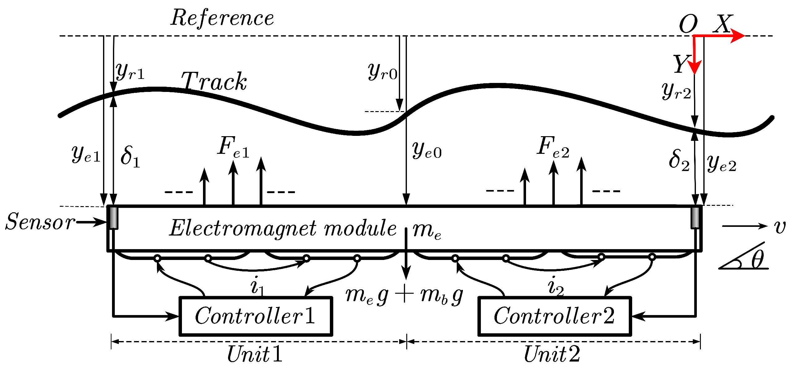
2.1. Modeling of the Electromagnetic Levitation System

As the module levitation systems in the maglev train are decoupled with each other, we take a single module levitation system as the typical analysis object, which can fully reflect the vertical dynamic difference of the levitation system. Therefore, the vertical dynamic model, including a rigid track and a rigid electromagnet module, is established, which is shown in Figure 1. The electromagnet module moves at a constant speed v to the right, which is the positive direction of the X-axis. The origin O of the coordinate system of the electromagnet corresponds to the right terminal of the electromagnet. There are two degrees of freedom of the electromagnetic module: vertical movement in the Y-axis and rotation around the center of the mass. Variable $\theta$ is the rotation angle and its positive direction is presented in Figure 1.

In Figure 1, variables $y_r$ and $y_e$ are the vertical displacement in the Y-axis of the track and the electromagnet, respectively. Variables ${\delta }_1$ and ${\delta }_2$ are the levitation gaps measured by the two gap-sensors, which are configured at the two terminals of the electromagnet module. There are four coils in an electromagnet module, which are connected by series and divided into two units controlled by two voltage-chopping controllers, separately. Each controller uses the measured levitation gap $\delta$ to control the coil current i, thus achieving stable levitation gap control. Variables $F_{e1}$ and $F_{e2}$ are the electromagnetic attraction forces produced by the electrified electromagnet and the magnetic track, which are evenly distributed along the pole face. Variable $m_e$ is the equivalent mass of the electromagnet module, and $m_b$ is the equivalent mass of the vehicle body transmitted through air-springs.

According to Figure 1, the vertical displacements of $y_{r0}$ and $y_{r1}$ are deduced by $y_{r2}$:

$$y_{r0}\left(t\right)=y_{r2}\left(t-2l/v\right)$$

(1)

$$y_{r1}\left(t\right)=y_{r2}\left(t-4l/v\right)$$

(2)

where l is the length of a single coil.

The measured levitation gaps ${\delta }_1\left(t\right)$ and ${\delta }_2\left(t\right)$ are:

$${\delta }_1\left(t\right)=y_{e1}\left(t\right)-y_{r2}\left(t-4l/v\right)$$

(3)

$${\delta }_2\left(t\right)=y_{e2}\left(t\right)-y_{r2}\left(t\right)$$

(4)

The average gaps ${\tilde{\delta }}_1$ and ${\tilde{\delta }}_2$ are the mean value of the gap integration along the pole surface of the electromagnet:

$${\tilde{\delta }}_1\left(t\right)=\frac{3}{4}{y}_{e1}\left(t\right)+\frac{1}{4}{y}_{e2}\left(t\right)-\frac{v}{2l}{\int }_{-4l/v}^{-2l/v}{f}_r\left(t+\tau \right)d\tau$$

(5)

$${\tilde{\delta }}_2\left(t\right)=\frac{1}{4}{y}_{e1}\left(t\right)+\frac{3}{4}{y}_{e2}\left(t\right)-\frac{v}{2l}{\int }_{-2l/v}^0{f}_r\left(t+\tau \right)d\tau$$

(6)

The relationship between controlled voltage $u\left(t\right)$ and current $i\left(t\right)$ for each single coil of two units are as follows:

$$\frac{u_1\left(t\right)}{2}=R{i}_1\left(t\right)+\frac{u_0{N}^{2}A}{2{\tilde{\delta }}_1\left(t\right)}{\dot{i}}_1\left(t\right)-\frac{u_0{N}^{2}A{i}_1\left(t\right)}{2{\tilde{\delta }}_1^2\left(t\right)}{\dot{\tilde{\delta }}}_1\left(t\right)$$

(7)

$$\frac{u_2\left(t\right)}{2}=R{i}_2\left(t\right)+\frac{u_0{N}^{2}A}{2{\tilde{\delta }}_2\left(t\right)}{\dot{i}}_2\left(t\right)-\frac{u_0{N}^{2}A{i}_2\left(t\right)}{2{\tilde{\delta }}_2^2\left(t\right)}{\dot{\tilde{\delta }}}_2\left(t\right)$$

(8)

where R is the resistance of a single-coil, N is the turn number of a single-coil, A is the pole area corresponding to the length of a single-coil, and $u_0$ is the magnetic permeability of a vacuum.

If the magnetic leakage and the magnetic resistance of the track and electromagnet are ignored, the average electromagnetic forces provided by each two coils can be expressed as follows:

$$F_{e1}\left(t\right)=\frac{u_0{N}^{2}A}{2}\frac{i_1^2\left(t\right)}{{\tilde{\delta }}_1^2\left(t\right)}$$

(9)

$$F_{e2}\left(t\right)=\frac{u_0{N}^{2}A}{2}\frac{i_2^2\left(t\right)}{{\tilde{\delta }}_2^2\left(t\right)}$$

(10)

The vertical movement equation can be expressed as:

$$m_e{\ddot{y}}_{e0}\left(t\right)=\left(m_e+m_b\right)g-\left(F_{e1}\left(t\right)+F_{e2}\left(t\right)\right)$$

(11)

where g is the acceleration of gravity.

The rotation equation is:

$$I_e\ddot{\theta }\left(t\right)=\left(F_{e2}\left(t\right)-F_{e1}\left(t\right)\right)l$$

(12)

where $I_e=4m_e{l}^2/3$ is the inertia moment of the electromagnet module.

As the parameters of two units are just the same, according to Equations (9)–(11), the equilibrium current $i_0$ at the desired levitation gap ${\delta }_0$ is expressed by:

$$i_0=\frac{{\delta }_0}{N}\sqrt{\frac{\left(m_e+m_b\right)g}{u_{0}A}}$$

(13)

As the electromagnetic force is inversely proportional to the square of the levitation gap, the levitation system is inherently unstable. Researchers have carried out a wide range of researches [25,26,27,28,29] to achieve stable levitation control. However, state feedback control [30] is the typical levitation control algorithm. Here, the levitation gap signal, inertial velocity signal, and inertial acceleration signal are used to form a PIDA (Proportional-Integral-Derivative-Acceleration) control algorithm. Li [31] introduced the cascade control into the levitation control, which is adopted in this paper. The current inner-loop uses proportional control to speed up the current response and overcome the time delay caused by inductance.

The PIDA-type desired currents $i_{e1}\left(t\right)$ and $i_{e2}\left(t\right)$ are:

$$\begin{array}{cc}\hfill i_{e1}\left(t\right)=& k_P\left({\delta }_1\left(t\right)-{\delta }_0\right)+k_I{\int }_0^t\left({\delta }_1\left(t\right)-{\delta }_0\right)dt\hfill \\ \hfill & +k_D{\dot{y}}_{e1}\left(t\right)+k_A{\ddot{y}}_{e1}\left(t\right)+i_0\hfill \end{array}$$

(14)

$$\begin{array}{cc}\hfill i_{e2}\left(t\right)=& k_P\left({\delta }_2\left(t\right)-{\delta }_0\right)+k_I{\int }_0^t\left({\delta }_2\left(t\right)-{\delta }_0\right)dt\hfill \\ \hfill & +k_D{\dot{y}}_{e2}\left(t\right)+k_A{\ddot{y}}_{e2}\left(t\right)+i_0\hfill \end{array}$$

(15)

where $k_P$, $k_I$, $k_D$, and $k_A$ are the feedback parameters.

The controlled voltages $u_1\left(t\right)$ and $u_2\left(t\right)$ are deduced by:

$$u_1\left(t\right)=k_c\left(i_{e1}\left(t\right)-i_1\left(t\right)\right)$$

(16)

$$u_2\left(t\right)=k_c\left(i_{e2}\left(t\right)-i_2\left(t\right)\right)$$

(17)

where $k_c$ is the current loop gain.

The motion of the levitation system is determined by Equations (1)–(17). Here, the vertical dynamic model of the electromagnetic levitation system is built.

2.2. Linear Model in the Frequency Domain

Under the levitation control, the levitation electromagnet module strictly tracks the space trajectory of the track, but in this process, the levitation gaps fluctuate around the set gap ${\delta }_0$. The linear model can be used to simplify the analysis process without introducing obvious errors. By using the Laplace transform function, the linear model is changed into the frequency domain.

Define $k_{u1}\left(s\right)=e^{-\frac{4ls}{v}}$, $k_{u2}\left(s\right)=\frac{v}{2ls}\left(e^{-\frac{2ls}{v}}-e^{-\frac{4ls}{v}}\right)$, and $k_{u3}\left(s\right)=\frac{v}{2ls}\left(1-e^{-\frac{2ls}{v}}\right)$, then the levitation gap and average gap equations in the frequency domain are:

$${\delta }_1\left(s\right)=y_{e1}\left(s\right)-k_{u1}{y}_{r2}\left(s\right)$$

(18)

$${\delta }_2\left(s\right)=y_{e2}\left(s\right)-y_{r2}\left(s\right)$$

(19)

$${\tilde{\delta }}_1\left(s\right)=\frac{3}{4}{y}_{e1}\left(s\right)+\frac{1}{4}{y}_{e2}\left(s\right)-k_{u2}{y}_{r2}\left(s\right)$$

(20)

$${\tilde{\delta }}_2\left(s\right)=\frac{1}{4}{y}_{e1}\left(s\right)+\frac{3}{4}{y}_{e2}\left(s\right)-k_{u3}{y}_{r2}\left(s\right)$$

(21)

Define $k_i=0.5u_0{N}^{2}A{i}_0{\delta }_0^{-2}$, $k_z=0.5u_0{N}^{2}A{i}_0^2{\delta }_0^{-3}$, $L_0=0.5u_0{N}^{2}A{\delta }_0^{-1}$, then the current equations are:

$$\begin{array}{cc}\hfill {\dot{i}}_1\left(s\right)=& \frac{k_c{k}_P+k_c{k}_I\frac{1}{s}}{2L_0}{\delta }_1\left(s\right)+\frac{k_c{k}_D}{2L_0}{\dot{y}}_{e1}\left(s\right)+\frac{k_c{k}_A}{2L_0}{\ddot{y}}_{e1}\left(s\right)\hfill \\ \hfill & -\frac{2R+k_c}{2L_0}{i}_1\left(s\right)+\frac{k_i}{L_0}{\dot{\tilde{\delta }}}_1\left(s\right)\hfill \end{array}$$

(22)

$$\begin{array}{cc}\hfill {\dot{i}}_2\left(s\right)=& \frac{k_c{k}_P+k_c{k}_I\frac{1}{s}}{2L_0}{\delta }_2\left(s\right)+\frac{k_c{k}_D}{2L_0}{\dot{y}}_{e2}\left(s\right)+\frac{k_c{k}_A}{2L_0}{\ddot{y}}_{e2}\left(s\right)\hfill \\ \hfill & -\frac{2R+k_c}{2L_0}{i}_2\left(s\right)+\frac{k_i}{L_0}{\dot{\tilde{\delta }}}_2\left(s\right)\hfill \end{array}$$

(23)

According to Equations (11) and (12), the kinetic equations are as follows:

$${\ddot{y}}_{e1}\left(s\right)=-\frac{5k_i}{m_e}{i}_1\left(s\right)+\frac{k_i}{m_e}{i}_2\left(s\right)+\frac{5k_z}{m_e}{\tilde{\delta }}_1\left(s\right)-\frac{k_z}{m_e}{\tilde{\delta }}_2\left(s\right)$$

(24)

$${\ddot{y}}_{e2}\left(s\right)=-\frac{5k_i}{m_e}{i}_2\left(s\right)+\frac{k_i}{m_e}{i}_1\left(s\right)+\frac{5k_z}{m_e}{\tilde{\delta }}_2\left(s\right)-\frac{k_z}{m_e}{\tilde{\delta }}_1\left(s\right)$$

(25)

Let $X={\left[\begin{array}{cccccc}{y}_{e1}& {\dot{y}}_{e1}& y_{e2}& {\dot{y}}_{e2}& i_1& i_2\end{array}\right]}^T$, $u=y_{r2}\left(s\right)$, and $Y={\left[\begin{array}{cc}{\delta }_1& {\delta }_2\end{array}\right]}^T$, the Equations (18)–(25) are transferred into a state-space equation as follows:

$$\left\{\begin{array}{c}\dot{X}=A_{s}X+B_{s}u\hfill \\ Y=C_{s}X+D_{s}u\hfill \end{array}\right.$$

(26)

where:

$$A_s=\left[\begin{array}{cccccc}0& 1& 0& 0& 0& 0\\ a_{21}& 0& a_{23}& 0& a_{25}& a_{26}\\ 0& 0& 0& 1& 0& 0\\ a_{23}& 0& a_{21}& 0& a_{26}& a_{25}\\ a_{51}& a_{52}& a_{53}& a_{54}& a_{55}& a_{56}\\ a_{53}& a_{54}& a_{51}& a_{52}& a_{56}& a_{55}\end{array}\right]$$

(27)

$$B_s={\left[\begin{array}{cccccc}0& b_2& 0& b_4& b_5& b_6\end{array}\right]}^T$$

(28)

$$C_s=\left[\begin{array}{cccccc}1& 0& 0& 0& 0& 0\\ 0& 0& 1& 0& 0& 0\end{array}\right]$$

(29)

$$D_s={\left[\begin{array}{cc}-k_{u1}& -1\end{array}\right]}^T$$

(30)

$$\left\{\begin{array}{c}{a}_{21}=3.5k_z{m}_e^{-1}\hfill \\ a_{23}=0.5k_z{m}_e^{-1}\hfill \\ a_{25}=-5k_i{m}_e^{-1}\hfill \\ a_{26}=k_i{m}_e^{-1}\hfill \\ a_{51}=\left(k_c{k}_P+k_c{k}_I{s}^{-1}+3.5k_z{k}_c{k}_A{m}_e^{-1}\right)2^{-1}{L}_0^{-1}{s}^{-1}\hfill \\ a_{52}=0.5k_c{k}_D{L}_0^{-1}+0.75k_i{L}_0^{-1}\hfill \\ a_{53}=0.25k_z{k}_c{k}_A{m}_e^{-1}{L}_0^{-1}\hfill \\ a_{54}=0.25k_i{L}_0^{-1}\hfill \\ a_{55}=-R{L}_0^{-1}-0.5k_c{L}_0^{-1}-2.5k_c{k}_A{k}_i{m}_e^{-1}{L}_0^{-1}\hfill \\ a_{56}=0.5k_c{k}_A{k}_i{m}_e^{-1}{L}_0^{-1}\hfill \end{array}\right.$$

(31)

$$\left\{\begin{array}{c}{b}_2=\left(-5k_{u2}+k_{u3}\right)k_z{m}_e^{-1}\hfill \\ b_4=\left(-5k_{u3}+k_{u2}\right)k_z{m}_e^{-1}\hfill \\ b_5=-\frac{\left(k_c{k}_P+k_c{k}_I{s}^{-1}\right)k_{u1}+k_c{k}_A{k}_z{m}_e^{-1}\left(5k_{u2}-k_{u3}\right)+2k_i{k}_{u2}s}{2L_0}\hfill \\ b_6=-\frac{\left(k_c{k}_P+k_c{k}_I{s}^{-1}\right)+k_c{k}_A{k}_z{m}_e^{-1}\left(5k_{u3}-k_{u2}\right)+2k_i{k}_{u3}s}{2L_0}\hfill \end{array}\right.$$

(32)

The transfer functions from $u\left(s\right)$ to $Y\left(s\right)$:

$$G_s\left(s\right)=C_s{\left(s{I}_{6\times 6}-A_s\right)}^{-1}{B}_s+D_s$$

(33)

Then, the dynamic response of the levitation gap is:

$$Y\left(s\right)=G_s\left(s\right)u\left(s\right)$$

(34)

The track irregularity is generally considered as a stationary random process [4], which is generally analyzed by a PSD function. For each frequency in the PSD function, there is no phase correlation with other frequencies, so the discrete frequency analysis method can be used to analyze each frequency separately. Under the excitation of the track irregularity, the levitation gap signal is also a stationary random signal. Therefore, the variance of the time-domain levitation gap signal can be obtained by the spectral integration of the PSD functions according to Parseval’s theorem. To simplify the analysis, we transform the PSD function into the amplitude spectrum function as the main function.

The space trajectory of the track in a constant wavelength $\lambda$ at a constant speed v is modeled as a sinusoid function:

$$y_{r2}\left(t\right)=A_{r}sin\left(wt\right)+A_{r0}$$

(35)

where $w=2\pi v/\lambda$, $A_r$ is the amplitude of the track, and $A_{r0}$ is the constant value. To simplify the analysis, we set $A_{r0}=0$. Then, the output levitation gaps are deduced as:

$$Y\left(t\right)=A_r\left|G_s\left(s=jw\right)\right|sin\left(wt+\angle G_s\left(s=jw\right)\right)$$

(36)

Therefore, the amplitude of levitation gaps are deduced as:

$$\left|\delta \left(s=jw\right)\right|=A_r\left|G_s\left(s=jw\right)\right|$$

(37)

The amplitude of the levitation gap is composed of two parts, the amplitude of the track $A_r$ and the amplitude of transfer function $\left|G_s\right|$. To simulate the real track situation, we choose the German low interference track PSD function as the input source in this paper. The PSD function $S_v\left(\Omega \right)$ is:

$$S_v\left(\Omega \right)=\frac{A_v{\Omega }_c^2}{\left({\Omega }^2+{\Omega }_r^2\right)\left({\Omega }^2+{\Omega }_c^2\right)}$$

(38)

where $\Omega =2\pi {\lambda }^{-1}$, $A_v=4.032\times {10}^{-7}{\mathrm{m}}^2·\mathrm{rad}/\mathrm{m}$, ${\Omega }_c=0.8246\mathrm{rad}/\mathrm{m}$, and ${\Omega }_r=0.0206\mathrm{rad}/\mathrm{m}$.

The track amplitude $A_r\left(\lambda \right)$ is deduced from $S_v\left(\lambda \right)$:

$$A_r\left(\lambda \right)=k_r\sqrt{S_v\left(\lambda \right)}$$

(39)

According to practical experience, we set $k_r=0.0247$.

3. Vertical Dynamic Prediction under Track Irregularity

The characteristic equations of transfer function $G_s$ is:

$$\begin{array}{cc}\hfill \Delta \left(s\right)=& \left(2L_0{m}_e\right)s^4+\left(\left(2R+k_c\right)m_e+5k_c{k}_A{k}_i\right)s^3\hfill \\ \hfill & +\left(5k_c{k}_D{k}_i+3.5k_i^2\right)s^2+\left(5k_c{k}_P{k}_i-3.5k_z\right)s\hfill \\ \hfill & +\left(5k_c{k}_I{k}_i\right)\hfill \end{array}$$

(40)

We select parameters according to the actual parameters of the low-speed maglev train: $m_e=1000$ kg, $m_b=1300$ kg, $N=360$, $R=0.55$ $\Omega$, $A=0.0185$ m${}^2$, $l=0.66$ m, $u_0=4\pi \times {10}^{-7}$. The control parameters are: $k_p=4000$, $k_D=80$, $k_I=20,000$, $k_a=0.2$, and $k_c=110$. Obviously, the parameters above satisfy the Routh criterion of Equation (40), which means the levitation system is stable.

As the dynamic model is affected by the track wavelength $\lambda$ and the vehicle speed v at the same time, to depict this influence, we have drawn a 3-D graph related to $\lambda$ and v. The 3-D amplitude spectrums of the levitation gaps are shown in Figure 2.

According to Figure 2, the following conclusions can be drawn:

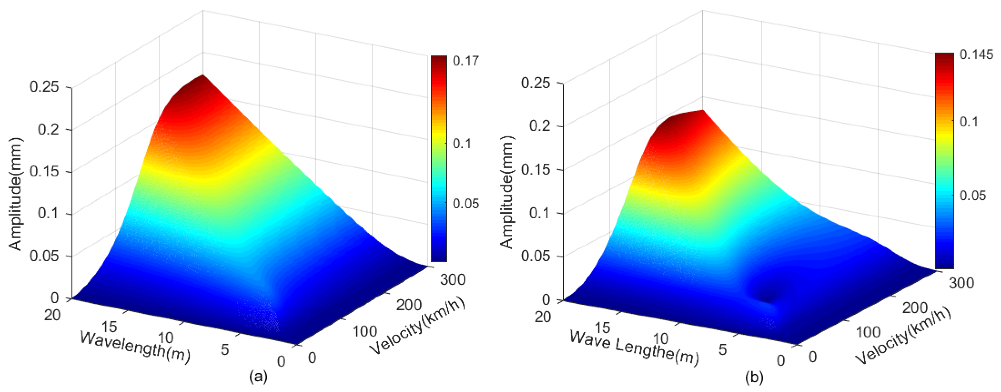
• When the speed is very low, the amplitudes of both levitation gaps are relatively small at different wavelengths, which means that the electromagnet module can strictly track the space trajectory of the track. With the increase of the speed, the amplitude spectrum values of the levitation gaps generally rise, which means that the tracking performance of the electromagnet module is reduced.
• When the wavelength is close to 0, the amplitude spectrum values of both levitation gaps are relatively small at different speeds. In this case, the electromagnet module keeps its inertial position stable and does not track the space trajectory of the track. Therefore, the amplitude of the levitation gap is equal to the amplitude of the track. However, as the amplitude of the track at small wavelengths is small, the amplitude values of the levitation gaps are relatively small. Although this means that the tracking performance of the levitation control system is very weak, it is consistent with the phenomenon that the high-frequency signal is ignored, which is expected in the levitation control system.
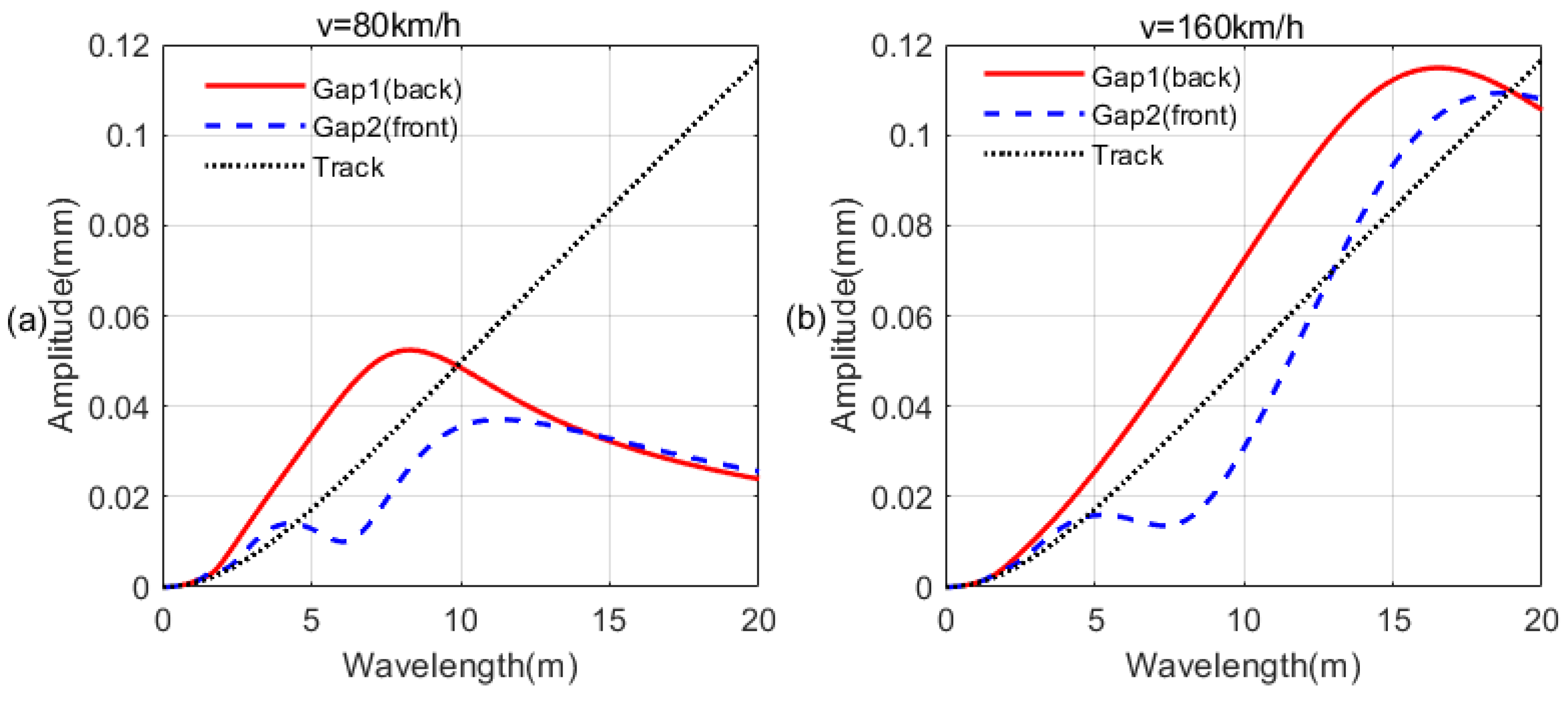
• The maximum value appears in the case of high speed and large wavelength, which is consistent with engineering experience. When the speed is very high, we need to pay special attention to the track irregularities at large wavelengths. Due to the larger amplitude of the long-wave track irregularities, the contributions of the long-wave track irregularities to the gap deviation is also large.
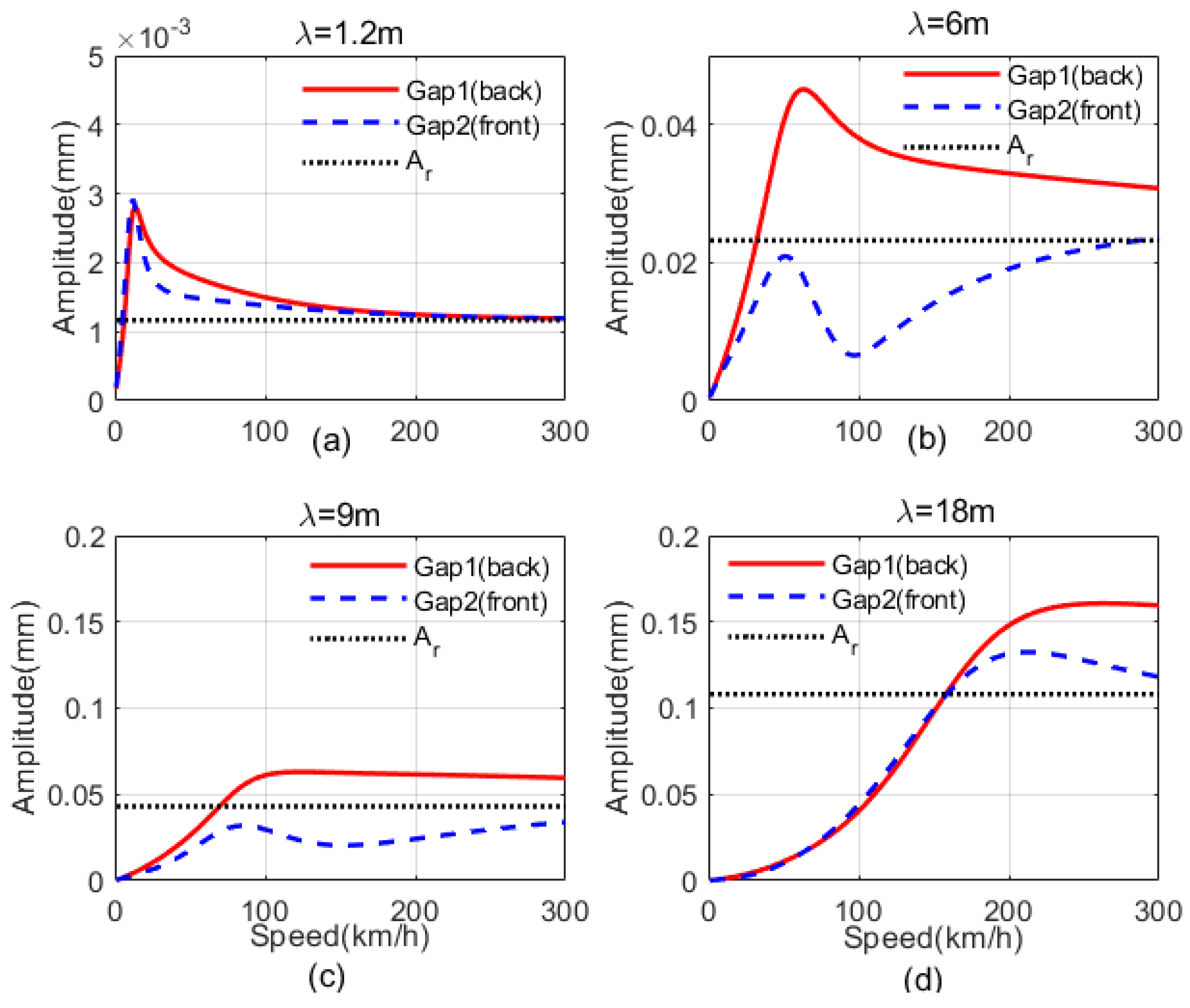
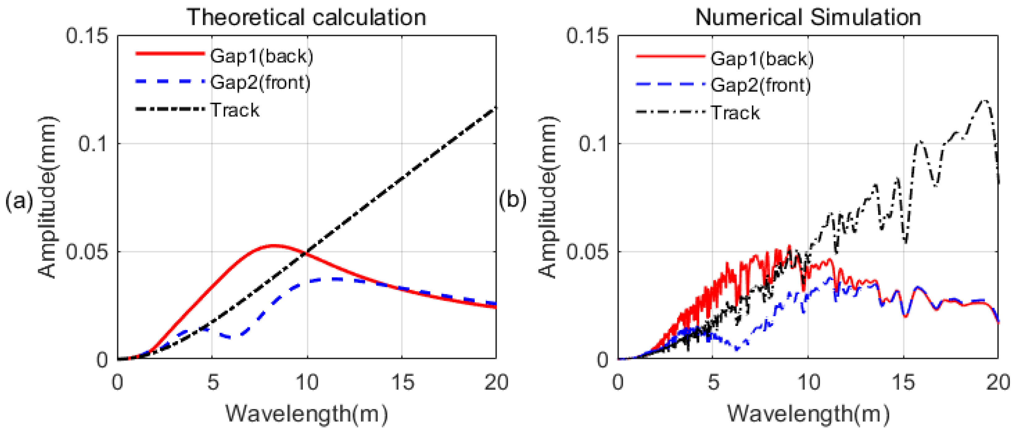
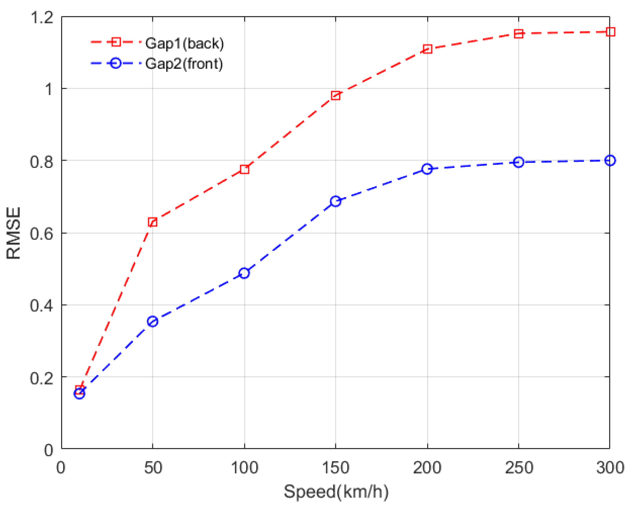
• The amplitudes of the two levitation gaps are different. Moreover, in a broad range of wavelength and speed, the amplitudes of the back gap are larger than that of the front gap. As the input amplitudes of the two levitation gaps are the same, the difference in the transfer functions is the main reason for the dynamic response difference.

3.1. Analysis of Levitation Gap Deviation

According to the Parseval’s theorem, the area of amplitude spectrum function reflects the variance of the random signal in the time-domain. The amplitude spectrum area of levitation gaps is shown in Figure 3.

According to Figure 3, it is found that the amplitude spectrum areas of both levitation gaps generally increase with the increase of vehicle speed, which is consistent with the practical experience. Due to the fact that the wavelengths greater than 20 m are not considered, the amplitude spectrum areas of both levitation gaps tend to be stable when the speed is greater than 200 km/h. At the same time, the amplitude spectrum area of the back levitation gap is greater than that of the front levitation gap at all speeds, which is consistent with the conclusions drawn from Figure 2.

As the amplitude spectrum area increases with speed, it means that the deviation degree of the levitation gap signal increase with speed too. However, the deviation range of the levitation gap signal is limited, and the safe range is ±4 mm. Therefore, the stability of the levitation system is challenged with the increase of the vehicle speed. With the general speed-up of the urban maglev system, it is necessary to find ways to decrease the deviation of the levitation gap at high speed.

3.2. Analysis of Typical Wavelengths

There are typical periodical track irregularities in the maglev track, which are related to the sleeper pace, F-rail section, and rail beam span. Here, we select typical wavelengths: 1.2 m (sleeper pace), 6 m (F-rail section), 9 m (half-track beam span), and 18 m (typical simple-elevated track beam span). The amplitude spectrums of levitation gaps related to vehicle speed at different wavelengths are shown in Figure 4. The amplitudes of the periodical track irregularities $A_r$ at different wavelengths are shown in Figure 4 too, which provide a reference to the amplitude spectrums of levitation gaps.

According to Figure 4, for the short-wave wavelength of 1.2 m (sleeper pace), the maximum points of the two levitation gaps appear at 13 km/h (the back gap) and 12 km/h (the front gap), respectively. When the speed is lower than 13 km/h, the amplitudes of the front levitation gap are larger than that of the back levitation gap, which is different from the general trend. With the increase of speed, the amplitudes of the two levitation gaps tend to be equal to the track input amplitude at high speed.

For the wavelength of 6 m (F-rail section), the maximum point of the back levitation gaps appears at 63 km/h. In general, the amplitudes of the back levitation gap increase first and then decrease, while the amplitudes of the front levitation gap experience twice the increase, with a local minimum point at around 100 km/h.

For the wavelength of 9 m (half-track beam span), the maximum point of the back levitation gap appears at 124 km/h. The amplitudes of the front levitation gap also experience twice the increase, with a local minimum point at around 150 km/h.

For the wavelength of 18 m (typical simple-elevated track beam span), the maximum points of the two levitation gaps appear at 263 km/h (the back gap) and 213 km/h (the front gap), respectively. In a certain speed range, the amplitude of the front levitation gap is larger than that of the back levitation gap. The tracking performance is strong when the amplitude of the levitation gap is less than the input amplitude of the track. Therefore, the electromagnet module has a good tracking ability for the wavelength of 18 m when the speed is less than 158 km/h.

In general, the two levitation units have different amplitude responses at different wavelengths, which need to be analyzed specifically. The general trend is that at low speed, the amplitude response is smaller than the track input, and the tracking ability is strong. At high speed, the tracking ability is weak, and the amplitude response is even larger than the track input amplitude. Then with the continuous increase of speed, the amplitude response is equal to the track input amplitude. This phenomenon is consistent with the characteristic that the electromagnetic levitation system tracks the low-frequency signal and ignores the high-frequency signal. From the previous analysis, it can be concluded that the levitation system has good tracking performance for a track profile change below 2 Hz.

3.3. Analysis of Typical Speeds

We select 80 and 160 km/h as typical speed values for analysis, and its amplitude spectrums are shown in Figure 5. The track amplitudes $A_r\left(\lambda \right)$ are labeled as “Track” in Figure 5. According to Figure 5, the amplitudes of the track irregularities generally rise with the wavelengths, which means that the longer wavelength track irregularities have larger amplitudes.

According to Figure 5, when the speed is 80 km/h, the maximum amplitude response values of the two levitation gap appear at the wavelength of 8.3 and 11.3 m, respectively. The amplitude response of the front levitation gap is smaller than that of the track in a wide range of wavelengths, and the amplitude response of the back levitation gap is larger than that of the track in a certain range of wavelengths. The back levitation unit has a good tracking ability for the track input when the wavelength is greater than 9.88 m.

When the speed is 160 km/h, the maximum values of the two levitation gap appear at the wavelength of 16.5 and 18.6 m, respectively. The two levitation units have good tracking ability for the track input when the wavelength is greater than 19 m.

From the analysis above, it can be concluded that with the increase of the speed, the wavelength range that the levitation units have strong tracking ability decreases. However, due to the larger track amplitude of the longer wavelength irregularity, the maximum points of the amplitude spectrums of both levitation units are larger with the increase of the speed, which leads to the rise of the amplitude spectrum area.

4. Numerical Simulation

We have carried out numerical simulations to verify the correctness of the theoretical analysis. By using the IFFT method, the track irregularity data obtained from the low interference German PSD function is shown in Figure 6. The spacial step of the data is 0.25 m, and the total length is 3.276 km. The maximum value is 3.02 mm, and the minimum value is −2.93 mm. The PSD diagram of simulation data and the low interference German PSD function are shown in Figure 7. As shown in Figure 7, the PSD value of the simulation data is basically the same as that of the German track within the set wavelength range of 0.05–20 m, which shows that the IFFT method is successful.

In the MATLAB environment, we established the dynamic model of the electromagnetic levitation system based on Equations (1)–(17), and use the numerical integration method to solve the differential equations. In the numerical simulation, the time step is 0.5 ms and the total simulation time is 147 s. We set the vehicle speed as 80 km/h. The two levitation gap signals in numerical simulation at 80 km/h are shown in Figure 8, and the amplitude spectrums of the levitation gap signals are shown in Figure 9b. Figure 9a demonstrates the theoretical calculation results at 80 km/h.

The root mean square error (RMSE) function is adopted to measure the deviation degree of time-domain signal, which has the property of variance and the physical signal unit at the same time. The RMSE is defined as:

$$\mathrm{RMSE}=\sqrt{\frac{1}{n}\sum _{i=1}^n{\left({\delta }_i-{\delta }_0\right)}^2}$$

(41)

Here, ${\delta }_0=9$ mm in Figure 8.

According to Figure 8, the RMSE value of the back levitation gap is 74.2% larger than that of the front levitation gap. At the same time, the deviation range of the two levitation gaps are $\left[-2.547,2.256\right]$ mm (the back), and $\left[-1.541,1.364\right]$ mm (the front), respectively. These are consistent with the previous analysis result in Section 3.1 that the deviation degree of the back levitation gap is larger than that of the front levitation gap.

According to Figure 9, the amplitude spectrums of the numerical simulation signals are highly approximate to the theoretical analysis results, which verifies the correctness of the theoretical analysis method. Due to the error of the IFFT method, there are local fluctuations in the amplitude spectrums in Figure 9.

The RMSE values of levitation gap errors at different speeds in the numerical simulation are shown in Figure 10. The maximum values of levitation gap errors at different speeds are shown in Figure 11.

According to Figure 10, it is found that the RMSE values of both levitation gap errors generally increase with the increase of vehicle speed and tend to be stable when the speed is greater than 200 km/h. The maximum value of the levitation gap error in Figure 11 has the same trend with the RMSE value. At the same time, it is found that these trends are consistent with that of the amplitude spectrum area in Figure 3, which means that the amplitude spectrum area in the theoretical calculation is the key indicator to present the deviation degree of the levitation gap signals.

According to Figure 11, under the excitation of the german low interference track irregularity, the maximum value of the levitation gap error may exceed the safe range when the speed is larger than 250 km/h. The actual track irregularity condition may be worse than that of the low interference track. Due to the fact that the strength of the urban maglev track is weaker than that of the high-speed maglev track and the simple-supported beam is often used, the corresponding wavelength amplitude of the simple-supported beam is relatively large, which means the actual levitation system may exceed the safe range when the speed is smaller than 250 km/h.

5. Conclusions

Due to the limited deviation range of the levitation gap, the vehicle/track coupling problem in the urban maglev system is prominent. With the further development and speed-up of the world’s urban maglev systems, the vertical dynamic response of the levitation system under the track irregularity needs to be further studied. In this paper, a vertical dynamic model, including the electromagnet module and the track, is established. The amplitude spectrum of the levitation gap is obtained by using the discrete frequency analysis method, which can fully reflect the vertical dynamic response of the electromagnetic levitation system. The theoretical analysis shows that the model can be used to predict the dynamic response of the levitation system, including the dynamic response difference between the two levitation gaps and the problem that the levitation gap exceeds the safe range at high speed. The analysis method provides a reference for the levitation controller design for the maglev train, which is helpful to improve the stability of the electromagnetic levitation systems and ride comfort of the maglev train.

References

1. Lee, H.W.; Lee, J.; Kim, K.C. Review of Maglev Train Technologies. IEEE Trans. Magn. 2006, 42, 1917–1925. [Google Scholar]
2. Yan, L. Progress of the Maglev Transportation in China. IEEE Trans. Appl. Supercond. 2006, 16, 1138–1141. [Google Scholar]
3. Lin, G.; Sheng, X. Application and further development of Maglev transportation in China. Transp. Syst. Technol. 2018, 4, 36–43. [Google Scholar] [CrossRef]
4. Zhang, G.; Li, J.; Yang, Z. Estimation of Power Spectrum Density Track Irregularities of Low-speed maglev railway lines. J. China Railw. Soc. 2011, 33, 73–78. [Google Scholar]
5. Zhou, D.; Yu, P.; Li, J.; Wang, L. An adaptive vibration control method to suppress the vibration of the maglev train caused by track irregularities. J. Sound Vib. 2017, 408, 331–350. [Google Scholar] [CrossRef]
6. Shu, G.; Meisinger, R.; Shen, G. Simulation of a maglev train with periodic guideway deflections. In Proceedings of the 2008 Asia Simulation Conference—7th International Conference on System Simulation and Scientific Computing, Beijing, China, 10–12 October 2008; pp. 421–425. [Google Scholar]
7. Yu, P.; Li, J.; Li, J.; Wang, L. Influence of track periodical irregularities to the suspension system of low-speed maglev vehicle. In Proceedings of the 2015 34th Chinese Control Conference (CCC), Hangzhou, China, 28–30 July 2015; pp. 8479–8484. [Google Scholar]
8. Wang, Z.; Long, Z.; Li, X. Track Irregularity Disturbance Rejection for Maglev Train Based on Online Optimization of PnP Control Architecture. IEEE Access 2019, 7, 12610–12619. [Google Scholar] [CrossRef]
9. Yau, J.D. Vibration control of maglev vehicles traveling over a flexible guideway. J. Sound Vib. 2009, 321, 184–200. [Google Scholar] [CrossRef]
10. Ren, S.; Arie, R.; Klap, K. Dynamic Simulation of the Maglev Vehicle/Guideway System. J. Bridge Eng. 2009, 15, 269–278. [Google Scholar] [CrossRef]
11. Shi, J.; Wei, Q.; Zhao, Y. Analysis of dynamic response of the high-speed EMS maglev vehicle/guideway coupling system with random irregularity. Vehicle Syst. Dyn. 2007, 45, 1077–1095. [Google Scholar] [CrossRef]
12. Zhao, C.; Zhai, W. Maglev Vehicle/Guideway Vertical Random Response and Ride Quality. Veh. Syst. Dyn. 2002, 38, 185–210. [Google Scholar] [CrossRef]
13. Lee, J.S.; Kwon, S.D.; Kim, M.Y.; Yeo, I.H. A parametric study on the dynamics of urban transit maglev vehicle running on flexible guideway bridges. J. Sound Vib. 2009, 328, 301–317. [Google Scholar] [CrossRef]
14. Wang, Z.L.; Xu, Y.L.; Li, G.Q.; Yang, Y.B.; Chen, S.W.; Zhang, X.L. Modelling and validation of coupled high-speed maglev train-and-viaduct systems considering support flexibility. Vehicle Syst. Dyn. 2019, 57, 161–191. [Google Scholar] [CrossRef]
15. Zhou, D.; Hansen, C.H.; Li, J. Suppression of maglev vehicle–girder self-excited vibration using a virtual tuned mass damper. J. Sound Vib. 2011, 330, 883–901. [Google Scholar] [CrossRef]
16. Li, J.; Li, J.; Zhou, D.; Cui, P.; Yu, P. The Active Control of Maglev Stationary Self-Excited Vibration With a Virtual Energy Harvester. IEEE Trans. Ind. Electron. 2015, 62, 2942–2951. [Google Scholar] [CrossRef]
17. Min, D.J.; Kwon, S.D.; Kwark, J.W.; Kim, M.Y. Gust Wind Effects on Stability and Ride Quality of Actively Controlled Maglev Guideway Systems. Shock Vib. 2017, 2017, 1–23. [Google Scholar] [CrossRef]
18. Shi, J.; Wang, Y. Dynamic response analysis of single-span guideway caused by high speed maglev train. Lat. Am. J. Solid. Stuc. 2011, 8, 213–228. [Google Scholar] [CrossRef] [Green Version]
19. Han, H.S.; Yim, B.H.; Lee, N.J.; Kim, Y.J. Prediction of ride quality of a Maglev vehicle using a full vehicle multi-body dynamic model. Veh. Syst. Dyn. 2009, 47, 1271–1286. [Google Scholar] [CrossRef]
20. Huang, J.; Zhou, X.; Shang, L.; Wu, Z.; Xu, W. Influence analysis of track irregularity on running comfort of Maglev train. Transp. Syst. Technol. 2018, 4, 129–140. [Google Scholar] [CrossRef]
21. Li, Y.; Yu, P.; Zhou, D.; Li, J. Magnetic flux feedback strategy to suppress the gap fluctuation of Low speed maglev train caused by track steps. In Proceedings of the 2018 37th Chinese Control Conference (CCC), Wuhan, China, 25–27 July 2018; pp. 983–989. [Google Scholar]
22. Leng, P.; Li, Y.; Zhou, D.; Li, J.; Zhou, S. Decoupling Control of Maglev Train Based on Feedback Linearization. IEEE Access 2019, 7, 130352–130362. [Google Scholar] [CrossRef]
23. Zhou, D.; Yu, P.; Li, J.; Wang, L. An Approach to Reduce Vibration of the Levitation System when the Urban Maglev Train is Traveling. In Proceedings of the 2018 37th Chinese Control Conference (CCC), Wuhan, China, 25–27 July 2018; pp. 7736–7741. [Google Scholar]
24. Li, Y.; Zhou, D.; Cui, P.; Yu, P.; Chen, Q.; Wang, L.; Li, J. Dynamic Performance Optimization of Electromagnetic Levitation System Considering Sensor Position. IEEE Access 2020, 8, 29446–29455. [Google Scholar] [CrossRef]
25. Li, J.; Li, J.; Zhang, G. A practical robust nonlinear controller for maglev levitation system. J. Cent. South. Univ. 2013, 20, 2991–3001. [Google Scholar] [CrossRef]
26. Pan, Y.; Wang, J. Model Predictive Control of Unknown Nonlinear Dynamical Systems Based on Recurrent Neural Networks. IEEE Trans. Ind. Electron. 2012, 59, 3089–3101. [Google Scholar] [CrossRef]
27. Sinha, P.K.; Pechev, A.N. Model reference adaptive control of a maglev system with stable maximum descent criterion. Automatica 1999, 35, 1457–1465. [Google Scholar] [CrossRef]
28. Matsumura, F.; Namerikawa, T.; Hagiwara, K.; Fujita, M. Application of gain scheduled H robust controllers to a magnetic bearing. IEEE Trans. Control Syst. Technol. 1996, 4, 484–493. [Google Scholar] [CrossRef]
29. Chen, Q.; Tan, Y.; Li, J.; Oetomo, D.; Mareels, I. Model-guided data-driven decentralized control for magnetic levitation systems. IEEE Access 2018, 6, 43546–43562. [Google Scholar] [CrossRef]
30. Sinha, P.K. Electromagnetic Suspension Dynamics & Control; Peter Peregrinus Ltd.: London, UK, 1987. [Google Scholar]
31. Li, Y.; Chang, W. Cascade control of an EMS maglev vehicle’s levitation control system. Acta Autom. Sin. 1999, 25, 247–251. [Google Scholar]
Figure 1. Vertical dynamic model of the electromagnet module and the track.
Applsci 10 02580 g001
Figure 2. Amplitude spectrums of levitation gaps. (a) Gap1 (the back), (b) Gap2 (the front).
Applsci 10 02580 g002
Figure 3. Amplitude spectrum area of levitation gaps vs. vehicle speed.
Applsci 10 02580 g003
Figure 4. Amplitude spectrums of levitation gaps vs. vehicle speed. (a) at 1.2 m, (b) at 6 m, (c) at 9 m, (d) at 18 m.
Applsci 10 02580 g004
Figure 5. Amplitude spectrums at different speed vs. track wavelengths. (a) at 80 km/h, (b) at 160 km/h.
Applsci 10 02580 g005
Figure 6. Track irregularity data in numerical simulation.
Applsci 10 02580 g006
Figure 7. Power spectral density (PSD) plot of track irregularity data.
Applsci 10 02580 g007
Figure 8. Levitation gap signals in numerical simulation at 80 km/h. (a) Gap1 (back), (b) Gap2 (front).
Applsci 10 02580 g008
Figure 9. Amplitude spectrums of levitation gap errors at 80 km/h. (a) Theoretical calculation, (b) numerical simulation.
Applsci 10 02580 g009
Figure 10. RMSE values of levitation gap errors vs. vehicle speed.
Applsci 10 02580 g010
Figure 11. Maximum values of levitation gap errors vs. vehicle speed.
Applsci 10 02580 g011