Abstract
Voice signals acquired by a microphone array often include considerable noise and mutual interference, seriously degrading the accuracy and speed of speech separation. Traditional beamforming is simple to implement, but its source interference suppression is not adequate. In contrast, independent component analysis (ICA) can improve separation, but imposes an iterative and time-consuming process to calculate the separation matrix. As a supporting method, principle component analysis (PCA) contributes to reduce the dimension, retrieve fast results, and disregard false sound sources. Considering the sparsity of frequency components in a mixed signal, we propose an adaptive fast speech separation algorithm based on multiple sound source localization as preprocessing to select between beamforming and frequency domain ICA according to different mixing conditions per frequency bin. First, a fast positioning algorithm allows calculating the maximum number of components per frequency bin of a mixed speech signal to prevent the occurrence of false sound sources. Then, PCA reduces the dimension to adaptively adjust the weight of beamforming and ICA for speech separation. Subsequently, the ICA separation matrix is initialized based on the sound source localization to notably reduce the iteration time and mitigate permutation ambiguity. Simulation and experimental results verify the effectiveness and speedup of the proposed algorithm.
1. Introduction
Speech separation aims at the effective extraction of target speech and removal of noise and interference. However, the complexity and variability of voice and speech mixture from different sources undermines the performance of current microphone array-based speech separation as they can retrieve a low separation degree, poor real-time applicability, and inability to adapt to environments. Therefore, adaptive speech separation should be developed with focus on real speech environments.
Beamforming and independent component analysis (ICA) [1,2,3] are the mainstream methods for speech separation. Beamforming processes receive signals from a microphone array to generate a spatially directional beam output pointing towards a single sound source and attenuating sound from other sources [4]. However, simple fixed beamforming has a low performance for speech separation in real environments, and due to the nonorthogonality of the steering vector [5] of each sound source, the interference suppression of adaptive beamforming depends on the accurate estimation of the propagation process [6]. Alterations, such as the use of masks, can improve interference removal, but they can also degrade the target signal components [7]. On the other hand, ICA does not directly utilize the propagation information of sound sources, but it requires the calculation of a separation matrix based on the independence hypothesis. However, multiple iterations for calculating the separation matrix notably increases the computation time [8]. Moreover, ICA requires the number of sound sources to perform reasonable dimensionality reduction in actual use [9]. Therefore, it is usually applied along with principal component analysis (PCA) for dimensionality reduction when there are fewer separated signals than channels and for frequency bins with low signal-to-noise ratio (SNR) [10]. Still, PCA often retrieves a dimension reduction that still exceeds the number of sound sources, and thus several false sound sources are modeled. When using approaches such as the frequency-domain ICA (FDICA), the false sound sources increase the processing burden to solve component permutation ambiguity [11,12].
To solve the above-mentioned problems, and based on the sparsity of frequency components in a mixed signal, we propose an adaptive speech separation algorithm that consists of multiple sound source localization as preprocessing and selects either beamforming or frequency-domain ICA according to the frequency bin characteristics. To mitigate the effect of false sound sources generated by dimension reduction, we first estimate the maximum number of components in per frequency bin of the mixed speech according to the localization algorithm. Then, based on the results of PCA and localization algorithm at each frequency bin, beamforming, and frequency-domain ICA during speech separation are adaptively switched to achieve fast and accurate speech separation. The ICA separation matrix is initialized according to sound source localization to mitigate permutation ambiguity and shorten the computation time. Compared with traditional microphone array-based speech separation, the proposed algorithm does not rely too much on the accuracy of the positioning results, and according to component weights at each frequency bin, either of the two separation methods are selected for reducing calculation time while maintaining effective separation. Overall, the proposed method exploits the simplicity and low calculation of traditional beamforming and the improved separation ability of ICA depending on the signal characteristics. In addition, sound source localization provides a positioning result to initialize the separation matrix for improved efficiency and accuracy and to avoid permutation ambiguity and false sound estimation.
This paper is organized as follows. The speech modeling and fundamental FDICA are explained in the next section. In the third section, the proposed method is detailed. The fourth section presents simulations and experiment, and conclusions are drawn in the fifth section.
2. Basic Principles of Sound Mixing and Speech Separation
2.1. Sound Mixing of Microphone Arrays
Compared to a linear microphone array, a circular microphone array has similar performance in all directions on the horizontal plane, and there is no obvious blind spot. Therefore, circular microphone arrays are most widely used in speech applications [13,14]. Figure 1 depicts a circular microphone array with M microphones, where S denotes a speech source.
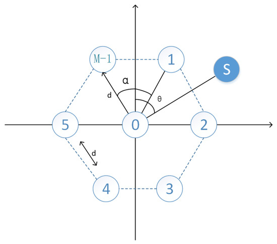
Figure 1.
Circular microphone array configuration.
The center microphone (i = 0) is defined as the reference point and the angle between the source and the vertical axis is θ. The time-delay of microphone i (i ≠ 0) relative to the center microphone can be denoted by
where d denotes the distance between the ith microphone and the reference point, α denotes the angle between two adjacent microphones, and c denotes the sound speed.
The phase transfer at each frequency is given by
where f denotes frequency.
The observed mixture signal in the frequency-domain is given by
where t denotes the time index, X(f,t) denotes the observed signal vector, S(f,t) denotes the source signal vector, and H(f) denotes the mixing matrix. They are given by
where T denotes the transpose, M denotes the number of microphones, and N denotes the number of sound sources.
Finally, the mixing matrix in Equation (6) is transformed into Equation (7) without considering echo and reverberation interference, as well as amplitude difference between two channels.
In a real speech environment, due to noise interference and reverberation, there may be some distortions in the mixing matrix.
2.2. Dimensionality Reduction
For a sufficiently populated array, the number of sound sources in the sound field can be assumed to be less than that of microphones, making voice mixing model a non-underdetermined problem. However, for separation algorithms like ICA, the number of separated signals is required to be equal to that of channels especially in the frequency domain, considering the permutation ambiguity. Therefore, dimensionality reduction is urged to be performed effectively. The most common method for dimensionality reduction is the PCA, which can be performed at each frequency bin.
Firstly, the cross-correlation matrix is calculated as
where L denotes the sample number and H denotes the conjugate transpose.
Second, the complex domain eigenvalue decomposition of the cross-correlation matrix is applied to obtain eigenvectors and eigenvalues corresponding to the components at the frequency bin. Then, the eigenvalues are ordered in descending order, d1 ≥ ⋯ ≥ dM, and M’ eigenvalues larger than the threshold [15] are selected to form a diagonal matrix D = diag(d1, ⋯, dM’). In addition, the corresponding eigenvectors are aligned to constitute the matrix E = [e1, ⋯, eM’]. The matrix for dimensionality reduction is given by
for which
where Z(f,t) is the dimensionality-reduced signal. Matrix V(f) whitens the observed signal, resulting in RZZ = I, and the dimension of signal Z(f,t) is M’, which is the number of the sound components contained at frequency f.
Normally, there are two important issues required to be considered through using of PCA. The first is the number of the reduced dimension. If the number of sound sources is previously known, the dimension of reduction could commonly be fixed to it. If not, some methods are necessary to calculate it. In this paper, we use two parameters, including threshold and number of sound sources, to determine the signal dimension at each bin. Second is normalization. In some studies, normalization of the observed signal at each frequency bin could be optionally applied before PCA dimensionality reduction, which will allow us to use a fixed threshold for dimensionality reduction at different frequency bins. However, the signal dimension after reduction at some frequency bins may exceed the number of sound sources, especially for the components with low SNR. If normalization is not applied, the process of dimensionality reduction with a fixed threshold could discard some noisy frequency components with low energy. Therefore, normalization before dimensionality reduction depends on the signal characteristics and processing strategies. In this paper, the signal is not normalized before applying PCA.
2.3. Speech Separation Using ICA
After dimensionality reduction by using PCA, any ICA algorithm for instantaneous mixtures can be employed at each frequency bin independently, such as the information maximization approach [16] combined with natural gradient [17], FastICA [18], or JADE [19]. In this paper, the information maximization approach combined with natural gradient is used.
Firstly, the ICA iteration is expressed as
where W is the iterative separation matrix, η is the step size, k is the iteration index, Y(f, t) = Wk(f) × Z(f,t) is the separation signal obtained by the kth iteration matrix, < >r denotes the time averaging, and ϕ(·) denotes a nonlinear function defined as
where Re(·) and Im(·) denote the real and imaginary parts of their arguments, respectively.
Then, the determinant of an expression of nonlinear correlation determines the end of the iteration, which is expressed as
where det(·) denotes the determinant.
When the nonlinear correlation of the signal is below the threshold or the iteration step exceeds the set threshold, the iteration of ICA stops. Furthermore, because of the independently iteration of ICA at each frequency bin, the scaling ambiguity and permutation ambiguity should be solved. As modeled in Section 2.1, the center microphone is defined as the reference point, so the timeline of the center microphone is used as a benchmark. Here, the W+(f) is defined as the Moore–Penrose pseudoinverse of W(f) × V(f). Then, the scaling ambiguity is therefore decided by
where Wr1+(f)denotes the first row of W+(f).
There are many methods to solve the permutation problem of FDICA [12], such as the directivity of separation matrix and the correlation of separation signal. Besides, independent vector analysis (IVA) could also solve this permutation problem, but it requires too much time to converge. In this paper, the permutation problem is solved by setting the initial value of W(f), which will be discussed in the next section.
3. Proposed Speech Separation Algorithm
Generally, speech separation algorithms based on a microphone array can be divided into two categories based on whether the sound source position, related transfer function (RTF), or steering vector is required. The representative methods of these two categories are beamforming and ICA in blind source separation (BSS). Beamforming is the most common speech enhancement algorithm based on microphone array measurements, which has the advantages of being easy to implement and a low computation cost, whereas the performance of beamforming depends on the accuracy of the sound source localization, especially in the scene where the interference sound source exists. To completely and accurately suppress the interference, the algorithms not only need the positioning information, but the steering vectors or even RTF which is hard to estimate [20]. From the perspective of actual implementation and use of BSS algorithms like ICA or complex Gaussian mixture model (cGMM), the sound source localization algorithms may not be essential. However, such algorithms are often cumbersome in actual applications. First, ICA obtains the separation matrix by iterating the objective function, which notably increases the computation cost. Although there are online stochastic gradient descent algorithms for ICA, the convergence rate is still a problem. Second, algorithmic modeling is not flexible to handle with the scenes of sound sources joining and moving. Third, without counting and localization algorithms, only using PCA for dimensionality reduction, it is difficult for BSS algorithms to iteratively converge in an appropriate dimension. Because of the sparsity of the speech signals in the time-frequency domain and the presence of noise, PCA could retrieves a dimension reduction that less than the existing number of sound sources and more than the existing number of sound sources, respectively. The different dimensions across the frequency bins lead to increased difficulty in subsequent process of permutation problem. Iterating in high dimension also leads to increased computation costs, especially for IVA, which iterates simultaneously at all frequency bins.
Therefore, an adaptive fast speech separation algorithm based on multiple sound source localization as preprocessing to select between beamforming and frequency domain ICA according to different mixing conditions per frequency bin is proposed in this section. Moreover, the proposed framework is not limited to ICA, IVA, cGMM, or other algorithms that iterate with a large computation cost can also use it to reduce calculation cost. Furthermore, the proposed method is not sensitive to the inaccuracy of the positioning result.
3.1. Counting and Localization of Multiple Sources
Multiple sources localization should be used to determine the number of sound sources, their angle, and the approximate mixing process in a speech environment [21,22,23]. In this section, the frequency-divided beamforming is used to locate multiple sound sources, which in fact is a simplified version of the method in [22], and the circular integrated cross spectrum (CICS) is replaced with delay-and-sum beamforming (DSB). This modified localization algorithm costs less computation while maintaining decent performance.
First, different signals occupy specific frequency bands is assumed due to the time frequency sparsity of speech signals [24]; therefore, each time and each sub-band frequency dominated by only one sound source is called the single-source analysis zone [25], for which it is easy to acquire the source angle by searching the direction with the maximum beam power. In this paper, the frequency band with multiple sound sources is not analyzed, but only single-source analysis zone to achieve multiple sound sources localization based on frequency division. To determine if a sound source on a frequency band is single, the energy cross-correlation between channels should be calculated as [21]
where i and j denote indices of microphones in an array; f is the frequency bin in frequency band Ω; Xi(f,t) is the signal acquired by microphone i in the frequency domain; Xj(f,t)* is the conjugate of the signal acquired by microphone j in the frequency domain; and |.| denotes the absolute value.
Then, the normalized energy cross-correlation between channels i and j is calculated by
Second, a threshold to the cross-correlation is applied to wipe off the frequency bands those do not belong to the single-source analysis zone, where beamforming can be applied to determine the angle of the sound source by obtaining the maximum power along the azimuth [26],
where P is the beam pattern; m is the microphone index; q is the angle of the beamformer; fΩ is the frequency bin with the highest energy in frequency band Ω; and τ is the time delay between the signal received by the m-th microphone and the array center in the direction of q. The scanning range of q is 360° on the horizontal direction of the microphone array and the scanning interval is 1°. Angle is estimated as
The angle of every single-source analysis zone is determined using the above-mentioned equations and then a global positioning result over all the frequency bins and time frames are obtained. By detecting the histogram of the positioning result, the number of sound sources and the azimuth of each source are both achieved. Figure 2 depicts the process of counting and localization of multiple sources.
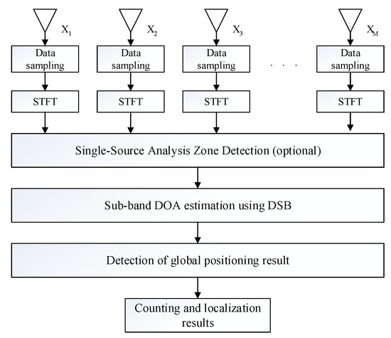
Figure 2.
Flow chart of counting and localization of sound sources.
3.2. Speech Separation According to Different Mixing Condition
Based on the results of PCA and positioning algorithm at each frequency bin, our algorithm starts to separate the mixed signal and there are three cases which are described in detail as followings.
3.2.1. Case I: M’ < N
The number of components at frequency bin is less than the number of existing sound sources because of the sparsity of speech signal in the time-frequency domain.
First, when M’ is equal to 1, the dimension reduction is not conducted. To minimize the computation cost and prove the effectiveness of the proposed framework, only the simplest DSB is used in this situation [27], where the attribution of signal components should be judged because the number of speech components is less than the number of existing sound sources. In Section 3.1, beamforming has been performed in each frequency bin, and the source angle in each frequency band is determined by searching the maximum beam power over the possible directions. Here, we use a similar method to determine the attribution of components by pointing the beam towards the estimated positions of sound sources. Then, the first M’ beams with the highest energy are the activated sound sources in current frequency bin. Then, the matrix of DSB is expressed as
where H1(f) is the column of Equation (7) corresponding to the source with the highest beam energy, Beam is the signal generated by the beamformer, and B is the beamformer coefficient.
The sound sources at other angles are set to zero at this frequency bin, then the processing matrix can be expressed as
where B(f) is arranged in the row corresponding to the source with the highest beam energy.
Second, if M’ > 1, the fixed beamforming is not effective enough for separation because of interferences, therefore ICA can be used. Then, the processing matrix can be expressed as
where WICA(f) can be calculated by Equations (11) and (14), which contains M’ rows, and what should be noted is that WICA(f)·V(f) is not continuously arranged in W[2] (f), similar to Equation (21), but each row corresponds to the M’ sound source with the highest beam energy.
3.2.2. Case II: M’ = N
It is the most common situation that the number of speech components is equal to the number of sound sources. ICA can be used normally, and the processing matrix is expressed as
where W[3] (f) contains N rows.
3.2.3. Case III: M’ > N
This case means the number of signal components is more than the number of sound sources; in this paper, the case where the localization algorithm fails to detect some sound sources is not considered, because the energy of these sound sources are much lower than other sound sources which have been counted and localized. These undetected sound sources are taken as ambient noise and still reduce the dimension to N. In this situation, the low-energy sound sources and the received noise of microphones will be compressed into the signal space by PCA, and then, ICA can be used. The processing matrix is the same with Equation (23).
Furthermore, due to the theoretical limitation of ICA, the permutation and scaling ambiguity should be solved after iteration in Case M’ > 1. This permutation ambiguity can be solved by postprocessing methods such as spatial directivity and correlation between frequency bins. However, these methods will increase computation load. In the set-up of Section 4.1, the postprocessing [12] costs ~0.2 s. Therefore, a proper initialization for iteration is found to control the convergence point so that the permutation will not be changed. In Section 4.1, the simulation results show that this approach is effective in the environment with reverberation time T60 = 0.3 s. For more adverse environments, the postprocessing is still recommended.
First, after the dimensionality reduction using PCA, the signal at each channel can be expressed as
where H(f) is an approximation of the real propagation process.
Then,
Therefore, by setting matrix P−1(f) as the initial matrix for ICA, the ICA iterative process can be performed. When H(f) is close to the real propagation process, the permutation is highly likely to remain unchanged.
Here, the scaling ambiguity can be solved by Equation (14). Considering the calculations of the Moore–Penrose pseudoinverse, a simple method is proposed to handle with the scaling ambiguity. By using the approximation of Equation (26) and the initial matrix, the separation matrix P−1(f) is replaced by WICA(f), and Y(f,t) is approximately equal to
where I’(f) maintains the permutation but the scaling of the components has been changed. We restore the scaling of the separated signal by
where/denotes element-wise division and diag(·) denotes the diagonal elements.
Because the result of the dimensionality reduction with PCA is directly related to the threshold of eigenvalue, the ratio among W[1] (f), W[2] (f) and W[3] (f) can be adjusted with the PCA threshold. According to the simulated result in Section 4.2, the processing method is modified when M’ > 1, and W[2] (f) is merged into W[3] (f). Therefore, by sorting the second largest eigenvalue of all frequency bins, the proportion of different processing schemes can be effectively controlled. Finally, the separated signals of each sound source over all frequency bins are integrated into a complete representation in the time-frequency domain, and converted into the time domain by applying the inverse Fourier transform. Figure 3 depicts the flow of speech separation according to mixing conditions.
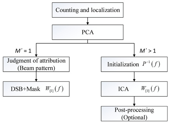
Figure 3.
Flow chart of speech separation according to mixing conditions.
4. Simulations and Experiment
4.1. Simulation Set-up
To evaluate the proposed speech separation algorithm, a series of simulations was conducted. Voice propagation in a multi-channel environment was simulated by calculating the impulse response between the sound source and each microphone and convolving the impulse response with the sound source signal to obtain the voice signal received by each microphone. The image-source model (ISM) [28,29] is used to calculate the impulse response of indoor speech propagation and signal convolution. For the multiple sound sources, each sound source was individually convoluted and generated, and then the signals were summed at each receiving microphone. The program was coded and ran in Matlab. The computer configuration is CPU: i7-5700, GPU: Nvidia 630, and 8GB memory. Configurations for the proposed method are shown in Table 1.

Table 1.
Configurations for proposed method.
Figure 4 depicts the considered indoor environment, which consists of Room A with dimensions 10 m × 10 m × 4 m, Room B with 6 m × 4 m × 3 m and reverberation time T60 = 0.3 s.
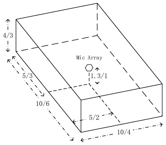
Figure 4.
Indoor environment for evaluation of speech separation.
The proposed method was evaluated for two, three, and four sound sources distributed according to Figure 5 and measured the improved signal-to-interference ratio (SIR) to estimate the algorithm performance.
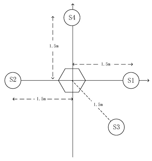
Figure 5.
Distribution of sound sources to evaluate the proposed speech separation algorithm.
The SIR of the sound source i at the receiving microphone j is given by
and the SIR after separation is given by
where yii is the component of sound source i and yik is the residual component from the other sound sources after separation. The SIR improvement defines the algorithm performance as
where the input SIR is calculated from the signal received by the microphone at the array center. Note that this performance measure only reflects the degree of separation considering the signal power, rather than the quality and completeness of the recovered signal.
4.2. Simulations
In Simulation I, two sources are randomly chosen from the given four sources in Figure 5 and speech separation is conducted with the proposed algorithm. Because the proposed method can switch between ICA and beamforming according to mixing conditions at each frequency bin, its influence on separation performance should be researched. Therefore, the SIR improvement was calculated with Equation (33) when the usage ratio of ICA increases from 0% to 100%, and the simulated result is shown in Figure 6 for Room A and Figure 7 for Room B, where the horizontal axis denotes the usage ratio of ICA in percentage; the vertical axis denotes the SIR improvement by using the proposed method. The selected source compositions are SET1 in which Source 1 located in 90°and Source 2 located in 270°, SET2 in which Source 1 located in 90°and Source 4 located in 0°, SET3 in which Source 1 located in 90° and Source 3 located in 150°, and SET4 in which Source 1 located in 90°and Source 3 whose theoretical position is decreased to 135°.
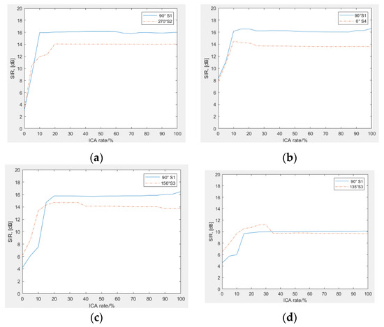
Figure 6.
Signal-to-interference ratio (SIR) improvement with separation under dual sources in Room A. (a–d) correspond to SET1-SET4, respectively.
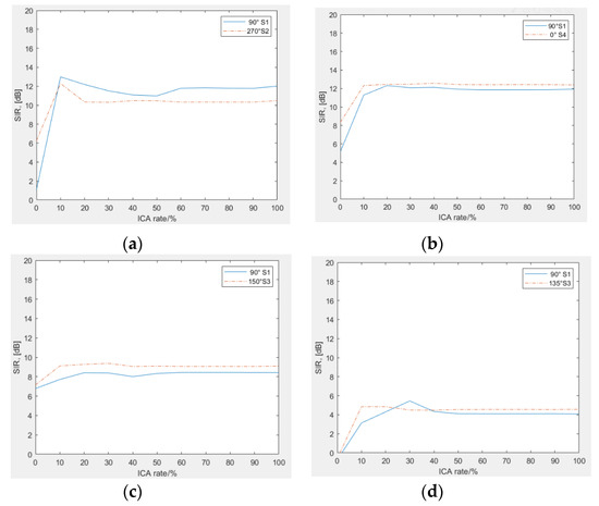
Figure 7.
SIR improvement with separation under dual sources in Room B. (a–d) correspond to SET1-SET4, respectively.
In Figure 6 for Room A, (a) is the separation result for SET1 when the localization result is 90° and 270°; (b) is the separation result for SET2 when the localization result is 89° and 0°; (c) is the separation result for SET3 when the localization result is 91° and 149°; and (d) is the separation result for SET4 when the localization result is 91° and 133°.
In Figure 7 for Room B, (a) is the separation result for SET1 when the localization result is 89° and 269°; (b) is the separation result for SET2 when the localization result is 89° and 0°; (c) is the separation result for SET3 when the localization result is 93° and 152°; and (d) is the separation result for SET4 when the localization result is 92° and 135°. Table 2 contains the simulated result of different cases.
Table 2.
Results by proposed method under dual sources in Room A and Room B.
From the simulation results, the following conclusions can be obtained.
- (1)
- The localization result of our preprocessing method is accurate, and the largest deviation from the actual position is 3° in Room B. The accuracy of the localization algorithm has a slight relationship with indoor environment due to the reverberation.
- (2)
- Increasing the usage ratio of ICA improves the performance of our proposed algorithm. When ICA is employed more than 30%, the algorithm performance tends to be flat, suggesting that nearly 70% of the frequency components in the mixed signal are dominated by a single sound source and the other components contain signal mixtures.
- (3)
- (4)
- The indoor environment has a strong impact on separation performance. In Room A, the highest SIR improvement is about 16.8 dB, whereas for the lowest case, it is 10.2 dB. In Room B, the highest SIR improvement is about 13.0 dB, whereas the lowest SIR improvement is 4.8 dB. The intensity of the reverberation increases as the size of room decreases, so that the performance of separation degrades.
- (5)
- The angle between two sources is 180°, 90°, 60°, and 45°. Therefore, the performance of our proposed algorithm decreases with angle interval because of the use of the initialization of ICA separation matrix. The performance of separation is more susceptible to the angle between sources in the smaller room. In our simulation, the angle interval could not be less than 45°, otherwise it can be considered that the effective separation function is lost.
In Simulation II, three sources were chosen from the given sources in Figure 5 and were used to conduct speech separation with the proposed algorithm. The selected sources composition is Source 1 located in 90°, Source 3 located in 150°, and Source 2 located in 270°. The localization result of the preprocessing step is 91°, 149°, and 270° in Room A and 92°, 153°, and 269° in Room B, respectively. The separation evaluation is shown in Figure 8, Figure 9 and Figure 10, where the horizontal axis is the usage ratio of ICA; the vertical axis is the SIR improvement by using the proposed method.
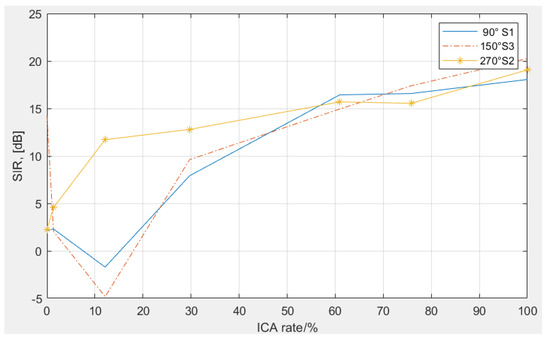
Figure 8.
SIR improvement with separation under three sources in Room A.
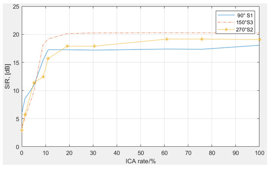
Figure 9.
SIR improvement with modified separation under three sources in Room A.
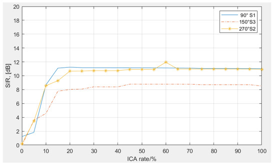
Figure 10.
SIR improvement with modified separation under three sources in Room B.
In this simulation, with increasing the usage ratio of ICA, the SIR improvement of the proposed algorithm is not always increasing as expected, it fluctuates at some positions. Furthermore, the increasing speed of SIR improvement is slower than that of the previous simulation. The reason is that for multiple components at a frequency bin, when the dimension of ICA iteration is determined by the PCA and it is less than the number of real sound sources, the iterative convergence of ICA could reach a bad point, causing the SIR improvement decreases. Therefore, a modification has been made to the frequency with multiple components, where the PCA is still used to reduce dimensionality; however, the ICA iteration dimension is equal to the number of real sound sources when the result number of PCA is less than the number of sound sources. Therefore, the threshold of PCA does not influence the effective convergence of ICA. The final separation result of the modified algorithm is shown in Figure 8 and Figure 9, where the problem in Figure 7 has been solved. The SIR improvement increases with increasing the usage ratio of ICA, and its maximal value is larger than 16 dB in Room A, 8 dB in Room B when ICA is employed 20%.
In Simulation III, all sources were chosen in Figure 5, and conducted speech separation with the proposed algorithm. The localization angles are 90°, 151°, 270°, and 1° in Room A, 91°, 155°, 269°, and 0° in Room B, respectively, and the SIR improvement is shown in Figure 11, Figure 12 and Figure 13, where the horizontal axis is the usage ICA ratio; the vertical axis is the SIR improvement by using the proposed method.
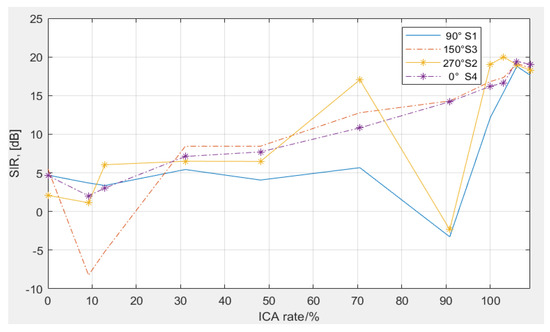
Figure 11.
SIR improvement with separation under four sources in Room A.
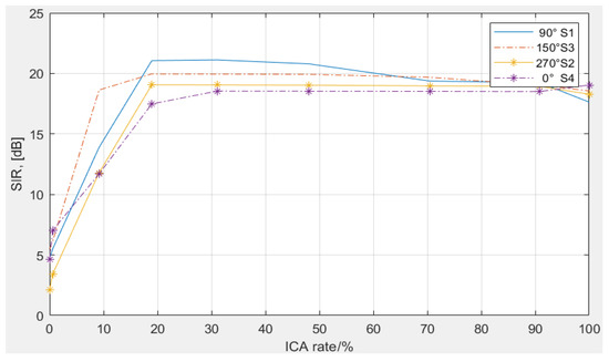
Figure 12.
SIR improvement with modified separation under four sources in Room A.
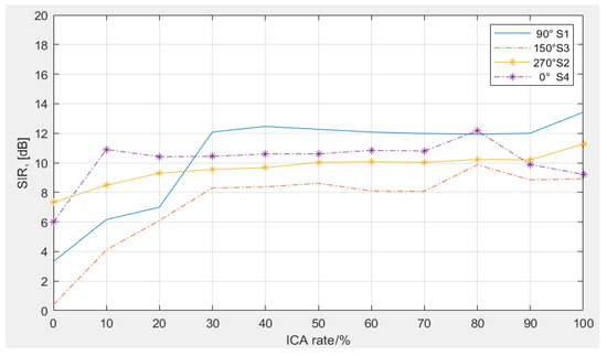
Figure 13.
SIR improvement with modified separation under four sources in Room B.
In Figure 13, the performance improvement of the proposed method is slightly slower than the previous situations, because in a strong reverberation environment, the sparsity of speech signals in the time-frequency domain is reduced.
Finally, the computation time with different number of sound sources was used to evaluate the processing ability with respect to multiple sources separation, and the time of separation is shown in Figure 14.
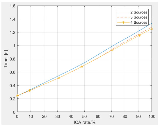
Figure 14.
Computation time of separation with different number of sound sources.
From Figure 14, the following conclusions are obtained.
- (1)
- For the separation with different number of sources, the computation time of our algorithm is approximately the same. The relationship between the computation time and the usage of ICA is approximately linear.
- (2)
- The computation time of our localization is ~0.49–0.63 s and is slightly proportional to the source number due to the process of detection of positioning result, whereas the computation time of our separation has little correlation with the source number.
- (3)
- Considering the signal length which is 1.1 s in our simulation, the computation time using the ICA increases by approximately 1 s compared with the DSB-based approach. With speech segments of other lengths, the ratio of the running time of the localization algorithm and the DSB to the length of the speech is almost constant. Moreover, when processing the longer speech, the ratio of the FDICA to the length of the speech could decrease slightly under the situation where the sound source and environment are basically unchanged. If the usage ratio of ICA is controlled to ~20%–30%, the total computation time of the localization and separation together is less than the length of the processed signal when an ideal separation result is obtained, which means the real-time processing is possible.
4.3. Experiments
In the experiment, the proposed method tested in a real indoor environment which is a classroom with size of 8 m × 6 m × 3 m, approximately. The speech is acquired by the xCORE Array Microphone, conducted by XMOS, which features 7 MEMS microphones with PDM output. There are two persons around the microphone array. Their positions are about S1 and S2 in Figure 5. The usage ratio of ICA in proposed method is 30%. Figure 15 is the spectrum of mixed signal received by the center microphone.
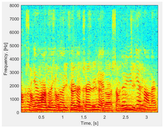
Figure 15.
Spectrum of the mixed speech received by center microphone.
The localization result is 97° and 273°. Figure 16 and Figure 17 are the spectrum of the separated speech, respectively. In Figure 16, there is an obvious sparse band near 2.8 kHz, due to the use of the DSB with a mask in the proposed method. The method determines that these frequency components belong to the second sound source, and does not use the FDICA algorithm for separation. The separated signals have only a small loss in the time domain expression. Compared with using 100% FDICA, the time of separation decreases from 3.31 s to 1.13 s. The time of localization is 1.46 s.
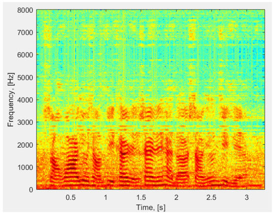
Figure 16.
Spectrum of the separated speech by a male.
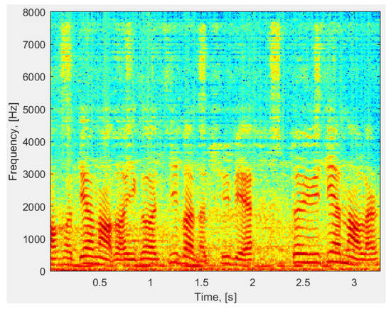
Figure 17.
Spectrum of the separated speech by a female.
5. Discussions
In the simulations and experiment, the proposed algorithm relied on ICA and DSB. The DSB algorithm can be replaced by the fixed beam coefficients with better spatial directivity or adaptive beamforming that can outperform the DSB-based approach in the low use ratio of ICA. The usage ratio of ICA to DSB in the algorithm is determined when sorting the second largest eigenvalue of all the frequency bins, rather than setting a threshold for the PCA.
As the number of the sound sources increases, the performance obtained from ICA and DSB slightly varies. In practice, the longer FFT length, such as 2048 points, is recommended when the number of sampling is sufficient for iteration of ICA. Because longer FFT length means higher frequency resolution, it is easier to satisfy the assumption of sparsity of speech signals in the time-frequency domain.
The switching mechanism in the proposed method is valid in different environments; however, the performance of separation is significantly degraded in smaller indoor environment because of the strong reverberation. Using the de-reverberation method, such as the generalized weighted prediction error (GWPE), as preprocessing is an effective approach to increase the upper limit of separation in a strong reverberation environment. However, the time spent is almost intolerable in real-time applications.
Through the total running time of proposed method in this paper could be less than the length of the processed signal by controlling the proportion of ICA, the separation result is late to the original signal about 1 s in real-time applications. The signal cannot be processed by frame because the ICA needs supple samples to iterative converge. When the speaker is not moving and the environment is basically unchanged, iterating ICA by using stochastic gradient descent is a commonly available method after converging of the proposed method. In real-time application, processing the blocks which contain several frames is a feasible approach which considers the real-time and tracking properties of the proposed method and initialization of several blocks in the beginning is still required.
6. Conclusions
We propose an adaptive and fast speech separation based on ICA and beamforming. The maximum number of mixed speech components per frequency bin is determined by using a positioning algorithm to prevent false sound sources. Then, the separation matrix of ICA is initialized according to sound source localization to notably reduce the iteration time and avoid ambiguity of permutation. PCA dimension reduction allows weighing the beamforming and ICA application for speech separation in real environments. Simulation and experimental results of multiple tests verify the high performance of the proposed algorithm.
The beamforming algorithm in the proposed method only uses the simple DSB-based approach when ICA is not necessary. In future work, we will explore methods to improve the algorithm performance when sound sources are located as similar angles, which is a common situation in real environments.
Author Contributions
K.Z. and Y.W. (Yangjie Wei) conceived and designed the study. K.Z. and D.W. performed the experiments. K.Z. and Y.W. (Yangjie Wei) wrote the paper. K.Z., Y.W. (Yangjie Wei), D.W. and Y.W. (Yi Wang) reviewed and edited the manuscript. All authors have read and agreed to the published version of the manuscript.
Funding
This research was funded by National Key R&D Program of China, grant number2018YFB1307500, the Natural Science Foundation of China under Grant, grant number 61973059 and 61532007.
Conflicts of Interest
The authors declare no conflict of interest.
References
- Hyvärinen, A.; Oja, E. Independent component analysis: Algorithms and applications. Neural Netw. 2000, 13, 411–430. [Google Scholar] [CrossRef]
- Amari, S.I. A new learning algorithm for blind separation of sources. Ad. Neural Inf. Process. 1996, 8, 757–763. [Google Scholar]
- Saruwatari, H.; Kurita, S.; Takeda, K.; Itakura, F.; Nishikawa, T.; Shikano, K. Blind Source Separation Combining Independent Component Analysis and Beamforming. EURASIP J. Adv. Signal Process. 2003, 2003, 1135–1146. [Google Scholar] [CrossRef]
- Cox, H.; Zeskind, R.; Owen, M. Robust adaptive beamforming. IEEE Trans. Acoust. Speech Signal Process. 1987, 35, 1365–1376. [Google Scholar] [CrossRef]
- Schmidt, R. Multiple emitter location and signal parameter estimation. IRE Trans. Antennas Propag. 1986, 34, 276–280. [Google Scholar] [CrossRef]
- Merino-Martínez, R.; Sijtsma, P.; Snellen, M.; Ahlefeldt, T.; Antoni, J.; Bahr, C.J.; Blacodon, D.; Ernst, D.; Finez, A.; Funke, S.; et al. A review of acoustic imaging methods using phased microphone arrays. CEAS Aeronaut. J. 2019, 10, 197–230. [Google Scholar] [CrossRef]
- Maganti, H.K.; Gatica-Perez, D.; McCowan, L. Speech Enhancement and Recognition in Meetings with an Audio–Visual Sensor Array. IEEE Trans. Audio Speech Lang. Process. 2007, 15, 2257–2269. [Google Scholar] [CrossRef]
- Niwa, K.; Nishino, T.; Takeda, K. Encoding large array signals into a 3D sound field representation for selective listening point audio based on blind source separation. In Proceedings of the 2008 IEEE International Conference on Acoustics, Speech and Signal Processing, Las Vegas, NV, USA, 31 March–4 April 2008; Institute of Electrical and Electronics Engineers (IEEE): Las Vegas, NV, USA; pp. 181–184. [Google Scholar]
- Araki, S.; Mukai, R.; Makino, S.; Nishikawa, T.; Saruwatari, H. The fundamental limitation of frequency domain blind source separation for convolutive mixtures of speech. IEEE Trans. Speech Audio Process. 2003, 11, 109–116. [Google Scholar] [CrossRef]
- Merino-Martínez, R.; Luesutthiviboon, S.; Zamponi, R.; Carpio, A.R.; Ragni, D.; Sijtsma, P.; Snellen, M.; Schram, C. Assessment of the accuracy of microphone array methods for aeroacoustic measurements. J. Sound Vib. 2020, 470, 115176. [Google Scholar] [CrossRef]
- Ikram, M.; Morgan, D. Permutation inconsistency in blind speech separation: Investigation and solutions. IEEE Trans. Speech Audio Process. 2004, 13, 1–13. [Google Scholar] [CrossRef]
- Sawada, H.; Mukai, R.; Araki, S.; Makino, S. A Robust and Precise Method for Solving the Permutation Problem of Frequency-Domain Blind Source Separation. IEEE Trans. Speech Audio Process. 2004, 12, 530–538. [Google Scholar] [CrossRef]
- Sarradj, E. A generic approach to synthesize optimal array microphone arrangements. In Proceedings of the 6th Berlin Beamforming Conference, Berlin, Germany, 29 February–1 March 2016. [Google Scholar]
- Luesutthiviboon, S.; Malgoezar, A.M.; Merino-Martinez, R.; Snellen, M.; Sijtsma, P.; Simons, D.G. Enhanced HR-CLEAN-SC for resolving multiple closely spaced sound sources. Int. J. Aeroacoustics 2019, 18, 392–413. [Google Scholar] [CrossRef]
- Merino-Martinez, R.; Herold, G.; Snellen, M.; Dougherty, R.P. Assessment and comparison of the performance of functional projection beamforming for aeroacoustic measurements. In Proceedings of the 8th BeBeC (Berlin Beamforming Conference), Berlin, Germany, 2–3 March 2020. [Google Scholar]
- Sawada, H.; Mukai, R.; Araki, S.; Makino, S. Convolutive blind source separation for more than two sources in the frequency domain. Acoust. Sci. Technol. 2004, 25, 296–298. [Google Scholar] [CrossRef][Green Version]
- Buchner, H.; Aichner, R.; Kellermann, W. A generalization of blind source separation algorithms for convolutive mixtures based on second-order statistics. IEEE Trans. Speech Audio Process. 2004, 13, 120–134. [Google Scholar] [CrossRef]
- Hyvarinen, A. Fast and robust fixed-point algorithms for independent component analysis. IEEE Trans. Neural Netw. 1999, 10, 626–634. [Google Scholar] [CrossRef] [PubMed]
- Cardoso, J.F.; Souloumiac, A. Blind beamforming for non-gaussian signals. IEE Proc. F Radar Signal Process. 1993, 140, 362–370. [Google Scholar]
- Sarradj, E. Three-Dimensional Acoustic Source Mapping with Different Beamforming Steering Vector Formulations. Adv. Acoust. Vib. 2012, 2012, 292695. [Google Scholar] [CrossRef]
- Pavlidi, D.; Griffin, A.; Puigt, M.; Mouchtaris, A. Source counting in real-time sound source localization using a circular microphone array. In Proceedings of the 2012 IEEE 7th Sensor Array and Multichannel Signal Processing Workshop (SAM), Hoboken, NJ, USA, 17–20 June 2012; pp. 521–524. [Google Scholar]
- Pavlidi, D.; Griffin, A.; Puigt, M.; Mouchtaris, A. Real-Time Multiple Sound Source Localization and Counting Using a Circular Microphone Array. IEEE Trans. Audio Speech Lang. Process. 2013, 21, 2193–2206. [Google Scholar] [CrossRef]
- Griffin, A.; Pavlidi, D.; Puigt, M.; Mouchtaris, A. Real-time multiple speaker DOA estimation in a circular microphone array based on Matching Pursuit. In Proceedings of the 20th European Signal Processing Conference (EUSIPCO), Bucharest, Romania, 27–31 August 2012; pp. 2303–2307. [Google Scholar]
- Yilmaz, O.; Rickard, S. Blind Separation of Speech Mixtures via Time-Frequency Masking. IEEE Trans. Signal Process. 2004, 52, 1830–1847. [Google Scholar] [CrossRef]
- Puigt, M.; Deville, Y. A New Time-Frequency Correlation-Based Source Separation Method for Attenuated and Time Shifted Mixtures. In Proceedings of the 8 th International Workshop on Electronics, Control, Modelling, Measurement and Signals, Liberec, Czech Republic, 21–23 May 2017; pp. 34–39. [Google Scholar]
- Lim, H.; Yoo, I.-C.; Cho, Y.; Yook, D. Speaker localization in noisy environments using steered response voice power. IEEE Trans. Consum. Electron. 2015, 61, 112–118. [Google Scholar] [CrossRef]
- Alexandridis, A.; Griffin, A.; Mouchtaris, A. Capturing and Reproducing Spatial Audio Based on a Circular Microphone Array. J. Electr. Comput. Eng. 2013, 2013, 718574. [Google Scholar] [CrossRef]
- Lehmann, E.A.; Johansson, A.M. Diffuse Reverberation Model for Efficient Image-Source Simulation of Room Impulse Responses. IEEE Trans. Audio Speech Lang. Process. 2009, 18, 1429–1439. [Google Scholar] [CrossRef]
- Available online: http://www.eric-lehmann.com/ (accessed on 12 October 2018).


© 2020 by the authors. Licensee MDPI, Basel, Switzerland. This article is an open access article distributed under the terms and conditions of the Creative Commons Attribution (CC BY) license (http://creativecommons.org/licenses/by/4.0/).