Abstract
High-permeability distributed wind power and photovoltaic systems are connected to the distribution network, which exacerbates the volatility and uncertainty of the distribution network. Furthermore, with the increasing demand of heating in winter and environmental protection, the wide use of electric thermal storage heating equipment (ETSHE) can promote distributed renewable energy utilization. However, an unplanned ETSHE connection to the distribution network may cause serious power quality problems. A new method of equipment location and capacity is proposed, which considered the improvement of power quality and load demand characteristics of the distribution network. First, based on heat load portrait technology, the node’s thermal load classification prediction was carried out to provide the data basis for the model solution. Second, the multi-objective optimal location and capacity programming model including harmonic distortion rate, voltage deviation, voltage fluctuation, and ETSHE cost was established. Then, the system nodes were preprocessed based on the sensitivity analysis method to reduce the number of installation nodes to be selected, and a feasible alternative set of installation nodes for the optimal configuration model of ETSHE could be obtained. Finally, the improved multi-objective particle swarm optimization algorithm was used to solve the model, and the data envelope analysis method was used to evaluate the power quality of each access scheme. The analysis of the numerical example shows that it can not only satisfy the user′s heat demand, but also effectively improve the power quality by rationally planning the location and capacity of ETSHE, which achieves the safe and efficient utilization of energy.
1. Introduction
In recent years, large-scale use of fossil fuels has led to exacerbating the environmental pollution problems, thus energy reform is imperative. New energy power generation is widely developed worldwide, among them, distributed photovoltaic and wind power generation are widely used because they have the characteristics of abundant available resources and reliable devices [1]. However, from another perspective, distributed photovoltaic and wind power also have the characteristics of fluctuation and stochastic. When the output of a distributed photovoltaic or wind power connected to a node in the power distribution system exceeds the node′s self-consumption, the node voltage will exceed the limit. At the same time, a large number of distributed photovoltaics use power electronic equipment, which will bring a lot of harmonics to the distribution network, and can cause serious power quality problems [2,3]. Due to the intensification of environmental problems and the oversupply of electrical energy, electric thermal storage heating equipment, which holds the function of time shifting and storage of electrical energy, has been widely applied. In fact, the location and capacity of ETSHE is closely related to the characteristics of heat load. The characteristics of heat load mainly include the duration of heat load and the distribution of heat load within the day. There are various factors that affect load such as population, weather, and holidays, etc. The relationship between these factors and load is non-linear, which is even more difficult to describe and predict. The difference of energy use characteristics of thermal load brings new challenges to distribution network planning. For different thermal loads, the optimal configuration planning of ETSHE will also change accordingly, therefore, load portrait is the premise and foundation of optimal operation [4].
In light of the improvement of power quality, scholars at home and abroad have found that the goal of improving power quality can be achieved through the reasonable allocation of energy storage devices at corresponding nodes. However, traditional storage battery energy storage equipment, with poor peak-regulating capacity and high cost, cannot meet the needs of heat users. However, the storage of energy through the ETSHE can make good use of its time-shifting and storage characteristics to meet the multi-energy needs of users. However, the different access locations and capacity of the energy storage systems have a great influence on the power quality governance, so the choice of access location and the determination of capacity are problems that need to be solved urgently [5]. In [6], a constant capacity optimization model for energy storage equipment location was presented and solved by genetic algorithm. Meanwhile, the total cost was saved by adding the capacity correction link. In [7], a two-layer optimization method for multi-point distributed energy storage system location and fixed capacity in high photovoltaic penetration distribution networks was proposed. The authors in [6,7] only considered traditional electric energy storage. In addition to the basic energy storage planning presented above, some have also studied the energy storage planning method considering the demand characteristics. Such as [8], the proposed polygeneration microgrids system includes trigeneration plants, renewables, district heating, thermal and electrical storage systems and flexible loads, building demand-response model and storage systems model. Thermal storage proved to potentially have a very relevant impact on the microgrid operation, and the analysis also showed the potential reduction of the operating costs that could be achieved by demand-response. Furthermore, the authors in [9,10] realized the development of an energy management system (EMS), which was implemented and run at the smart polygeneration microgrid (SPM), that modified the existing EMS model and predictive control to take into account the existence of a thermal storage system with a suitable capacity. It is worth noting that the heat storage has been represented by resorting to a new battery-type model that is able to predict the transient behavior of the grid, according to the historical series of heat and electricity demand data during 2017. In such a way, it has been possible to calculate the optimal size of the thermal storage that maximizes the global saving. The study in [11] investigated the influence of energy storage location and capacity on the overall economy of the grid and wind energy utilization, where the premise is a third party owns the energy storage. However, this did not consider the improvement of energy quality caused by energy storage. In [12,13], according to the data collected by the power quality detection device, an appropriate evaluation method to calculate the power quality level of the access point after the energy storage system was connected. However, it did not combine the planning of the energy storage system with a power quality assessment.
In summary, considering the power quality and the impact of load characteristics, there are still few works concerning solving the location and capacity selection problem for ETSHE (not basic electric energy storage). Based on the above discussions, this paper proposed a method for selecting the location and capacity of the ETSHE connected to the distribution network, which avoids the disadvantages of high costs and the existence of pollution. The adaptive inertial weight improved particle swarm optimization (IMOPSO) method was proposed, which is suitable for distribution network systems with larger nodes. The influence of load characteristics on the planning was considered, thus the research results were closer to the actual situation. The model uses the power quality as the optimization target, which effectively solves the power quality problem caused by the new energy generation with high permeability.
The main contributions are introduced from four aspects, as follows:
- First, the minimum intra-class distance is used as the objective function to perform fuzzy clustering on the heat load. Second, on the basis of conventional forecasts, the influence weight of the meteorological factors on the outdoor temperature of the day is calculated to correct the outdoor temperature, improve the linear fitting goodness with heating heat load, and provide initial classified heat load data for the optimal configuration of ETSHE.
- The sensitivity coefficient is calculated based on the sensitivity radar chart and sensitivity calculation formula. The sensitivity discrimination of each node in the distribution network can effectively eliminate the nodes that do not meet the sensitivity and prevents the solution from falling into the wrong node, which can improve the efficiency and accuracy of the solution.
- Establish a location and capacity planning model for ETSHE and multi-objective functions including harmonic distortion, voltage deviation, voltage fluctuation, and energy storage equipment costs.
- In the planning stage, data envelopment analysis (DEA) is used to evaluate the power quality of access schemes with multiple indicators and single indicators, and an effective and unified method for distribution network planning and power quality assessment is proposed.
2. Load Characteristic Portrait
Traditional load forecasting methods generally only consider the typical daily curve of heat load, but not consider the differences in the heating characteristics of classified heat loads. Under the background of the rapid development of big data technology, portrait technology has been widely used in the fields of e-commerce and the internet [14]. This paper applied portrait technology to the extraction of heating user characteristics for the first time. In this paper, the thermal user load portrait was defined as follows. Different thermal loads were predicted by a high-precision prediction method so that the thermal loads were treated differently according to the different heating characteristics. To comprehensively consider the user heating characteristics and influencing factors, we established a user heating behavior label library. Based on the fuzzy C-means (FCM) algorithm for label clustering, different types of heating users used warming mode portraits, which makes the results of user heating behavior analysis more intuitive [15].
2.1. Clustering with Warm Behavior Patterns
The goal of users label clustering is to quickly grasp the heating characteristics of different thermal users to achieve different treatments of different heating groups. After combing and screening many times, the following six labels were obtained, as shown in Table 1.

Table 1.
Users label description.
In this paper, FCM clustering algorithm was used to calculate each thermal user’s label data to be clustered, and four memberships of thermal user clustering centers to realize the clustering division of the sample thermal user’s label data. During the iterative process, FCM takes the minimum intra-cluster distance and the maximum distance between clusters as the optimization goals, and constantly adjusts the categories of various thermal user data, so that it optimizes the clustering results continuously. The object to be clustered is the -dimensional dataset of samples:
The data collection class is divided into subsets, where the value of is 4, the subset is represented as ; and , and represent residents, education, business and industry, respectively. Here, we set = 7, which represents six items of user label data and one category data, respectively. Assuming that the probability of each thermal user belonging to the th clustering subset is , then FCM can be defined as an optimization problem with equality constraints [15]:
where is the value function of FCM. is the membership factor, which is used to adjust the degree of influence of the membership indicator in the optimization target. In most cases, we chose = 2. The iterative formulas for obtaining membership coefficients and cluster centers are shown in Equations (2) and (3) [15]:
Clustering steps of the warm behavior patterns for thermal users based on the FCM algorithm:
- Initialization: Set the number of clustering and membership factor m, randomly initialize the membership matrix , is a matrix made up of , the center of the cluster.
- Parameter update: According to Equation (2), calculate the clustering center of each label of thermal users; according to Equation (3), calculate the membership matrix of all thermal user labels and each clustering center , classify thermal users into the clustering center with the highest membership.
- Convergence judgment: If the change of the objective function is less than the preset threshold, then output the clustering result, otherwise return to Step 2.
- End of clustering: Save and display the clustering results.
2.2. Load Portrait
Load portrait refers to the method of high-precision prediction of the heating heat load by considering the main factors affecting heating load such as outdoor temperature, solar radiation, natural wind, etc. Correct outdoor temperature can be performed by using solar radiation and wind speed to improve the fit between outdoor temperature and thermal load [16]. Wind speed and solar radiation are the main factors affecting the heating heat load. The correction of wind speed for outdoor temperature can be converted into an equivalent cooling temperature [17]. The equivalent cooling temperature formula considering the influence of wind speed is shown in Equation (4):
where is the external wind speed value, ; is the equivalent temperature of wind speed cooling; °C. , and are the wind speed correction coefficients, where the values are 0.0246, 0.4525, 3.2398, and 7.23, respectively.
The correction of outdoor temperature by solar radiation can be converted into an equivalent heating temperature as shown in Equation (5):
where is the external light value; , is the light conversion coefficient; ; according to [17], we set the unit of as 100 .
is the uncorrected outdoor temperature. When considering both the outdoor wind speed and solar radiation of the day, the calculation formula for outdoor temperature is given as follows:
In order to improve the accuracy of forecasting heating load, this study not only considered the influence of wind speed and solar radiation on outdoor temperature of the day, but also considered the influence of wind speed and solar radiation on outdoor temperature of the past day. In this paper, we calculated the influence weight of previous meteorological factors on the outdoor temperature of the day to modify the outdoor temperature and linearly fit it with the heating heat load, so that their fitting goodness was further improved [18,19,20].
According to heat transfer knowledge, the influence of meteorological factors on the outdoor temperature of the day decreases with the increase in days. In order to facilitate the prediction of heating heat load, the influence of meteorological factors of all past days on the outdoor temperature of that day cannot be considered. Statistical results showed that heating heat load was related to meteorological factors of the previous 4–5 days. We used MATLAB programming to find the optimal days and the reasonable weight of past weather factors to correct the outdoor temperature of the day. When the outdoor temperature and the heating heat load were linearly fitted, the goodness of fit value was the maximum. This means that when the number of days considered is n days, the outdoor temperature of the day is given as follows:
where , , , represent the weight value of day , day − 1, day − 2, and day − n, respectively, and > > > …… > , and the sum of weight values is 1. is the outdoor temperature after solar radiation and wind speed correction of day − n, and is the outdoor temperature of day after correction on the current day and the previous day.
The “trial” method was adopted to determine the index weight of the influence of past meteorological factors on the outdoor temperature of the day to correct the outdoor temperature and obtain the relationship between the heat load and the temperature of the day, then obtained the relationship between the heat load and time. For example, if n = 2 in Equation (7), we can set , , and to simplify the calculation, and is an integer between 1 and 10.
3. Optimal Configuration Model of Electric Thermal Storage Heating Equipment
High-permeability distributed photovoltaic and wind power connected to the distribution network cause a series of power quality problems, which can be improved by installing ETSHE at appropriate nodes of the distribution network. However, the power quality of the power grid involves many aspects such as voltage and current. The location and capacity of the energy storage system needs to consider the effect of improving the power quality, the consumption of new energy, and the economics of the energy storage system. It is a multi-objective optimization plan model.
3.1. Objective Function
3.1.1. Total Current Harmonic Distortion
The fundamental current flowing through the power load is equal to the sum of the fundamental current of the power grid and the fundamental current of the inverter. When the power load is unchanged, the current harmonics are unchanged, but the fundamental current of the distribution network is reduced, and the total current harmonic distortion rate at the access point is increased. With the increase of access capacity, the total current harmonic distortion rate of the distribution network may exceed the range of grid access energy. Therefore, the total distortion rate of current harmonics was selected as one of the objective functions of the energy storage system location and capacity. The mathematical expression is [21]:
where is the root mean square value of the fundamental current and is the root mean square value of the -th harmonic current. Here, we set = 7, where only the 7th and lower harmonics were considered.
3.1.2. Voltage Deviation
Voltage is one of the most important indicators of power quality, and voltage deviation is a main indicator to measure the normal operation of the power supply system [22]. Distributed photovoltaic access to the distribution network can increase the voltage of the nodes, and excessive photovoltaic output will cause some nodes to exceed the limit. In this paper, the node voltage deviation was selected as one of the objective functions of the energy storage system location and capacity determination, its mathematical expression is [13]:
where is the voltage of node at time ; is the system standard voltage; and is the number of system nodes. is the number of detection moments.
3.1.3. Voltage Fluctuation
As the output power of the device is fluctuating, the voltage fluctuation caused by the connection to the distribution network is , so the voltage fluctuation was selected as one of the objective functions of this article. The mathematical expression is [23]:
where is the rated voltage; is the current change caused by the output power change at the access point; and is the equivalent impedance of the two-port network distribution network viewed at the access point.
3.1.4. Total Cost of Energy Storage System
The ETSHE must also consider the cost issue while ensuring the quality of the power. The total cost of the energy storage system was selected as one of the objective functions.
Equipment Cost of Electric Boiler
The equipment cost of an electric boiler is proportional to its rated heating capacity, which is equal to the design daily heat supply rating, thus Equation (11) is:
where is the unit price corresponding to the unit heat supply of the electric boiler. is the rated heat supply of the electric boiler. is a vector composed of the hourly heating capacity of the designed electric power boiler.
Equipment Cost of Heat Storage Body
The cost of the heat storage equipment is proportional to the volume of the equipment, then , and are the unit price and volume of the heat storage body, respectively.
Equipment Cost of Heat Storage Pump
The key parameters of heat pump selection are head and flow. The head is only related to the building structure and was selected according to typical values, and the heat pump investment was proportional to the rated flow at a certain head [24,25]. Therefore, the heat pump equipment cost can be expressed by Equation (12):
where is the increased equipment investment for each additional unit of the rated flow of the heat pump. is the safety factor when calculating the rated flow, in this paper, is the conversion constant of kilowatt hours and joules, here . is a vector formed by designing the hourly direct supply ratio of the electric power boiler, and are the specific heat and density of the heat medium. The difference in heat storage temperature is usually [26].
Equipment Cost of Control Device
The equipment cost of the control device is related to the complexity of the electric boiler system. It was found that the equipment cost of the control device is basically proportional to the rated heating capacity of the heating device of the electric boiler, which is shown as follows:
where is the investment cost of the control device for each additional 1 kW of the rated heating capacity of the electric boiler.
This article does not consider the operation and maintenance costs of energy storage equipment, only the investment and installation costs of energy storage equipment were considered, so the total cost of ETSHE is given as Equation (14):
where is the equipment installation cost coefficient. Usually, the equipment installation cost is about 20% of the total equipment cost, so we set = 1.2.
Therefore, the location and capacity multi-objective optimization model of the energy storage system comprehensively considered the voltage deviation of the distribution network nodes, the total distortion rate of the current harmonics, the voltage fluctuation, and the total cost of the energy storage system. The objective function is shown as Equation (15):
where is the normalized weight coefficient.
3.2. Restrictions
3.2.1. Equality Restrictions
1. Power flow constraint equation
The initial power flow calculation of the planned distribution network is performed, the voltage value and active power of each node are calculated. The power flow constraint is as follows [27]:
where and are the active and reactive power injections at node . and are the voltage amplitudes of nodes and . and are the conductance and susceptance of branch . is the voltage phase angle difference between the -th and -th node.
2. The hourly balance of heat supply and heat demand is:
where is a vector formed by the design of the hourly direct supply ratio of the electric power boiler. is the vector for designing the hourly heating capacity of the electric power boiler. is the heat provided by the heat storage body to the user during period . is the maximum design daily heat load. is the ratio of the heat load to the maximum value for the days on the design day.
3. The thermal equilibrium equation of the heat storage body is:
where is the amount of heat stored in the heat storage body at the beginning of time t.
3.2.2. Inequality Constraint
1. The maximum heat storage capacity is limited by the volume of the heat storage body:
where is the volume of the heat storage body, and and are the specific heat and density of the heat medium, respectively. is the conversion constant of kilowatt-hours and joules, here . Usually, the difference in heat storage temperature is °C. is the effective volume ratio of the heat storage body, which refers to the ratio of the volume that can actually contain the heat medium to the total external volume.
2. The upper limit of the heat supply of the heat storage body is:
3. The range of the value of the direct heat supply ratio of electric boilers is constrained as:
4. Constraints of voltage levels before and after the ETSHE is connected to the distribution network:
where and are the voltage level indicators before and after the energy storage is connected to the distribution network, respectively; is between 0 and 1.
5. Constraints on active loss before and after the ETSHE is connected to the distribution network:
where and are the active power loss before and after the ETSHE is connected to the distribution network, respectively. Similarly, is between 0 and 1.
The objective functions and constraints of the optimization model in this paper were grouped as shown in Figure 1:

Figure 1.
Optimization configuration model.
4. Node Sensitivity Analysis and Calculation Method
For power networks with a small number of nodes, the optimal configuration scheme for the location and capacity of ETSHE can be easily calculated by exhaustive methods. When the power network is complicated, there are many installation nodes available for installing energy storage at this time. If the optimal node is still selected according to the exhaustive method, the calculation of the optimal allocation scheme is large, which cannot be solved or the result falls into a local optimum. For this reason, the sensitivity analysis method was proposed to calculate the sensitivity coefficient of electric regenerative heating equipment installed at the node, and the node with higher sensitivity was selected as the alternative set of the installation node of ETHSE, which will greatly improve the optimal allocation efficiency of electrical thermal storage.
Sensitivity coefficient refers to the degree of sensitivity of the system, represented by state variables to changes in the control variables and disturbance variables [28]. For the electric storage thermal heating equipment location and capacity optimization configuration model, it refers to the sensitivity of the objective function of the optimal configuration to changes in energy storage installation capacity. The optimization objective of this paper is multi-objective function and the fundamental purpose of installing energy storage is to effectively control the power quality problem of the distribution system. When a large number of single-phase photovoltaic power sources are connected to the system, it will cause voltage three-phase imbalance problems. However, as single-phase photovoltaic power generation has not been widely used, it has little influence on the three-phase unbalance degree of power grid voltage. Therefore, only the three-phase imbalance is considered when defining sensitivity.
In a three-phase three-wire system, there is no zero-sequence component. For a three-phase system without a zero-sequence component, the simplified calculation method of the three-phase imbalance recommended by the national standard is as follows [29]:
where represents the three-phase negative sequence imbalance, and , , and represent the effective value of three-phase voltage, respectively.
In this paper, the radar chart analysis method was used to visually and comprehensively analyze and evaluate the sensitivity of the nodes. Finally, the nodes with higher sensitivity were selected as candidate nodes. The schematic diagram of the sensitivity radar is shown in Figure 2. The solid arrows in the figure indicate the power quality indicators; the value increases according to the arrow direction. The outer circle indicates the advanced level value of each indicator, which can be expressed by 1.5 times of the indicator standard value. The middle circle indicates the standard value of each indicator. The inner circle indicates the unqualified value. The dashed line indicates the actual value of each indicator. If the actual value is less than the standard value, this type of indicator is indicated by “−”. If the actual value is greater than the standard value, this type of indicator is indicated by “+”.
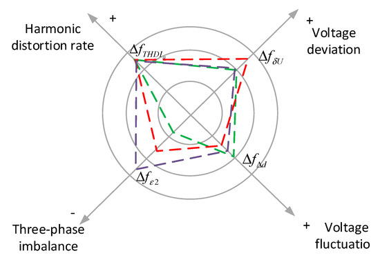
Figure 2.
Schematic of the sensitivity radar.
Therefore, in this paper, when the four power quality indicators of any node were defined as “−”, it was considered that the sensitivity of this node to power quality reached the standard and could be used as an alternative node. The specific calculation method is:
When the sensitivity coefficient = 1, the node can be used as a candidate node. If = 0, the node is eliminated.
The sensitivity coefficient reflects the degree of sensitivity of any node to the four aspects of harmonic content, voltage deviation, voltage fluctuation, and three-phase imbalance. If the energy storage system is installed at this node, the higher the value, the better the power quality will be. Therefore, by calculating the sensitivity coefficients of all nodes in the system, it is possible to find in advance a set of alternative nodes that are better at improving the power quality of the system, which can effectively reduce the number of computing nodes, greatly reduce the amount of calculations, and improve the optimization of the economy and efficiency of configuration.
Nodes are ranked according to the sensitivity coefficient, and higher-sensitivity nodes are preferentially selected to form an initial optimized candidate set. Subsequently, the heuristic optimization algorithm can be applied to solve the model quickly. This paper used the adaptive inertial weight IMOPSO algorithm to solve the model.
The main steps of the adaptive inertia weight IMOPSO algorithm are as follows:
- The network topology, switch state, node voltage range, distributed photovoltaic, wind parameters, and parameters of ETSHE in the distribution network system are initialized. The sensitivity coefficients of each node are calculated and sorted separately. The top 40% of the sorted nodes are selected to form a candidate set of installation nodes.
- The parameters such as the size of the particle swarm, the maximum number of iterations of the algorithm, the acceleration factor, the value range of the adaptive inertia weight, and the speed range of the particles are set in the improved particle swarm optimization.
- The particles in the candidate set are evaluated, and the fitness function value of each particle is calculated. After ranking, the individual optimal value and the global optimal value of the particles are determined and updated.
- Update the particle′s velocity and displacement, calculate the value of the adaptive inertia parameter.
- Check if the maximum number of iterations is exceeded. If it is exceeded, stop iteration and output the calculation result, otherwise skip to Step 3 to continue the iterative calculation.
In this algorithm program, the total current harmonic distortion rate, the sum of voltage deviations, the voltage fluctuations, the investment, and installation cost of the energy storage system are optimized objective functions. The number of iterations is the cycle control variable, and the location and capacity of the ETSHE are taken as decision variables. By improving the solution of the particle swarm algorithm, the optimal position and optimal capacity for the energy storage installation can be obtained.
The solution flow chart of IMOPSO algorithm in this paper is shown in Figure 3.

Figure 3.
Improved particle swarm optimization algorithm flowchart.
5. Simulation Analysis
This paper used IEEE-33 and IEEE-118 power distribution systems for verification, respectively, which were used to analyze the impact of high-permeability wind power and photovoltaic access on the power quality of the power distribution network. Through the rational optimization of flexible resources such as ETSHE, the power quality of high-permeability wind power and photovoltaic power distribution networks is improved.
5.1. Load Portrait Result
Using FCM clustering algorithm for label clustering, where the value of was 200 in this paper, we obtained four typical thermal users, as shown in Table 2. Figure 4 shows the distribution diagram of the FCM clustering results. According to the membership matrix in Figure 4, there were some differences in the characteristics of the four types of heating customers, but there were also some overlaps, which will affect the planning of the ETSHE. Equations (27) and (28) were used to calculate the fitting relationship between and , and the four types of typical users’ heat consumption over time were further calculated, as shown in Figure 5. The results of the thermal load portrait were input into the PSO as the initial data.
Table 2.
Four types of customer label characteristics.
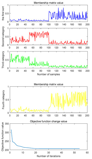
Figure 4.
Fuzzy c-means clustering results of four types of users.

Figure 5.
Energy consumption characteristics of the four typical users.
It can be seen from the results that when considering the influence of meteorological factors on the outdoor temperature of the day in the past two days, the goodness-of-fit of the linear fitting with the heating heat load was a maximum value after the correction of the meteorological factors on that day. It shows that the curve at this time can best reflect the relationship between and , and the value of can be predicted from the modified . For this set, the heating heat load can be predicted by the following formula:
The predicted values of different heating heat loads were obtained from Equations (27) and (28). Within a day, the temperature changes with time, and the heating heat load changes with air temperature, so the curve of the heating load with time can be obtained equivalently. The energy consumption characteristics of four typical users are shown in Figure 5, where the typical users′ energy consumption characteristic curves show different trends.
5.2. Simulation Scenario Setting
We used two scenarios to analyze the effects of the optimal scheduling of electrical thermal storage heating equipment and load demand characteristics on the improvement in the power quality of the distribution network.
Scenario 1: In the absence of flexible resources, the indicators of power quality include high-permeability wind power and photovoltaic power distribution networks.
Scenario 2: In the case of ETSHE and load demand characteristics affecting the optimal dispatching scenario, various indicators of power quality include high-permeability wind power and photovoltaic distribution networks.
5.3. IEEE-33 System Simulation Analysis
1. Basic data
The distribution network load, photovoltaic, and wind power data are shown in Table 3. The installation locations of wind power and photovoltaic are shown in Figure 6. The distribution network contains twelve distributed photovoltaics with a capacity of 0.5 MW, which are connected to nodes 2, 4, 6, 8, 10, 12, 14, 16, 18, 20, 22, and 24. At the same time, the distribution network also contained four distributed wind power generation with a capacity of 0.5 MW, which were connected to nodes 26, 28, 30, and 32. In order to ensure the maximum consumption of renewable energy, each distributed power supply is operated with actual output.
Table 3.
Load, wind power and photovoltaic power of a typical day (MW).
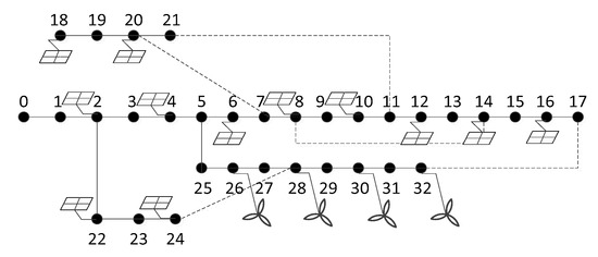
Figure 6.
IEEE 33-node power distribution system wiring diagram.
2. Result analysis
(1) Optimal scheduling results of ETSHE considering load characteristics
In principle, the nodes that can be connected to ETSHE are 1–32, but harmonics, voltage deviations, and voltage fluctuations caused by high-permeability distributed wind power and photovoltaic will cause some nodes to cancel each other out. Considering the objective function, the node sensitivity analysis method was applied, and the set of nodes for energy storage access included five nodes: nodes 4, 8, 13, 25, and 31. In order to highlight the impact of load characteristics on optimal planning settings, we considered that nodes 4 and 13 were residential loads, node 8 was a commercial load, node 25 was an industrial load, and node 31 was an educational load.
According to the optimization model constructed in this paper, the IMOPSO algorithm was used to solve the calculation example. The population size of the IMOPSO algorithm was 80, and = 0.5, = 0.8, [30,31]. The installation position and capacity of the electric regenerative heating equipment are shown in Table 4.
Table 4.
Optimized Configuration Results.
(2) Node sensitivity analysis before and after comparison
As can be seen from Table 5, the range of optimized nodes is effectively reduced and the effectiveness of the solution is greatly improved by the use of the node sensitivity analysis method.
Table 5.
Comparison analysis before and after node sensitivity analysis.
(3) Power quality improvement analysis
Through the optimization of two flexible resources, the power quality of distributed wind power with high penetration and photovoltaic power distribution networks has been significantly improved. Figure 7, Figure 8 and Figure 9 are the comparison curves of the total current harmonic distortion rate, voltage deviation, voltage fluctuation of the distribution network with high penetration wind power, and photovoltaic access in two scenarios. Line charts show the comparison of different scenarios of node power quality indicators, and the bar charts show the percentage improvement of the two scenarios relative to the national standard value.
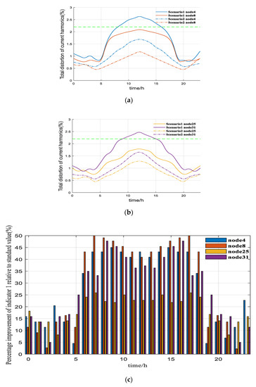
Figure 7.
Current harmonic distortion rate curve. (a) Comparison of sub-scenarios of nodes 4 and 8. (b) Comparison of sub-scenarios of nodes 25 and 31. (c) Percentage improvement of current harmonic distortion rate relative to the standard value.
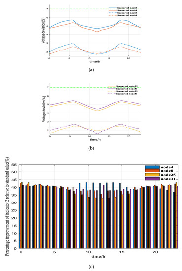
Figure 8.
Voltage deviation curve. (a) Comparison of sub-scenarios of nodes 4 and 8. (b) Comparison of sub-scenarios of nodes 25 and 31. (c) Percentage improvement of voltage deviation relative to standard value.
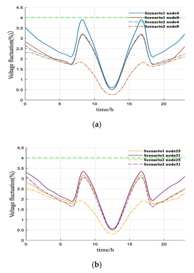

Figure 9.
Voltage fluctuation curve. (a) Comparison of sub-scenarios of nodes 4 and 8. (b) Comparison of sub-scenarios of nodes 25 and 31. (c) Percentage improvement of voltage fluctuation relative to standard value.
According to the GB/T14549 standard, the total current distortion rate of the electric heat storage heating equipment after being connected to the distribution network should be less than or equal to 2.2% [21,32]. Figure 7a,b are the comparison curves of the total distortion rate of the node current harmonics in the two scenarios, and Figure 7c is the percentage increase of the harmonic distortion rate of the node current relative to the national standard value. As can be seen from Figure 7a,b, in Scenario 1, nodes 4 and 31 have a high light intensity between 8:00 am and 7:00 pm. Due to the introduction of a large number of power electronic equipment by photovoltaics, the current harmonic distortion rate exceeded the standard. To ensure the stability of the system, wind abandonment, light abandonment, and load shedding must occur. In Scenario 2, the current harmonic distortion rate was successfully reduced below the standard value, and the improvement rates were 45% and 47%, respectively. Although nodes 8 and 25 did not exceed the standard, the percentage of improvement through energy storage optimization can reach up to 50% and 26%. As can be seen from Figure 7c, the percentage of improvement of power quality relative to the standard value at each time was a positive value, which means that the power quality had improved. From 8 am to 7 pm, ETSHE mainly used the abandoned light resources, and other times mainly used abandoned wind resources.
According to GB/T12325, the absolute value of the voltage deviation should be less than or equal to 7% [33]. As can be seen from Figure 8, taking into account the load characteristics and the reasonable planning of the ETSHE, the voltage deviation of each node was significantly reduced and the voltage deviation of the access point at each moment was within the allowed range of the national standard. As can be seen from Figure 8a,b, at 12:00 am, the light intensity was the highest, but the corresponding voltage deviation was the lowest. The voltage deviation was inversely proportional to both wind speed and light intensity. Furthermore, as can be seen from Figure 8c, the percentage of each node′s improvement relative to the standard value was positive, with an average improvement rate of 38%, and the voltage deviation of each node was improved.
According to the GB/T12326-2008 standard, the voltage fluctuation of a 10 kV distribution network should be less than or equal to 4% [23]. As can be seen from Figure 9a,b, through the optimized configuration of energy storage, the node voltage fluctuation was improved. At 12:00 am every day, the light intensity was the highest, but the voltage fluctuation is the lowest. It can be seen from Figure 9c that at the time when there was more wind power and photovoltaic power generation, the voltage fluctuation was greatly improved relative to the standard value. Among them, node 4 increased by 23% on average, nodes 8 and 25 increased by about 25%, and node 31 increased by 11.2% on average.
5.4. IEEE-118 System Simulation Analysis
1. Basic data
The standard IEEE-118 distribution system was adopted for simulation analysis [34]. The distribution network contained 19 distributed photovoltaics with a capacity of 0.5 MW, which were connected to nodes 7, 9, 14, 31, 35, 36, 52, 54, 59, 60, 63, 78, 85, 87, 95, 96, 113, 114, and 117. The distribution network also contained 10 distributed wind power generation with a capacity of 0.5 MW, which were connected to nodes 4, 18, 25, 26, 28, 30, 32, 40, 41, and 42. The rest of the data is consistent with the IEEE-33 system, which is not repeated here.
2. Results analysis
(1) Optimal scheduling results of ETSHE considering the load characteristics
The same method was used for node sensitivity analysis, and the set of nodes that were selected to obtain the energy storage access included {3, 6, 10, 35, 38, 44, 47, 48, 61, 66, 77, 78, 79, 91, 92, 93, 114, 115, 117}, a total of 19 nodes. In order to highlight the impact of load characteristics on the planning settings, it was considered that nodes 3, 6, 10, 61, 66, 77, 91, 92, and 93 were residential loads; nodes 35, 38, 78, and 79 were commercial loads; nodes 44, 47, 48 were industrial loads; and nodes 114, 117, and 119 were educational loads.
According to the optimization model constructed in this paper, the IMOPSO algorithm was used to solve the calculation example. The installation position and capacity of the electric regenerative heating equipment are shown in Table 6.
Table 6.
Optimized configuration results.
(2) Node sensitivity analysis before and after comparison
This system is more complex than IEEE-33, so it takes a longer time to calculate. The comparative analysis before and after the node sensitivity analysis is shown in Table 7.
Table 7.
Comparison analysis before and after node sensitivity analysis.
(3) Power quality improvement analysis
From the above simulation results, it can be seen that the power quality of residential and educational loads was similarly affected by new energy generation, while commercial and industrial loads were similar. Therefore, the residential and industrial loads were selected to give the results for node 3 and node 44, respectively.
It can be seen from the simulation results that although the IEEE-118 system had a long and complex calculation time, the node sensitivity calculation could obtain a set of candidate nodes in advance, which improved the efficiency and accuracy of the solution. The same results as those of the IEEE-33 nodes’ power distribution system can be seen in Figure 10, Figure 11, Figure 12, Figure 13, Figure 14 and Figure 15. Through the simulation analysis of the above IEEE-33 and IEEE-118 systems, by configuring a certain capacity of ETHSE at specific nodes of the distribution network, it can not only solve the voltage deviations and voltage fluctuations caused by the photovoltaic and wind power, but can also restrain harmonics, which can improve the power quality of distribution network effectively. Finally, it can be seen that the evaluation levels were all above five levels by using the data envelope analysis method, which indicates that the access scheme is feasible and that the indicators of the access point can reach the prescribed standards. For specific evaluation methods and evaluation levels, see Appendix A.
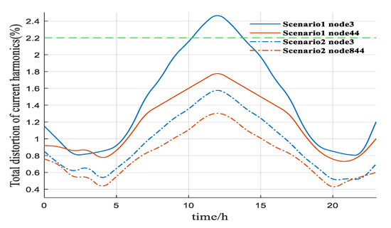
Figure 10.
Current harmonic distortion rate curve.
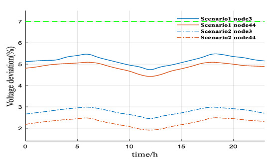
Figure 11.
Voltage deviation curve.
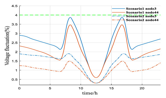
Figure 12.
Voltage fluctuation curve.
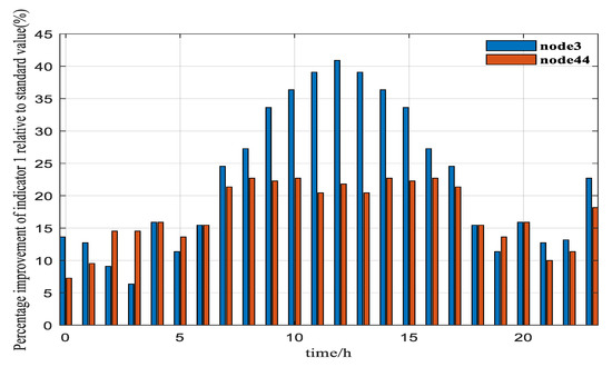
Figure 13.
Percentage improvement of current harmonic distortion rate relative to the standard value.

Figure 14.
Percentage improvement of voltage deviation relative to the standard value.
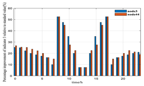
Figure 15.
Percentage improvement of voltage fluctuation relative to the standard value.
6. Conclusions
Aiming at the power quality problems caused by high-permeability distributed photovoltaic and wind power connected to the grid, this paper proposed a method for selecting and determining the capacity of the ETSHE connected to the distribution network, which considered the load characteristics and power quality management. A load forecasting method based on load profile technology was proposed, and the node sensitivity analysis method was used to accurately and quickly solve the multi-objective optimization model, which realized the management of power quality problems such as node voltage overrun, voltage fluctuation, and harmonic pollution. Moreover, the method satisfied the high demand for penetration of photovoltaic and wind power into the distribution network. The main innovations of the work are: (a) comprehensively considering the impact of demand-side response and power quality issues on distribution network planning, and establishing an optimization model that includes power quality indicators and economic indicators; (b) based on the node sensitivity analysis method, so that it can be applied to complex power distribution systems; and (c) the heat load portrait technology is defined to provide a data basis for subsequent optimization. It can provide references for the promotion and application of distributed photovoltaic and wind power, and provide solutions for power quality management methods caused by high-power density distributed energy grid-connection. The next work will consider multiple types of energy storage equipment to further optimize the economy and safety.
Author Contributions
X.-R.L. conceived the idea for the manuscript and wrote the manuscript with input from F.-J.Z., Q.-Y.S., and P.J. All authors have read and agreed to the published version of the manuscript.
Funding
This work was supported by National Key R&D Program of China under grant (2018YFA0702200), the Fundamental Research Funds for the Central Universities (N2004013).
Conflicts of Interest
The authors declare no conflicts of interest.
Abbreviations
| ETSHE | Electric Thermal Storage Heating Equipment |
| DEA | Data Envelopment Analysis |
| FCM | Fuzzy C-means |
| J | Value function of FCM |
| m | Membership factor |
| K | Number of clustering |
| U | Membership matrix |
| C | Cluster center |
| External wind speed value [m/s] | |
| Equivalent temperature of wind speed cooling [°C] | |
| Wind speed correction coefficients | |
| External light value | |
| Light conversion coefficient [] | |
| Total current harmonic distortion | |
| Root mean square value of the fundamental current [A] | |
| Root mean square value of the -th harmonic current [A] | |
| Voltage of node at time [V] | |
| System standard voltage [V] | |
| Current change caused by the output power change [A] | |
| Equivalent impedance of the two-port network distribution network [Ω] | |
| Unit price corresponding to the unit heat supply of the electric boiler [¥/kWh] | |
| Rated heat supply of the electric boiler [kWh] | |
| Unit price of the heat regenerator [¥] | |
| Volume of the heat accumulator [m3] | |
| The increased equipment investment for each additional unit of the rated flow [¥] | |
| Safety factor when calculating the rated flow | |
| Conversion constant of kilowatt hours and joules | |
| Specific heat of the heat medium [J/(kg°C)] | |
| Density of the heat medium [kg/m3] | |
| Difference in heat storage temperature [°C] | |
| The investment cost of the control device for each additional 1kW of the rated heating capacity of the electric boiler [¥] | |
| Equipment installation cost coefficient | |
| Normalized weight coefficient | |
| Active power of node [kW] | |
| Reactive power of node [KVar] | |
| Voltage amplitudes of node [V] | |
| Voltage amplitudes of node [V] | |
| Conductance of branch [S] | |
| Susceptance of branch [S] | |
| Voltage phase angle difference between -th and -th node | |
| Heat provided by the heat storage body to the user during time [kWh] | |
| Maximum design daily heat load [kW] | |
| The ratio of heat load to maximum value in period t of design day | |
| Heat stored in the heat storage body at the beginning of time t [kWh] | |
| Sensitivity coefficient | |
| Relative production efficiency | |
| Weight of the -th power quality indicator | |
| Weight of the -th quality level | |
| -th power quality input indicator in the -th DMU | |
| -th quality level output in the -th DMU indicator |
Appendix A
- Comprehensive evaluation method of power quality based on data envelope analysis
DEA is a comprehensive evaluation method for evaluating the relative efficiency of the same type of multi-index inputs and multi-index outputs [35]. In this method, the weights of the input and output variables are determined from the actual data of each decision unit, and the evaluation is performed from the perspective of the most favorable for the decision unit, which can avoid the influence of subjective factors. Additionally, it is not necessary to determine the display expressions of input and output, which simplifies the internalized relationship between input indicators and output indicators. In the case where the relationship between input indicators and output indicators is complex and difficult to determine, it can reflect its obvious advantages. The data envelopment analysis method was used to evaluate the power quality of each access point, and the access plan was evaluated for power quality at the planning stage, and finally, an ETSHE access plan with a good power quality level was obtained. The basic model and simplified transformation of DEA are as follows:
(1) Model
The model is the most basic DEA model. Suppose there are evaluation objects, each Decision Making Units (DMU) has types of input indicators and types of output indicators. Construct the following model [35]:
where is the relative production efficiency; is the weight of the -th power quality indicator ( = 1,2, …, ); indicates the weight of the -th quality level (= 1,2, …, ); indicates the -th power quality input indicator in the -th DMU; and indicates the -th quality level output in the -th DMU indicator ( = 1,2, …, ). Choose a reasonable input weight vector and output weight vector so that . When = 1, the -th DMU is considered to be the most effective.
(2) Charnes–Cooper transformation
Due to the difficulty of solving the model, the fractional programming is transformed into an equivalent linear programming problem using the Charnes–Cooper transformation, and the dual model is obtained using dual theory.
Carry out the Charnes–Cooper transformation on Equation (A2), and obtain a model in the form of equivalent linear programming as in Equation (A3):
where and represent the “input” and “output” of the -th DMU, respectively. In order to solve in a larger feasible region, and are the relaxation variables. represents the weight of . is the efficiency value of the -th DMU. Generally take = 10−7 in practice. = (1,1,…,1) is used to adjust the relaxation variable.
- Power quality evaluation of the ETSHE planning scheme
The power quality evaluation is carried out for the planning scheme of the ETSHE to be connected to the distribution network. First, the classification of grades should be carried out. There are many ways of classification, among which domestic literatures are mainly divided into grades 3, 5, 7, 9, and 10. This paper divided the power quality indicators into five grades. The assessment level was , which decreased from 1–5 in order: high quality, good, average, qualified, and unqualified.
Considering the influence of the ETSHE connected to the distribution network, the evaluation indicators selected here were the total current harmonic distortion rate, voltage deviation, and voltage fluctuation. 1, 2, and 3 represent the evaluation indicators, respectively. According to the GB/T14549 standard, the total current distortion rate of ETSHE, after it is connected to the distribution network, should be less than or equal to 2.2% [21,32]. According to the standard of GB/T12326-2008, the voltage fluctuation of the 10 kV distribution network should be less than or equal to 4% [23]. According to GB/T12325, the absolute value of the voltage deviation is less than or equal to 7% [33]. According to the national standard, the upper limit is equally divided into grade intervals, and the specific grade standards are shown in Table A1.
Table A1.
Classification of power quality indicators.
Table A1.
Classification of power quality indicators.
| Evaluation Level | Evaluation Indicators | ||
|---|---|---|---|
| X1 | X2 | X3 | |
| Q1 | [0,0.55%] | [0,1.75%] | [0,1%] |
| Q2 | [0.55%,1.1%] | [1.75%,3.5%] | [1%,2%] |
| Q3 | [1.1%,1.65%] | [3.5%,5.25%] | [2%,3%] |
| Q4 | [1.65%,2.2%] | [5.25%,7%] | [3%,4%] |
| Q5 | [2.2%,30%] | [7%,30%] | [4%,30%] |
In this paper, the data envelopment analysis method was used to evaluate the power quality, with 1, 2, and 3 as the inputs and the evaluation level as the output to establish a DMU. The DMU format was (1, 2, 3, ). The median and evaluation level of each level interval in Table 6 were taken as a single decision unit. The data of the standard decision unit of the classification are shown in Table A2. The power quality index grade standard in Table 6 and the DMU of the hierarchical standard in Table A2 were used as the total decision unit to perform the data envelope validity analysis.
Table A2.
Hierarchical decision-making units.
Table A2.
Hierarchical decision-making units.
| DMU | Input Indicator | Output Indicators | ||
|---|---|---|---|---|
| X1 | X2 | X3 | Q | |
| DMU1 | 0.275% | 0.875% | 0.5% | 1 |
| DMU2 | 0.825% | 2.625% | 1.5% | 2 |
| DMU3 | 1.375% | 4.375% | 2.5% | 3 |
| DMU4 | 1.825% | 6.125% | 3.5% | 4 |
| DMU5 | 16.1% | 18.5% | 4.5% | 5 |
Calculate the quality indicators of the access node according to the formula and the average of each indicator. According to the calculation formulas of the total current harmonic distortion rate, voltage deviation, voltage fluctuation, the quality indicators of the power quality of the access node on that day were calculated, respectively, and the average values of the indicators were calculated, as shown in Table A3.
Table A3.
Data of various indicators of power quality.
Table A3.
Data of various indicators of power quality.
| Access Point | Power Quality Index | ||
|---|---|---|---|
| X1 | X2 | X3 | |
| 4 | 3.340% | 2.075% | 0.118% |
| 8 | 4.008% | 4.753% | 0.198% |
| 13 | 4.359% | 5.191% | 0.215% |
| 25 | 5.200% | 2.054% | 0.208% |
| 31 | 5.391% | 2.258% | 0.247% |
As the efficiency value of the power quality indicators of each access point relative to each level was different from the decision unit, it was recorded as , and the level with the smallest absolute value of was used as the evaluation level. Table A4 shows the power quality evaluation results of each access point calculated by the data envelope analysis method.
Table A4.
Proximity of comprehensive efficiency of each decision unit and standard unit.
Table A4.
Proximity of comprehensive efficiency of each decision unit and standard unit.
| Access Point | Evaluation Level | |||||
|---|---|---|---|---|---|---|
| 4 | −0.581 | −0.248 | −0.181 | −0.152 | 0.183 | 4 |
| 8 | −0.462 | −0.129 | −0.062 | −0.033 | 0.302 | 4 |
| 13 | −0.258 | 0.075 | 0.142 | 0.171 | 0.506 | 2 |
| 25 | −0.05 | 0.283 | 0.35 | 0.379 | 0.714 | 1 |
| 31 | 0 | 0.333 | 0.4 | 0.429 | 0.794 | 1 |
As can be seen from the result of the power quality evaluation of each access point by the data envelope analysis method, only the power quality evaluation level of access points 4 and 8 was a level 4 deviation. The level of access point 13 was level 2, and the power quality evaluation level of the access points at 25 and 31 was a quality of level 1. The evaluation level without access points was a level 5 failure, indicating that the access scheme is feasible and that all indicators of the access point can meet the requirements of the standard.
References
- Bracco, S.; Delfino, F.; Pampararo, F.; Robba, M.; Rossi, M. A dynamic optimization-based architecture for polygeneration microgrids with trigeneration, renewables, storage systems and electrical vehicles. Energy Convers. Manag. 2015, 96, 511–520. [Google Scholar] [CrossRef]
- Chathurangi, D.; Jayatunga, U.; Rathnayake, M. Potential power quality impacts on LV distribution networks with high penetration levels of solar PV. In Proceedings of the International Conference on Harmonics and Quality of Power (ICHQP), Ljubljana, Slovenia, 13–16 May 2018; Volume 8, pp. 1–6. [Google Scholar]
- Chai, Y.; Li, G.; Wang, C. Network partition and voltage coordination control for distribution networks with high penetration of distributed PV units. IEEE Trans. Power Syst. 2018, 33, 3396–3407. [Google Scholar] [CrossRef]
- Jin, M.; Feng, W.; Liu, P.; Marnay, C.; Spanos, C. MOD-DR: Microgrid optimal dispatch with demand response. Appl. Energy 2017, 187, 758–776. [Google Scholar] [CrossRef]
- Mokgonyana, L.; Zhang, J.; Li, H. Optimal location and capacity planning for distributed generation with independent power production and self-generation. Appl Energy 2017, 188, 140–150. [Google Scholar] [CrossRef]
- Xiao, J.; Zhang, Z.; Liang, H. Optimization method for location and capacity of public energy storage in distribution network. Autom. Electr. Power Syst. 2015, 19, 60–66 + 73. [Google Scholar]
- Cui, Y.; Liu, W.; Tang, Y. Optimal capacity allocation method for energy storage batteries to improve the voltage level of photovoltaic high-permeability distribution networks. J. Solar Energy 2017, 38, 1157–1165. [Google Scholar]
- Bracco, S. An optimization model for polygeneration microgrids with renewables, electrical and thermal storage: Application to the savona campus. In Proceedings of the 2018 IEEE International Conference on Environment and Electrical Engineering and 2018 IEEE Industrial and Commercial Power Systems Europe (EEEIC/I&CPS Europe), Palermo, Italy, 12–15 June 2018; Volume 5, pp. 1–6. [Google Scholar]
- Brignone, M.; Federico, D.; Francesco, D.; Fossa, M.; Pampararo, F. Modelling and simulating a thermal storage system for the Savona campus smart polygeneration micro grid. Model. Meas. Control C 2018, 79, 83–89. [Google Scholar] [CrossRef]
- Delfino, F. Identification and optimal control of an electrical storage system for microgrids with renewables. Sustain. Energy Grids Netw. 2019, 17, 100183. [Google Scholar] [CrossRef]
- Ghofrani, M.; Arabali, A.; Etezadi-Amoli, M.; Fadali, M.S. A Framework for Optimal Placement of Energy Storage Units within a Power System with High Wind Penetration. IEEE Trans. Sustain. Energy 2013, 4, 434–442. [Google Scholar] [CrossRef]
- Xie, X.; Wang, K.; Liu, Q. A method for location and capacity planning of distributed power sources considering harmonics. J. Wuhan Univ. 2019, 52, 1671–8844. [Google Scholar]
- Chen, C.; Jin, Y.; Cai, Z. Node sensitivity analysis method for power quality management of high-density distributed photovoltaic access distribution network. Power Capacit. React. Compens. 2019, 3, 137–142. [Google Scholar]
- Rahman, S.; Hazim, O. A generalized knowledge-based short-term load-forecasting technique. IEEE Trans. Power Syst. 1993, 8, 508–514. [Google Scholar] [CrossRef]
- Krinidis, S.; Chatzis, V. A robust fuzzy local information c-means clustering algorithm. IEEE Trans. Image Process. 2010, 19, 1328–1337. [Google Scholar] [CrossRef] [PubMed]
- Qin, L.; Zhao, N.; Sun, D.F. Analysis of measured results of heating energy consumption of residential buildings in severe cold areas. J. Northeast Dianli Univ. 2016, 36, 36–40. [Google Scholar]
- Cai, Q. Study on the relationship between meteorological factors and heating load. Dist. Heat. 2016, 4, 27–32. [Google Scholar]
- Seyed, M.S. Electric load forecasting using an artificial neural network. IEEE Trans. Power Syst. 2013, 6, 442–449. [Google Scholar]
- Amjady, N. Short-term hourly load forecasting using time-series modeling with peak load estimation capability. IEEE Trans. Power Syst. 2016, 4, 798–805. [Google Scholar]
- Xu, X.; Zhang, Q.; Mou, Y. Server load prediction algorithm based on CM-MC for cloud systems. J. Syst. Eng. Electron. 2018, 29, 1069–1078. [Google Scholar]
- National Standard of the People’s Republic of China. GBT 24337-2009, Power Harmonics among Public Power Grids; Jointly Issued by General Administration of Quality Supervision, Inspection and Quarantine (GAQSIQ) and Standardization Administration (SAC) of the People’s Republic of China: Beijing, China, 2009.
- Wang, Y.; Wen, W.; Wang, C. Adaptive Voltage Droop Method of Multiterminal VSC-HVDC Systems for DC Voltage Deviation and Power Sharing. IEEE Trans. Power Deliv. 2019, 34, 169–176. [Google Scholar]
- National Standard of the People’s Republic of China. GBT 12326-2008, Voltage Fluctuations and Flickers; Jointly Issued by General Administration of Quality Supervision, Inspection and Quarantine (GAQSIQ) and Standardization Administration (SAC) of the People’s Republic of China: Beijing, China, 2008.
- Cui, Q.; Bai, X.; Dong, W. Collaborative planning of distributed wind power generation and distribution network with large-scale heat pumps. CSEE J. Power Energy Syst. 2019, 5, 335–347. [Google Scholar]
- Barrett, E.; Eustis, C.; Bass, R.B. A Dual-Heat-Pump Residential Heating System for Shaping Electric Utility Load. IEEE Power Energy Technol. Syst. J. 2018, 5, 56–64. [Google Scholar] [CrossRef]
- Zhang, W. Application examples of water heat storage technology for electric boilers. HVAC 2008, 94–97. [Google Scholar]
- Dong, X. Power Flow Analysis Considering Automatic Generation Control for Multi-Area Interconnection Power Networks. IEEE Trans. Ind. Appl. 2017, 53, 5200–5208. [Google Scholar] [CrossRef]
- Christakou, K.; LeBoudec, J.; Paolone, M.; Tomozei, D. Efficient Computation of Sensitivity Coefficients of Node Voltages and Line Currents in Unbalanced Radial Electrical Distribution Networks. IEEE Trans. Smart Grid 2013, 4, 741–750. [Google Scholar] [CrossRef]
- National Standard of the People’s Republic of China. GBT 15543-2008, Power Quality Three-Phase Voltage Unbalance; Jointly Issued by General Administration of Quality Supervision, Inspection and Quarantine (GAQSIQ) and Standardization Administration (SAC) of the People’s Republic of China: Beijing, China, 2008.
- Sato, M.; Fukuyama, Y.; Iizaka, T.; Matsui, T. Total Optimization of Energy Networks in a Smart City by Multi-Swarm Differential Evolutionary Particle Swarm Optimization. IEEE Trans. Sustain. Energy 2019, 10, 2186–2200. [Google Scholar] [CrossRef]
- Duan, H.; Li, P.; Yu, Y. A predator-prey particle swarm optimization approach to multiple UCAV air combat modeled by dynamic game theory. IEEE/CAA J. Autom. Sin. 2015, 2, 11–18. [Google Scholar]
- National Standard of the People’s Republic of China. GBT 29319-2012, Technical Regulations for Access to Distribution Networks of Photovoltaic Power Generation Systems; Jointly Issued by General Administration of Quality Supervision, Inspection and Quarantine (GAQSIQ) and Standardization Administration (SAC) of the People’s Republic of China: Beijing, China, 2012.
- National Standard of the People’s Republic of China. GBT 12325-2008, Power Quality Voltage Deviation; Jointly Issued by General Administration of Quality Supervision, Inspection and Quarantine (GAQSIQ) and Standardization Administration (SAC) of the People’s Republic of China: Beijing, China, 2008.
- Nourizadeh, S.; Karimi, M.J.; Ranjbar, A.M. Power system stability assessment during restoration based on a wide area measurement system. Gener. Trans. Distrib. 2012, 6, 1171–1179. [Google Scholar] [CrossRef]
- Matin, R.K.; Ghahfarokhi, M.I. A two-phase modified slack-based measure approach for efficiency measurement and target setting in data envelopment analysis with negative data. IMA J. Manag. Math. 2015, 26, 83–98. [Google Scholar] [CrossRef]


© 2020 by the authors. Licensee MDPI, Basel, Switzerland. This article is an open access article distributed under the terms and conditions of the Creative Commons Attribution (CC BY) license (http://creativecommons.org/licenses/by/4.0/).