Abstract
Unmanned surface vehicles (USVs) as unmanned intelligent devices can replace humans to perform missions more efficiently and safely in dangerous areas. However, due to the complex navigation environment and special mission requirements, USVs face many challenges in emergency response missions for marine oil spill accidents. To solve these challenges in the emergency response mission of the ‘Sanchi’ oil tanker collision and explosion accident, we designed and deployed an USV to perform the missions of real-time scanning and water sampling in the shipwreck waters. Compared with the previous USVs, our USV owned the following characteristics: Firstly, the improved navigation control algorithms (path following and collision avoidance) can provide high navigation accuracy while ensuring navigation safety; Secondly, an improved launch and recovery system (LARS) enabled the USV to be quickly deployed and recovered in the mission area; Thirdly, a new sampling system was specially designed for the USV. Our USV completed the missions successfully, not only providing a lot of information for rescuers but also offering a scientific basis for follow-up work.
1. Introduction
On 6 January 2018, the Iranian oil tanker ‘Sanchi’ carrying 111,300 tons of condensate collided with the Hong Kong cargo ship ‘Changfeng Crystal’ in the East China sea, at approximately 160 nautical miles east of Shanghai. After the collision, the ‘Sanchi’ burned violently and exploded on 14 January. The ‘Sanchi’ sank 4 h after the explosion. Three people died and 29 people were missing in the accident, and oil leaked from the ‘Sanchi’ polluted 10 km2 of sea area. After the accident, the State Oceanic Administration of China, the Maritime Search and Rescue Center of China, and the Maritime Search and Rescue Center of Shanghai launched the emergency response mission for the accident. Figure 1 is the scene of the accident.
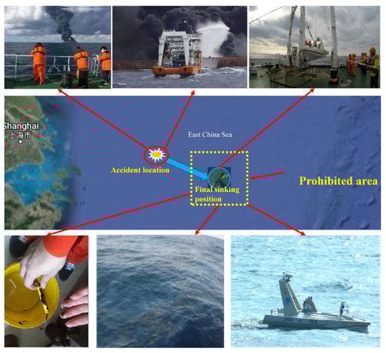
Figure 1.
Accident scene.
In this accident, the ‘Sanchi’ oil tanker carried a total of 113,000 tons of condensate. Condensate is a highly toxic and volatile chemical substance, and there is a risk of deflagration at any time after it leaks. Therefore, it is too dangerous for humans to enter the core area of the accident to perform a mission. We urgently needed a mobile unmanned platform to replace humans in the core area of the accident to obtain the necessary information, such as the submarine topography, the state of the shipwreck, the location of oil spills, and the situation of water pollution.
Unmanned surface vehicles (USVs) are the suitable platform for an emergency response mission. Unmanned meant it could be deployed for a longer time, therefore widening the operational window. Most importantly, the use of the USVs resolved the security challenge of surveying in dangerous areas. In recent years, USVs have been widely researched and applied in a lot of fields [1]. Some new USVs are constantly developed, such as ‘Spartan Scout’ designed by the USV team in San Diego [2], ‘Nighthawk’ from AAC (Accurate Automation Corp) [3], and a range of USVs from ASV(The Company of Autonomous Surface Vechile), such as the USVs that called ‘C-WORKER’ and ‘C-TARGET’ [4]. Although USVs have many applications at this stage, they are limited to carrying out missions for scientific research, such as environmental monitoring [5,6,7], environmental sampling [8,9], communication platform [10,11], and harbor protection and patrol [12,13,14,15]. However, emergency response mission for disaster or accident are performed by AUV(Autonomous Underwater Vehicle) or ROV(Remote Operated Vehicle), for example, Kukulya, A.L. et al. developed an AUV-based approach inspired by an existing small, long-range system, called the Tethys Long-Range AUV (LRAUV), in order to support the Arctic Doman Awareness Center (ADAC) for spill preparedness [16]. Valentine, M.M. et al. used remote-controlled vehicles to quantify large animals at five study sites to determine the effects of the spill on deep-water animals [17].The only application of USVs for disaster was responding to Hurricane Wilma. During the rescue mission, the Center for Robot-Assisted Search and Rescue at the University of South Florida used a USV that called ‘AEOS-1’ to inspect docks and seawalls then bridges [18].
In this emergency response mission, we deployed a newly designed USV. Compared with the previous USVs, (1) the improved navigation control algorithms (path following and collision avoidance) can provide high navigation accuracy while ensuring the navigation safety; (2) the improved LARS (Launch And Recovery System) enabled the USV to be quickly deployed and recovered in the mission area; and (3) a new pump sampling system, which is small in size and light in weight, can be installed or removed at any time.
2. USV System Structure
Our USV consisted of the following parts: Hull, control module, locomotion module, navigation module, and mission module. Each of the parts will be discussed in turn. Figure 2 is an overview of the USV’s architecture.
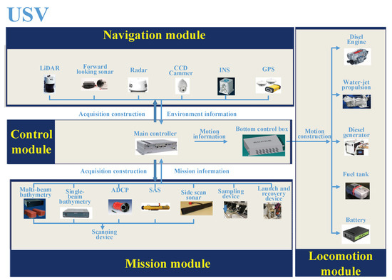
Figure 2.
Unmanned surface vehicle (USV) architecture overview.
2.1. Hull Design
The USV weighed 2300 kg and was 6.28 m × 0.98 m × 0.32 m (length × width × height) with a maximum payload of 1 ton. The hull was divided into three compartments. Forward-looking sonar was installed at the front section. In consideration of vibration problems, an instrument cabinet which elastically connected with the deck was located in the middle section. On the other hand, a circulating cooling system can prevent the instrument cabinet from overheating. Inboard diesel engine, fuel tank, battery, and water-jet propulsion were installed in the tail section. The installation location of each device is shown in Figure 3.
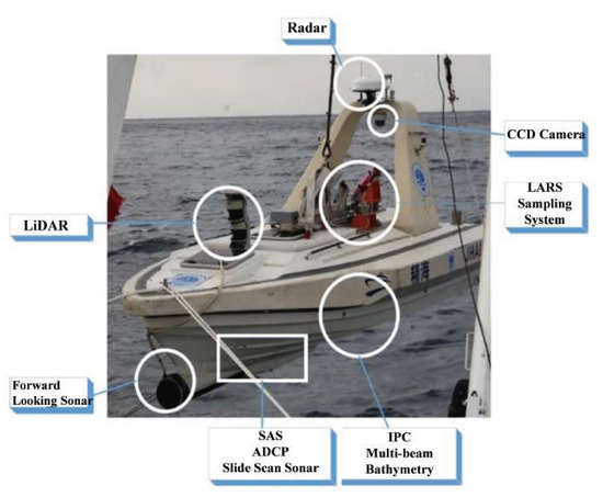
Figure 3.
Device installation location.
2.2. Control Module
The control module can collect sensor information in real-time, control the USV’s movement, manage the mission device, and realize the independent work of the USV. The control module consisted of an industrial personal computer (IPC) and a bottom control box which was equivalent to the brain of the USV. The environmental information, the ontology information, and the target information collected by the sensors were transmitted to the control module. The control algorithms pre-embedded in the IPC processed this information and then different control instructions were calculated and transmitted to other modules.
The key of the control module was the IPC interfaced with a serial extension board (Digital Signal Processor) and a network switch. The general IPC from YanHua’s APAX series was used as a hardware platform and the embedded control system based on Linux was developed. Since data could be collected, processed, and stored independently by the IPC, the loss of the data could be effectively avoided in the case of communication interruption or indirect/incomplete transmission.
2.3. Locomotion Module
The locomotion module was the execution module of our USV. After receiving the control instructions, it drove the USV to perform various actions. Diesel engine, diesel generator, water-jet propeller, fuel tank, and battery constituted the locomotion module. It is worth mentioning that traditional propeller propulsion was replaced by a water-jet propulsion. Better working ability and maneuverability in the shallow water, higher thrust, and lower noise were the obvious advantages of water-jet propulsion technology over propeller propulsion [19,20]. The locomotion module ensured that the maximum speed of the USV was no less than 13 kn(Knot), the cruising speed was about 10 kn, and the ranges of working speed were 4 to 8 kn. The USV could run for about 5 h at cruising speed and 12 h at working speed.
2.4. Navigation Module
The navigation module received data from sensors such as GPS(Global Positioning System), INS(Inertial Navigation System), compass, forward looking sonar, radar, and LiDAR(Light Detection and Ranging), etc. After getting the sensor data, the navigation module analyzed the USV’s position, speed, heading, and obstacle information, and gave the USV’s next speed and heading combined with the mission requirements. If obstacles existed, the speed and heading had to be adjusted through the corresponding collision avoidance algorithm. The architecture of the navigation module is shown in Figure 4.
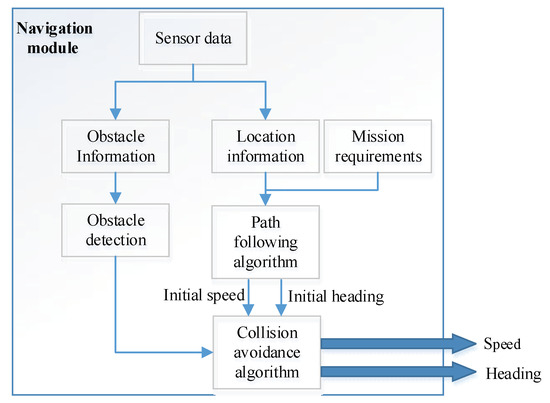
Figure 4.
Navigation module.
2.5. Mission Module
The mission module was divided into three systems: Scanning, sampling, and LARS. The scanning system mainly used the device to realize the underwater exploration. The sampling system was designed to collect water samples in real time. LARS was used to deploy and recover the USV in the mission area.
3. Approach
3.1. Path Following Algorithm
A straight path following algorithm based on the predicted position control was adopted in our USV. The core idea of the algorithm was to calculate the (the USV’s predicted lateral offset). If was larger, the angle which made the USV return to the planned path was also greater.
The schematic diagram of the algorithm is shown in Figure 5. We defined some variables, where and represent the course angle and turning angle required for the USV to return to the planned path, and and represent the actual lateral offset and predicted lateral offset, respectively. The calculation formula of is Equation (3). The calculation formula of is Equation (2), where the linear speed and angular speed of the USV were set to and . and are calculated as Equation (1), where and are the distance and angle from the USV to the terminating waypoint, and is the heading angle of the USV. is the angle of the path, which is calculated from the start and end waypoint of the path. and are calculated based on the USV’s state (position, heading angle, the latitude and longitude information to the terminating waypoint, etc.). Parameters and are called time-lag constant and time-lag slope, respectively. The is a saturation function, in order to modify the distance conversion coefficient into a variable form. Therefore, both the real time and smoothness of the USV movement are considered.
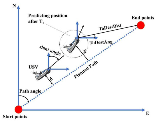
Figure 5.
Path-following algorithm based on predicted position control.
In order to calculate and , , , and are the three parameters that must be calculated, so we focused on how to determine these parameters.
Time-lag constant : Parameter acting on was mainly used to calculate . According to the results of the sea trials, when the USV had a set throttle value of 500, = 5 could make the algorithm achieve a higher control accuracy. When the throttle value increased, the decreased accordingly. Table 1 shows the for each throttle setting.

Table 1.
Selection of for each throttle value.
Time-lag slope : Parameter acting on was related to the sea states during navigation. According to the results of the sea trials, it was appropriate to set the to 5 when the sea states were 1–2. When the sea state was 3, it was appropriate to set the to 5.5 or more. This is because the USV was more difficult to turn in poor sea states, therefore, it was necessary to give a long forecast value when calculating .
Distance conversion coefficient : limits the values of and . This parameter was generally set to 2~3. According to the results of the sea trials, was a suitable value. If set to 3, the maximum control amount of the angle was 60°.
3.2. Collision Avoidance Algorithm
The control of the collision avoidance for USVs is generally divided into two layers [21]. The first layer is global collision avoidance, which is to construct a proper environment model based on the information of known obstacles or danger areas and then plan a safe path. The second layer is the short-range real-time collision avoidance based on the real-time sensor information, which enables USVs to quickly avoid the obstacle that appears suddenly in the surrounding environment. Therefore, short-range real-time collision avoidance is the last line of defense to ensure the safety of USVs.
Velocity obstacle (VO) algorithm is a kind of short-range real-time collision avoidance algorithm commonly used in USVs. However, the traditional VO algorithm does not consider the influence of the kinematic performance of USVs and the error of obstacle movement information, nor does it specify when to start collision avoidance and when to complete. Therefore, in order to overcome these problems, we combined a dynamic window algorithm with elliptic VO algorithm, gave the judgment conditions for when to start and end collision avoidance, and used the virtual obstacle method to reduce the influence of the error of obstacle movement information.
3.2.1. Elliptic VO Algorithm
The basic principle of VO algorithm was introduced in detail in [22], and the key difference between the elliptic VO algorithm and the VO algorithm is the process of solving the tangent. In the VO algorithm, if you want to judge whether a USV will collide with an obstacle, you must require two tangent lines of the obstacle relative to the USV.
As shown in Figure 6, in order to find the tangent lines of elliptical obstacle conveniently, a body-fixed coordinate system and an obstacle coordinate system was established. The is the body-fixed coordinate system of the USV and is the obstacle coordinate system. The red ellipse is an obstacle and the green ellipse is an USV, which was simplified as a particle. Point is the center of the USV. is the center of the obstacle. If the coordinates of the USV in the body-fixed coordinate system are , the coordinates of the USV in the obstacle coordinate system are:
where is the coordinate of the center point of the obstacle in the body-fixed coordinate system and is the rotation matrix.
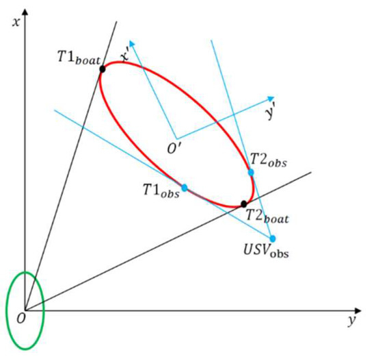
Figure 6.
Ellipse tangents.
When the coordinates of the USV in the obstacle coordinate system are obtained, the tangent coordinate in the obstacle coordinate system can be obtained by Equation (7) ( and in Figure 6):
Then, is converted into the body-fixed coordinate system by using Equation (8):
3.2.2. VO Algorithm Based on Dynamic Window Algorithm
After calculating the colliding VO sets by elliptic VO algorithm, the data in the non-VO sets were the optional collision avoidance velocity vectors for the USV. However, due to the constraint of the dynamic performance of the USV, many velocity vectors in the non-VO sets were inaccessible to the USV. The dynamic window algorithm considered the kinematic performance of the USV [20], and only calculated the moving velocity that the USV can reach within a given time window , that is, the velocity window :
and the angular velocity that can be achieved, that is, the angular velocity window :
In Equation (9), is the current moving speed of the USV and is the acceleration of the USV. In Equation (10), is the current angular velocity of the USV and is the angular acceleration of the USV. According to Equation (11), the heading angle that the USV can get within can be calculated:
where is the current heading of the USV.
Through the Equations (9) and (11), and can be determined, but the elements in sets of and are continuous, which is not conducive to calculation in engineering. Therefore, is discretized into speeds and is discretized into heading directions. Each discretized velocity and heading form a velocity vector , and then there are velocity vectors. The set of velocity vectors is called reachable velocity (RV). The velocity vectors satisfying Equation (9) in the RV set will collide with the obstacle. Excluding these velocity vectors from the RV set can obtain a safe set of velocity vectors, called reachable avoidance velocity (RAV):
As shown in Figure 7, the red area is VO area, the intersection of RV and VO is the velocity vector where collision will occur, and the RAV part is the safe velocity vector.
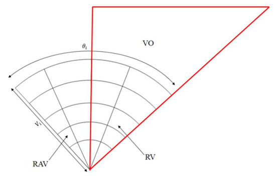
Figure 7.
RV(Reachable Velocity)and RAV (Reachable Avoidance Velocity).
After obtaining the RAV, it was necessary to select the appropriate velocity vector in the RAV according to the mission requirements. In different missions, there are different selection criteria, and the following evaluation formula was used to select in this mission:
where is the current speed of the USV, is the current heading of the USV, is a certain velocity vector in RAV, and , which can maximize , is taken as the velocity vector for the USV to avoid the obstacle. Once a velocity vector is selected, the USV will always travel along this speed vector until there are new dangerous situations or the obstacle is completely avoided.
3.2.3. Starting Collision Avoidance
When judging whether the USV will collide with an obstacle, the distance between the USV and the obstacle is the smallest at the collision time, and their respective positions are called CPA(Close Point Approach). The time required for the USV to reach its CPA point is called . As shown in Figure 8, the red and green solid ellipses are the positions of the obstacle and USV at the time , and are the velocity vectors of the obstacle and USV at time , the red and green dashed ellipses are the positions of the obstacle and USV at time , and the and points are the positions of the center points of the obstacle and USV at time . The is calculated from Equation (14):
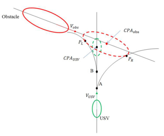
Figure 8.
Close point approach and start avoidance point.
Assuming that the speed of the USV is kept constant, i.e., the USV can turn at a constant angular acceleration. In Figure 8, in the process of sailing to point, the USV turns left with a constant angular acceleration at point , which is tangent to the obstacle at point and just along the path . The time required for the USV to sail from point to point is . Then the USV starts to turn left to avoid the obstacle at the time , which is just tangent to the obstacle at point is calculated from Equation (15):
where , are the coordinates of point and point in the obstacle coordinate system, respectively and are the current velocity, heading, angular velocity, and angular acceleration of the USV, respectively. is the sum of the distances from to the ellipse in the obstacle coordinate system. The is the semimajor axis of the ellipse. The USV turning right is similar to turning left. The time of starting collision avoidance is that can be calculated by Equation (16):
where is a coefficient that is greater than 1 to ensure the safety and smooth turning of the USV. When , the USV starts to avoid the obstacle.
3.2.4. Ending Collision Avoidance
In this algorithm, the USV needs to travel to the destination along the planned path, therefore, collision avoidance can be ended as long as the USV meets the requirements:
In Equation (17), is the velocity vector planned for path following and is the velocity vector when the USV sails to the target point.
3.2.5. Virtual Obstacle
The VO algorithm is set to fully know the obstacle motion information. However, in the actual navigation process, the motion information of the obstacle obtained by the sensor had errors (our USV used LiDAR as the collision avoidance sensor). These errors can cause the USV to collide with the obstacle and, therefore, need to be considered.
Assuming that the velocity vector of the obstacle obtained by the sensor is and the error set of the velocity vector of the obstacle is , the actual velocity vector set of the obstacle is:
where is a Minkowski vector sum operation. Assuming that each element in the is a velocity vector of a virtual obstacle, and the position and size of the virtual obstacle are the same as the original obstacle, the velocity vector of the virtual obstacle is:
Find the VO set of the obstacle and its associated virtual obstacle and this set is the final VO set of the obstacle.
The flowchart of the short-range real-time collision avoidance algorithm is shown in Figure 9.
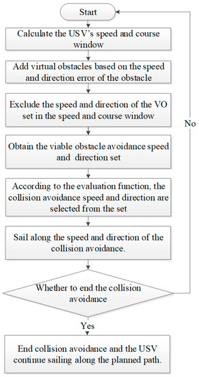
Figure 9.
The flowchart of the short-range real-time collision avoidance algorithm.
3.3. LARS
The mothership carrying out this mission was equipped with a davit type of LARS. Based on this LARS, we developed a special automatic docking device that solved the problems of docking between our USV and the LARS, thereby improving the accuracy and efficiency of deployment and recovery.
Traditional docking devices use a rubber band to eject a rope onto the mothership, and it is necessary to manually reset the rubber band after each ejection, which is cumbersome and dangerous. The use of the rubber band is limited, especially in the environment of high temperature and humidity. Therefore, it has to replace the rubber band frequently, which greatly increases the cost of use. In addition, the elastic force of the rubber band is fixed and the ejection distance is inconvenient to adjust. The newly designed device used an ejection mechanism of the high-pressure gas type instead of the rubber band, which could flexibly change the ejection distance by adjusting the pressure of the compressed air and automatically inflating after each ejection. Compared with the previous ejection mechanism, the new ejection mechanism greatly improved the accuracy, safety, and flexibility of the whole system. The distance of the minimum ejection was 10 m, the distance of the maximum ejection was 100 m, and the inflation time was less than 5 s. The device had both automatic and manual modes. When in the automatic mode, the USV automatically judged the relative position with the mothership, according to the GPS information, adjusted the ejection parameters, and completed ejection. When in the manual mode, the operator can adjust the ejection parameters of the device through the console on the mothership. In practical applications, the device can safely and quickly deploy or recover 3 tons of USV (7.5 m length) under the sea state 4.
As shown in Figure 10, there were three parts in the docking device: (1) The ejection mechanism: The lead and gas cannon were ejected from the USV. (2) The PTZ (Pan/Tilt/Zoom) mechanism: Adjust the launching attitude of the ejection mechanism to ensure that the gas cannon and lead can be launched to the mother ship. The PTZ structure can be adjusted between 0–70° and 0–180° in the pitch and horizontal directions. (3) The docking mechanism: The interface between the USV and the mothership, which realized the lifting of the USV. As shown in Table 2, according to the results of the sea trials, we measured the flying height and time of the gas cannon when the ejection mechanism launched at different initial angles.
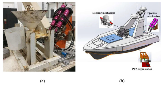
Figure 10.
Docking device (a) Architectural overview of the docking device. (b) Composition of the docking device.
Table 2.
The test results of the ejection mechanism.
We focused on the recovery process because the deployment process was simple and warranted no further discussion. The recovery process is shown in Figure 11 (in the automatic mode). Step (1): The USV sails to the vicinity of the mother ship, and the USV’s GPS information is transmitted to the IPC, which calculates the recovery parameters (gas pressure, PTZ mechanism angle, etc.) based on the relative positions of the USV and mothership. Step (2): Start the ejection mechanism and the lead and gas cannon are ejected to the deck of the mothership. Step (3): Slide the connector on the boom of the mothership into the locking device through the lead. Step (4): When the sensor detects the connector has fully entered the docking mechanism, the docking mechanism quickly locks the connector and then lifts the USV.
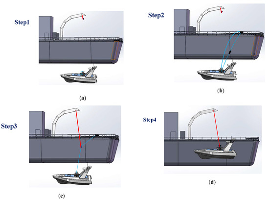
Figure 11.
Flow chart of the recovery process. (a) Step 1. (b) Step 2. (c) Step 3. (d) Step 4.
3.4. Sampling System
We designed a pump sampling system for our USV, which used a high-precision quantitative peristaltic pump to pump water samples by alternately squeezing and releasing the flexible delivery hose. The delivery hose can be placed at different depths to obtain water samples from different layers. Compared with other types of pumps, the quantitative peristaltic pump did not directly contact the water samples and could precisely control the sampling rate. The maximum sampling rate of the system was 1200 mL/min, and the system could flexibly adjust the sampling rate in the range of 500 mL/min–1000 mL/min. The weight of the system was only 10 kg, the system was 0.3 m 0.2 m 0.5 m (length width height) and was directly installed on the deck of the USV, which could be removed at any time. In order to improve the reliability of the system, five independent pump sampling systems were installed on the USV.
As shown in Figure 12, the system was composed of a peristaltic pump, an automatic retracting hose, and a friction wheel. When the USV received the instruction of the sampling, the friction wheel drove the hose into the water, and then the peristaltic pump alternately squeezed and released the flexible delivery hose to pump the fluid into the collecting box. Finally, when the sampling work was completed, the flexible delivery hose was recovered.
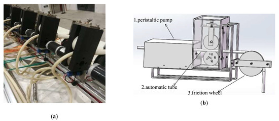
Figure 12.
Sampling system (a) Architectural overview of the sampling system. (b) Composition of the sampling system.
4. Mission
4.1. Mission Plan
In this mission, our USV was required to cover the mission area with minimum cost and obtain the mission data. In order to ensure that the entire shipwreck could be scanned, according to the shape data of the ‘Sanchi’, the direction of the wind, and the flow of the water, we determined a rectangular mission area of 600 600 m based on the GPS information of the sinking position.
According to the mission area, the distribution information of obstacles (mainly the navigation mark of the accident area and the rescue buoys that were urgently placed after the accident) and the scanning width of the USV, the mission area was modeled by the method of the scan-line fill. As shown in Figure 13a, after the environment was modeled, the mission area was decomposed into a series of grids with attribute information, and the USV formed a path that completely covered the environment by successively selecting the next scan grid. Based on the rules of the maritime measurement, the selection principle of the grid node was that of using the method of the global path planning with artificial initial path constraints. Figure 13b is the planned path of the USV for this mission. A total of 9 lines were planned, each line was 440 m, and the distance between the lines was 40 m. It is worth mentioning that when the USV worked according to the planned path, it could replan the mission area according to the relative position of the shipwreck and the USV after finding the shipwreck, thus improving the work efficiency.
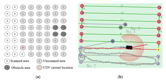
Figure 13.
(a) Environmental modeling. (b) The planned path of the mission.
4.2. Mission Process
On the morning of 15 January 2018, we received orders and boarded on the XianYangHong19 (mothership for our USV) to the accident area. After the mission, the Maritime Search and Rescue Center of Shanghai urgently designated an area with a radius of 10 nautical miles around the sinking position of the ‘Sanchi’. All nonrescue vessels were prohibited from entering this area. Figure 14 shows the specific process of the mission.
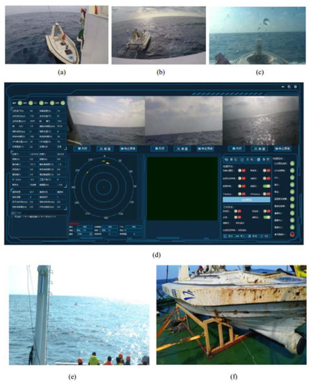
Figure 14.
The USV in the mission: (a) The USV was being deployed in the mission area. (b) The USV was deployed successfully and sailed to the target. (c) The USV was scanning. (d) Display control interface on the mothership. (e) The USV was returning to the mothership. (f) The surface of the hull after the mission was completed.
At 8:20 on 18 January 2018, the USV was successfully deployed at the edge of the mission area. On the day of the mission, the wind speed was 7.8 m/s, the wind direction was 32.5°, the temperature was 9.3 °C, and the wave height was 1.2 m. At 8:30 the USV began to work along the planned paths. At 8:57, the ‘Sanchi’ oil tanker was found from the multibeam images. The images showed that the ‘Sanchi’ oil tanker was located below the starboard of the USV and at the angle of 10° to the USV’s heading. We narrowed the scope of the mission area based on the preliminary scan results and replanned the path on the basis of the previously planned path. Three lines were added to the north direction, at the same time, two north-south direction lines were added. The length of the line was 380 m and the spacing was 270 m. The USV continued to work and then the full-precision multibeam images of the ‘Sanchi’ were obtained at 9:08. After the shipwreck was completely scanned, five sampling points were set up in the horizontal and vertical direction of the shipwreck. The sampling depth was set to 0 m, 0.3 m, 0.5 m, 0.8 m, and 1.0 m and the interval was 10 m. At 10:58, the USV returned to the mothership and then the technicians immediately extracted the water samples and conducted a comprehensive inspection of the USV (Supplementary Materials).
4.3. Mission Data
4.3.1. Path Following
In Figure 15a, the gray straight line indicates the planned path, and the dotted line indicates the actual path of the USV. What we need to explain is that we only focused on the path following error related to the mission, and we did not focus on the path following error during the USV sailing to the mission area and returning to the mothership. As shown in Figure 15b, the maximum following error was 3.2150 m. The following error within 2 m accounts for 97.70%. The data proved that the straight path following algorithm can ensure the USV to have high navigation accuracy in this mission.
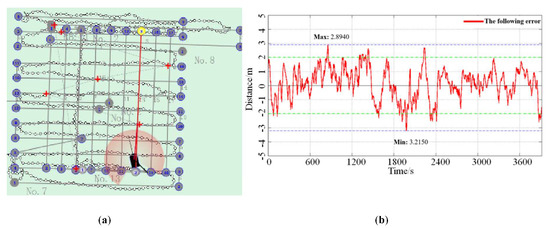
Figure 15.
Path following error of the USV: (a) Path of the USV, (b) changes of the path following error during the mission.
4.3.2. Collision Avoidance
Figure 16a–e shows a complete collision avoidance process of our USV during the mission. As shown in Figure 16a, the USV was sailing normally according to the planned path, and a large rescue vessel was coming from the right side of the USV. As shown in Figure 15b–d, when the USV detected the vessel, the collision avoidance process started, the USV began to change the path according to the collision avoidance parameters, steered to the right, and detoured from the rear side of the vessel until it successfully and safely bypassed the vessel, and then returned to the planned path. Figure 16e shows the change of the path during the whole collision avoidance process.
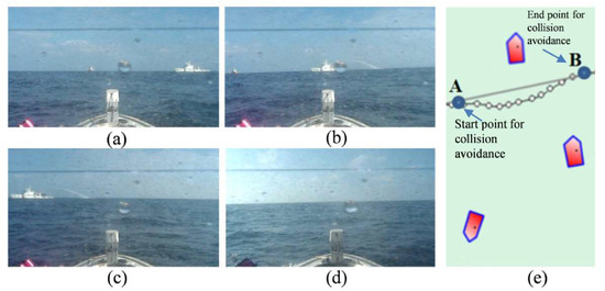
Figure 16.
Process of the collision avoidance: (a) Start collision avoidance, (b,c) collision avoidance, (d) return to the test path after avoiding the obstacle, (e) path in the process of collision avoidance.
Then, we analyzed the changes of the USV’s heading angle and lateral offset during collision avoidance process. As can be seen from Figure 17a,b, during the initial stage, the USV was sailing along the path with an angular direction of 70.219°, while the lateral offset was controlled within 3 m. Starting from 55 s, the USV detected the obstacle and then turned to the right. At this time, the lateral offset started to decrease (the lateral offset was positive on the left side of the path), and, at most, the lateral offset was about −20 m. After completely avoiding the obstacle, the USV began to quickly adjust its path, turn left, and return to the planned path. So the lateral offset gradually increased until it returned to near 0, indicating that the USV returned to the planned path. As shown in Figure 17c, during the whole collision avoidance process, the nearest distance between the USV and the obstacle was 16 m, which is sufficient to ensure navigation safety.
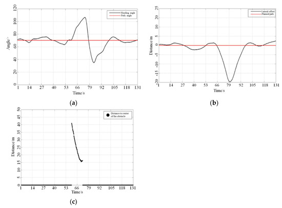
Figure 17.
Collision avoidance results of the USV. (a) Changes in heading angle. (b) Changes in lateral offset. (c) Change in distance between the USV and the obstacle center.
4.3.3. Scan
Figure 18a represents the front view of the shipwreck, where you can see the total length of the shipwreck was 274 m. Figure 18b shows the side view of the shipwreck. We can see that the prominent cockpit was perpendicular to the surface of the seabed, indicating that the shipwreck was also perpendicular to the surface of the seabed.
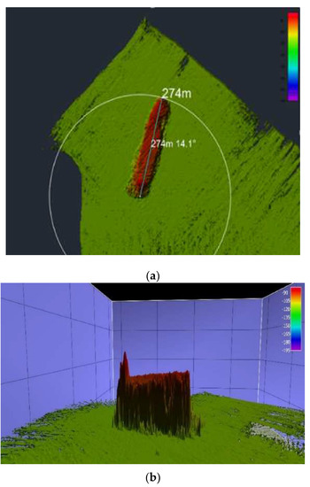
Figure 18.
‘Sanchi’ multibeam view: (a) Shipwreck front view, (b) shipwreck side view.
By preliminary judgment, the oil spill point was located in the position where the hull was hit in the accident. It is well known that a huge impact can cause a partial structural loss of the hull, so the location where the structural loss occurs is the point of the impact. Referring to Figure 19a, we found a gap in the front view. In order to further judge whether the gap was caused by the collision, we took the cross-section 1 at the gap and took another cross-section 2 near the 1, then generated the height change diagram of the two cross-sections. Referring to the Figure 19b,c, we found that the cross-section 1 had a significant drop in height at the same location compared with the cross-section 2, indicating that the cross-section 1 had a structural loss. Combined with the dimensional structure data of the ‘Sanchi’ oil tanker, we confirmed that the gap in Figure 19a was caused by the collision, and the oil spill point was at this gap.
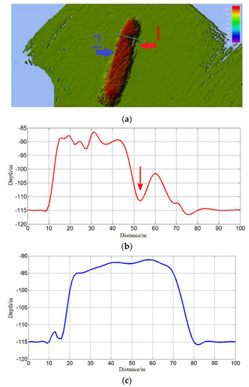
Figure 19.
Cross-sectional view of ‘Sanchi’ multibeam: (a) Cross-section position, (b) height change of cross-sections 1, (c) height change of cross-sections 2.
The multibeam images not only helped us confirm the position and posture of the shipwreck, but also found the position of the impact to confirm the point of the oil spill. On the one hand, this information helped us infer the oil spill rate of the shipwreck and adjust the mission plan in time. On the other hand, it provided strong evidence for future accident investigation.
4.3.4. Water Sampling
Our USV collected a total of 5 bottles of the water samples (2000 mL per bottle) at 5 different locations. After the USV returned to the mothership, the China State Oceanic Administration analyzed the water samples. Figure 20 shows the collected water samples. Since oil can change and destroy the normal ecological balance in the water, serious oil spill accidents often destroy the ecological environment for decades. Therefore, water quality monitoring must be carried out through the mission and operate for a long time after this mission. Even if the oil concentration in the water basically returns to normal, monitoring cannot be stopped until the ecological environment is fully restored.
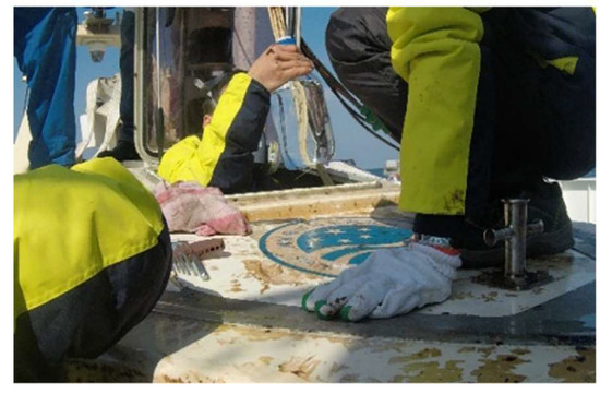
Figure 20.
The water samples.
5. Conclusions
This paper described the application of our USV in the emergency response mission for the ‘Sanchi’ oil tanker collision and explosion accident. The improved algorithms of navigation control, an improved automatic LARS, and a new special sampling system allowed the USV to be quickly deployed to the mission area, and enabled the USV to have higher navigation accuracy and navigation safety in the mission. In this mission, the USV performed the real-time scanning and sampling, which provided important information for determining the exact location of the shipwreck, locating the oil spill point, estimating the amount of oil spilled, salvaging the shipwreck, and evaluating the pollution. The information not only provided a lot of help to rescuers, but also offered a scientific basis for the follow-up work (such as ecological recovery, accident identification, etc.).
Although the USV completed the mission, we also found some new issues in the mission, such as the stability of the USV was insufficient. Especially in poor sea states, the negative impact of the environmental disturbances (winds, waves, and currents, etc.) on the stability was particularly evident. The capability of a single USV was also limited. Due to the limitations of the speed and the payload, a single USV had to take a long time to complete a complex mission. Once the USV breaks down in the process of working, the mission must be suspended.
We will continue to solve the above issues by actively predicting the environmental disturbances’ information and establishing a multiple USVs’ system. Active prediction of the environmental disturbance information for the USVs can calculate the compensation instructions in advance according to environmental disturbances, so that the stability of USVs can be improved. Multiple USVs’ system with the cooperation between the USVs can enhance the USVs’ robustness and reliability, improve mission performance, reduce costs, and provide the best mission policy.
Supplementary Materials
The following are available online at https://www.mdpi.com/2076-3417/10/8/2704/s1, Video: Collision avoidance, Deployment, Recovery.
Author Contributions
H.P., Y.L., J.L., S.X., Y.P. designed USVs; Y.Y. (Yang Yang), X.L., C.Z., J.K., J.C. and D.Q. carried out the missions; Y.L., Z.S., W.S. analyzed mission results. H.P., Y.Y. (Yi Yang), S.G. analyzed sequencing data and developed analysis tools. Y.L. wrote the manuscript. All authors have read and agreed to the published version of the manuscript.
Funding
This work was supported in part by the National Natural Science Foundation of China (9174810194).
Acknowledgments
The authors wish to thank the State Oceanic Administration of China, the Maritime Search and Rescue Center of China, and the Maritime Search and Rescue Center of Shanghai that have helped in the missions.
Conflicts of Interest
The authors declare there is no conflicts of interest regarding the publication of this paper.
Abbreviations
| Unmanned Surface Vehicle | USV |
| launch and recovery system | LARS |
| Autonomous Underwater Vehicle | AUV |
| Remote Operated Vehicle | ROV |
| Knot | kn |
| Global Positioning System | GPS |
| Inertial Navigation System | INS |
| Light Detection and Ranging | LiDAR |
References
- Tiron, R. High-Speed Unmanned Craft Eyed for Surveillance Role. Natl. Def. 2002, 5, 27. [Google Scholar]
- Accurate Automation Corporation. Available online: https://www.accurateautomation.com/content/Home (accessed on 1 December 2019).
- C-Target3. Available online: https://www.asvglobal.com/product/c-target-3/ (accessed on 5 December 2019).
- Caccia, M.; Bibuli, M.; Bono, R.; Bruzzone, G. Basic navigation, guidance and control of an Unmanned Surface Vehicle. Auton. Robot 2008, 25, 349–365. [Google Scholar] [CrossRef]
- Furfaro, T.C.; Dusek, J.E.; Von Ellenrieder, K.D. Design, Construction, and Initial Testing of an Autonomous Surface Vehicle for Riverine and Coastal Reconnaissance. In Proceedings of the MTS/IEEE International Conference on OCEANS, Biloxi–Marine Technology for the Future: Global and local Challenges, Piscataway, NJ, USA, 26–29 October 2009; pp. 1–6. [Google Scholar]
- Anon. 2014. Available online: http://www.asvglobal.com/ (accessed on 21 August 2015).
- Naeem, W.; Xu, T.; Sutton, R.; Tiano, A. The design of a navigation, guidance, and control system for an unmanned surface vehicle for environmental monitoring. Proc. Inst. Mech. Eng. Part M J. Eng. Marit. Environ. 2008, 222, 67–79. [Google Scholar] [CrossRef]
- Caccia, M.; Bibuli, M.; Bono, R.; Bruzzone, G.; Bruzzone, G.; Spirandelli, E. Unmanned surface vehicle for coastal and protected waters applications: The charlie project. Mar. Technol. Soc. J. 2007, 41, 62–71. [Google Scholar] [CrossRef]
- Caccia, M. Modelling and identification of the Charlie2005 ASC. In Proceedings of the 14th Mediterranean Conference on Control and Automation, Ancona, Italy, 28–30 June 2006; pp. 1–6. [Google Scholar]
- Roberts, G.N.; Sutton, R. (Eds.) Advances in Unmanned Marine Vehicles; The Institution of Engineering and Technology: London, UK, 2006. [Google Scholar]
- Gomes, P.; Silvestre, C.; Pascoal, A.; Cunha, R. A Path-Following Controller for the DELFIMx Autonomous Surface Craft. In Proceedings of the 7th IFAC Manoeuvring and Control of Marine Craft, Lisbon, Portugal, 20–22 September 2006. [Google Scholar]
- Motwani, A. A Survey of Uninhabited Surface Vehicles; MIDAS Technical Report. MIDAS.SMSE.2012.TR.001; Plymouth University: Plymouth, UK, 2012. [Google Scholar]
- Murray, J. Sentry—An Unmanned Swimmer Intercept System. DTIC Document; QinetiQ North America Inc., Woburn Ma Technology Solutions Group: Woburn, MA, USA, 2008. [Google Scholar]
- Sonnenburg, C.R. Modeling, Identification, and Control of an Unmanned Surface Vehicle. Ph.D. Thesis, Virginia Polytechnic Institute and State University, Blacksburg, VA, USA, 2012. [Google Scholar]
- Yang, W.R.; Chen, C.Y.; Hsu, C.M.; Tseng, C.J.; Yang, W.C. Multifunctional inshore survey platform with unmanned surface vehicles. Int. J. Autom. Smart Technol. 2011, 1, 19–25. [Google Scholar] [CrossRef]
- Vasilijevic, A.; Stilinovic, N.; Nad, D.; Mandic, F.; Miskovic, N.; Vukic, Z. AUV Based Mobile Fluorometers: System for Underwater Oil-Spill Detection and Quantification. In Proceedings of the Sensors Applications Symposium, Zadar, Croatia, 13–15 April 2015; pp. 1–6. [Google Scholar]
- Valentine, M.M.; Benfield, M.C. Characterization of epibenthic and demersal megafauna at Mississippi Canyon 252 shortly after the Deepwater Horizon Oil Spill. Mar. Pollut. Bull. 2013, 77, 196–209. [Google Scholar] [CrossRef] [PubMed]
- Murphy, R.R.; Steimle, E.; Griffin, C.; Cullins, C.; Hall, M.; Pratt, K. Cooperative use of unmanned sea surface and micro aerial vehicles at Hurricane Wilma. J. Field Robot. 2008, 25, 164–180. [Google Scholar] [CrossRef]
- Park, W.G.; Jang, J.H.; Chun, H.H.; Kim, M.C. Numerical flow and performance analysis of waterjet flow and performance analysis of water-jet propulsion system. Ocean Eng. 2005, 32, 1740–1761. [Google Scholar] [CrossRef]
- Kim, M.C.; Chun, H.H.; Kim, H.Y.; Park, W.K.; Jung, U.H. Comparison of waterjet performance in tracked vehicles by impeller diameter. Ocean Eng. 2009, 36, 1438–1445. [Google Scholar] [CrossRef]
- Fox, D.; Burgard, W.; Thrun, S. The dynamic window approach to collision avoidance. IEEE Robot. Autom. Mag. 1997, 4, 23–33. [Google Scholar] [CrossRef]
- Fiorini, P. Motion planning in dynamic environments using velocity obstacles. Int. J. Robot. Res. 1998, 17, 760–772. [Google Scholar] [CrossRef]


© 2020 by the authors. Licensee MDPI, Basel, Switzerland. This article is an open access article distributed under the terms and conditions of the Creative Commons Attribution (CC BY) license (http://creativecommons.org/licenses/by/4.0/).