Effect of Displacement Current on the Finite-Difference Modeling of Natural Source Electromagnetic Diffusion

Abstract

For electromagnetic (EM) modeling based on the electric-field formulation at low frequencies, the quasi-static approximation (i.e., only the conduction current is considered and the displacement current is ignored) is commonly applied, and a small conductivity value for the air layer is chosen subjectively. Actually, in the air layer, due to the use of the small conductivity value, the quasi-static approximation is ubiquitously violated. However, the effect of the violation of the quasi-static approximation in the air on EM modeling is not well examined in the literature. In this paper, we investigate this issue by comparing the finite-difference modeling results from the calculation with the quasi-static approximation and those considering both the conduction and displacement currents. For the quasi-static approximation, the conductivity in the air is set to be different small values, and zero air conductivity is used for the modeling with both the conduction and displacement currents considered. Several simple models are designed to verify the numerical solution and study how the assigned conductivity for the air affects the modeling accuracy. One flat model and two models with topography are designed to examine the effect of the quasi-static approximation on the EM modeling results. For frequencies used in typical geophysical applications of EM diffusion, using the quasi-static approximation is able to produce accurate modeling results for models with typical earth conductivity. However, if the rough surface topography is considered, the use of the quasi-static approximation can reduce the EM modeling accuracy substantially at much lower frequencies (as low as several hundred Hz), which is probably due to the inaccurate description of EM waves in the air, and poses problems for applications based on direct EM field interpretation.

1. Introduction

Electromagnetic (EM) methods, such as the magnetotelluric (MT) method, the audio magnetotelluric (AMT) method, and controlled source EM, use the EM diffusion over a wide frequency band range to detect the subsurface geo-electrical structure, from shallow near-surface to great depth [1,2]. It has been widely applied in deep tectonic study, oil and gas detection, mineral exploration, geothermal survey, engineering purposes, and environmental monitoring [3,4,5,6,7].

Forward modeling and inversion are important to understand the subsurface geo-electric structure for the EM survey [8,9]. However, meaningful interpretation of EM data is strongly dependent on the accuracy and efficiency of the forward modeling [10]. The forward problem can be solved numerically with the integral equation, finite-element, and finite-difference methods [11,12]. For models with small scale anomaly, the integral equation method is more efficient and accurate [13]. However, it faces challenges in handling complex structures [13,14]. The differential equation method (e.g., finite-difference and finite-element methods) can be used to model complex structure EM problems efficiently [15,16,17,18,19,20]. Due to the simplicity and efficiency of implementation, the finite-difference method is widely used in the 3D forward modeling [21,22,23,24,25].

In the development of an EM forward modeling algorithm, it is common to apply the quasi-static approximation, where the displacement current is neglected and Maxwell’s equations are simplified [26]. For simulations based on the electric-field formulation, small air conductivity (typically in the range of 10⁻⁴–10⁻¹⁴ S/m) is assigned to avoid ill-conditioning [27,28,29]. This particular choice is sometimes very subjective and its impact on the modeling results is rarely examined. Further, since the use of small conductivity for the air layer is a common practice for EM diffusion modeling based on the electric-field formulation, the displacement current can no longer routinely be neglected at all operating frequencies [27]. This means that the use of the quasi-static approximation in the air can be problematic and deserves further investigation, which is the primary goal of this paper.

In this paper, we investigate the effect of the quasi-static approximation on the finite-difference EM modeling based on the electric-field formulation. This can be realized by comparing the numerical results from modeling based on the quasi-static approximation and considering both the conduction and displacement currents. The investigation is carried out on several synthetic models, with both flat and uneven surfaces, to model the general earth structure.

2. Materials and Methods

2.1. Basic Theory

A time harmonic dependence of e^−wt is assumed for EM fields, and the SI unit system is adopted. In the frequency domain, EM fields in the space are distributed according to Maxwell’s equations:

∇ × E = iωμH,

(1)

∇ × H = (σ-iωε) E.

(2)

where E is the vector electric field, H is the vector magnetic field, ω is the angular frequency, μ is the magnetic permeability, ε is the dielectric constant, and σ is the electrical conductivity. Substituting Equation (1) into Equation (2), we can then get the second order differential equation for electric field E as:

∇ × (∇ × E) − k²E = 0

(3)

with

k² = iωμσ + ω²εμ

(4)

where k is the wavenumber. The first term in Equation (4) accounts for the induction current (imaginary part of k²), and the second term (real part of k²) represents the displacement currents in the medium. In some applications, either the induction part or the displacement part is typically considered, and we refer to the wavenumber including both the induction and displacement terms as the complete wavenumber in this paper for convenience. As indicated in Equation (4), the wavenumber is a function of physical properties of the medium (i.e., magnetic permeability, dielectric constant, and electrical conductivity) and the operating frequency.

The behavior of EM field is dependent on the wavenumber (the loss factor, σ/ωε), in which frequency is typically used as a design parameter, defining different geophysical applications. At low frequencies (typically less than 10⁵ Hz), the wavenumber can be simplified to:

k² = iωμσ,

(5)

where the displacement current is neglected, and only the induction current exists in the medium (namely, the quasi-static approximation). The EM fields are said to be diffusive, as used in MT applications and audio-magnetotelluric (AMT) surveying. At high frequencies (e.g., greater than 10⁵ Hz), the wavenumber can be reduced to:

k² = ω²εμ.

(6)

In such a scenario, the EM field propagates in space without significant attenuation, acting as waves, as used in ground penetrating radar (GPR) applications. However, in real applications, the critical frequency to use in Equation (5) or Equation (6) is usually not known a priori.

In our work, we mainly focus on the geophysical application of the EM diffusion, in which the simplified wavenumber in Equation (5) is routinely applied. For the EM forward modeling based on the electric-field formulation, the air layer needs to be included in the computational domain with conductivities typically set to be small values (e.g., 10⁻⁶–10⁻¹⁴ S/m) and the displacement current is typically ignored. We calculate the loss factor σ/ωε for typical conductivity encountered in geophysical applications, as listed in

Table 1. Loss factors σ/ωε for different operating frequencies and earth conductivities.

f (Hz)	σ (S/m)	σ/ωε	σ (S/m)	σ/ωε
1 × 10−1	1 × 10−2	1.8 × 109	1 × 10−6	1.8 × 105
1 × 100	1 × 10−2	1.8 × 108	1 × 10−6	1.8 × 104
1 × 101	1 × 10−2	1.8 × 107	1 × 10−6	1.8 × 103
1 × 102	1 × 10−2	1.8 × 106	1 × 10−6	1.8 × 102
1 × 103	1 × 10−2	1.8 × 105	1 × 10−6	1.8 × 101
1 × 104	1 × 10−2	1.8 × 104	1 × 10−6	1.8 × 100
1 × 10−1	1 × 10−4	1.8 × 107	1 × 10−8	1.8 × 103
1 × 100	1 × 10−4	1.8 × 106	1 × 10−8	1.8 × 102
1 × 101	1 × 10−4	1.8 × 105	1 × 10−8	1.8 × 101
1 × 102	1 × 10−4	1.8 × 104	1 × 10−8	1.8 × 100
1 × 103	1 × 10−4	1.8 × 103	1 × 10−8	1.8 × 10-1
1 × 104	1 × 10−4	1.8 × 102	1 × 10−8	1.8 × 10-2

. In the earth (normally greater than 10⁻⁴ S/m), the second term of Equation (4) is negligibly small, and EM fields are dominantly diffusive. However, in the air, the conductivity is close to zero, which makes simplification of Equation (4) a problem.

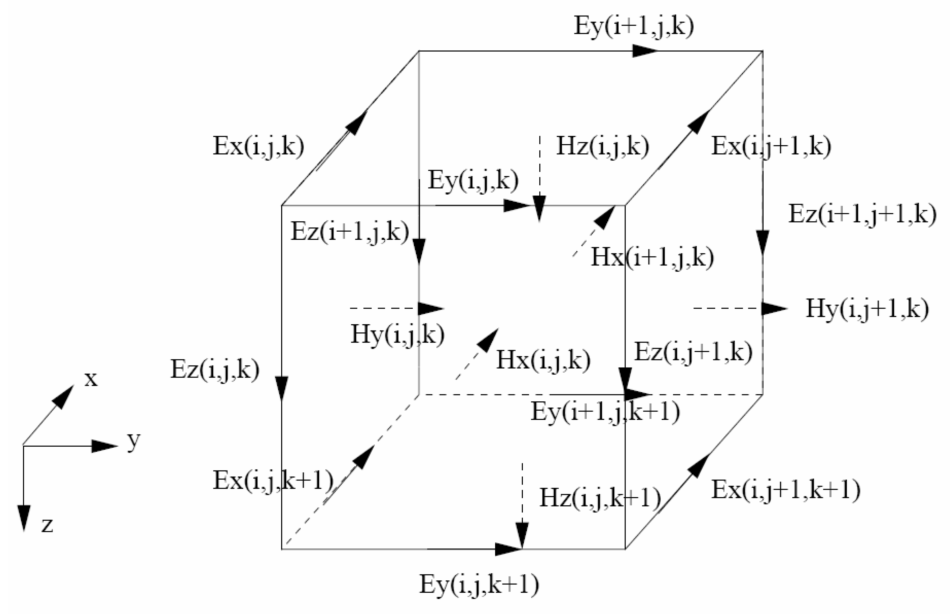
2.2. Finite-Difference Discretization

We apply a finite-difference method to solve Equation (3) on staggered grids (Figure 1). The discretized electric-field components are defined on cell edges and magnetic field components are defined on cell faces [30]. The finite difference discretization for Equation (3) with the complete wave number is similar as that for the static approximation. By applying appropriate boundary conditions, the finite-difference discretization of the Equation (3) results in a linear system:

AE = B

(7)

with

$$A=C^{†}C+diag(i\omega \mu \overline{\sigma }+{\omega }^2\epsilon \mu )$$

(8)

where E is the discretized vector electrical field. Since E is defined on edges, we need to volume average the conductivities of four cells surrounding each edge to get the edge conductivity $\overline{\sigma }$. C is the discrete representation of the curl operator, which maps cell edges to cell faces, and $C^{†}$ is the adjoint of the discrete curl operator, which maps cell faces back to cell edges. B includes the applied boundary condition and source terms for specific EM problems (e.g., for MT only boundary terms are non-zero).

Equation (7) can be solved by either direct or iterative solvers. However, if the size of Equation (7) is significantly large, e.g., for typical MT problems, direct solvers can be prohibitive in terms of both computing time and memory cost, and iterative solvers (such as bi-conjugate gradient (BiCG) used in this paper) are exclusively used. However, the convergence of solving Equation (7) iteratively can be slow due to the abundant null space of the double-curl operator. This problem can be alleviated by the application of preconditioners. As ω becomes very small, such as for long period MT explorations, the numerical solution cannot adequately model the charges accumulated at the discontinuities of conductivity, and this can pose a challenge for iterative solvers to converge. This is commonly improved by enforcing the static divergence correction:

$$\nabla \cdot \sigma E=0.$$

(9)

3. Results

In this section, the impact of the quasi-static approximation on the EM modeling is examined by comparing results from cases treating the air layer differently. For cases based on the quasi-static approximation, different conductivity values are used for the air layer; for the case using the complete wavenumber, zero conductivity for air is used. The code for the quasi-static approximation is implemented in MATLAB based on the work of [30], and its accuracy has been widely tested [10,25]. Since the dielectric constant ε can be considered to be constant in the whole space, the complete wave-number code can be obtained from the quasi-static version by trivially adding a constant to the discretized conductivities. The solver used is the BiCG method preconditioned by Gauss–Seidel. The convergence tolerance for the relative error is set to 10⁻¹⁰. In order to guarantee that each solution is converged, we check the last two iterations to examine their difference (no obvious change is expected). Modeling grids used are designed based on their respective skin depth to guarantee an accurate solution.

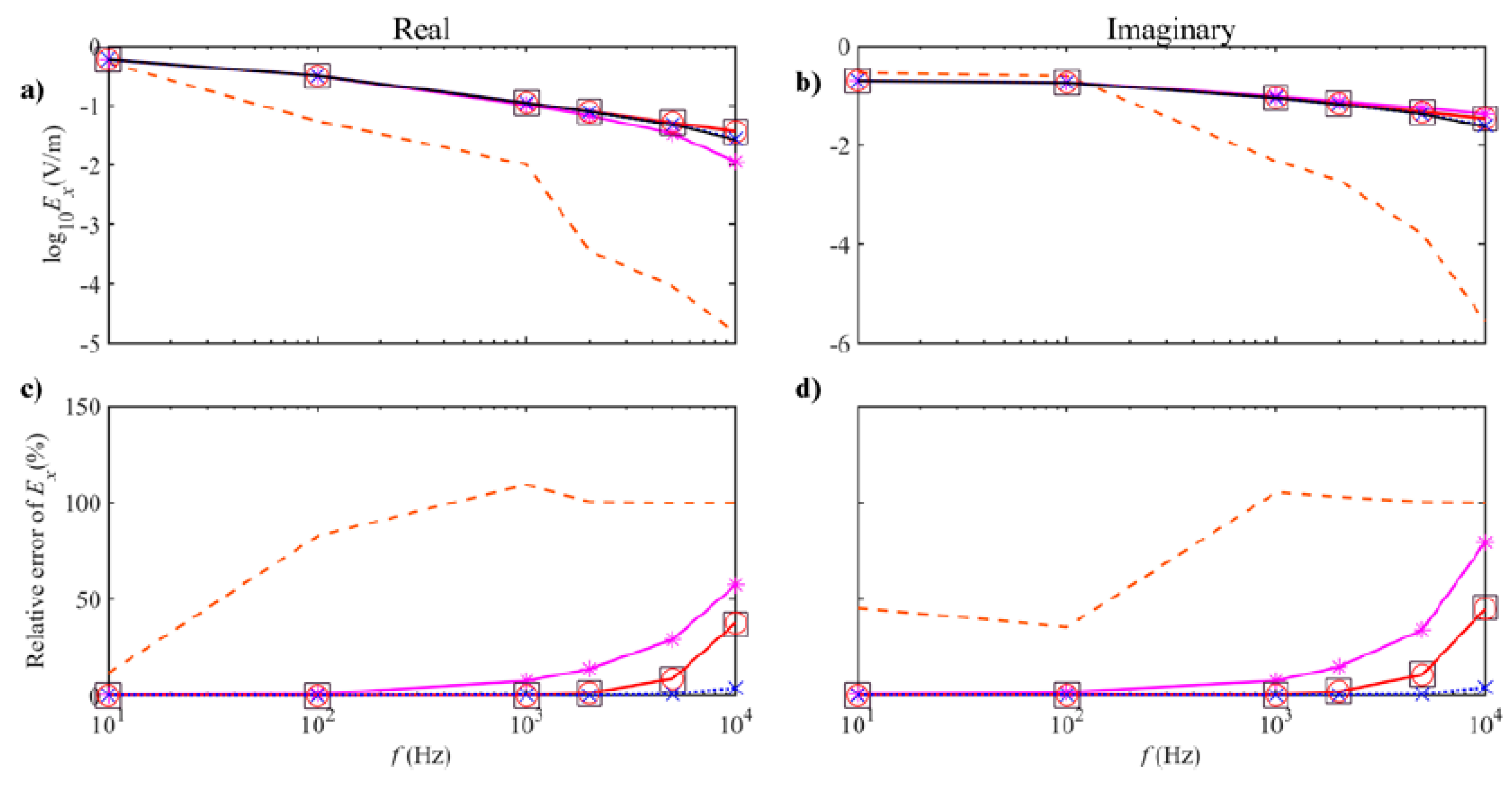
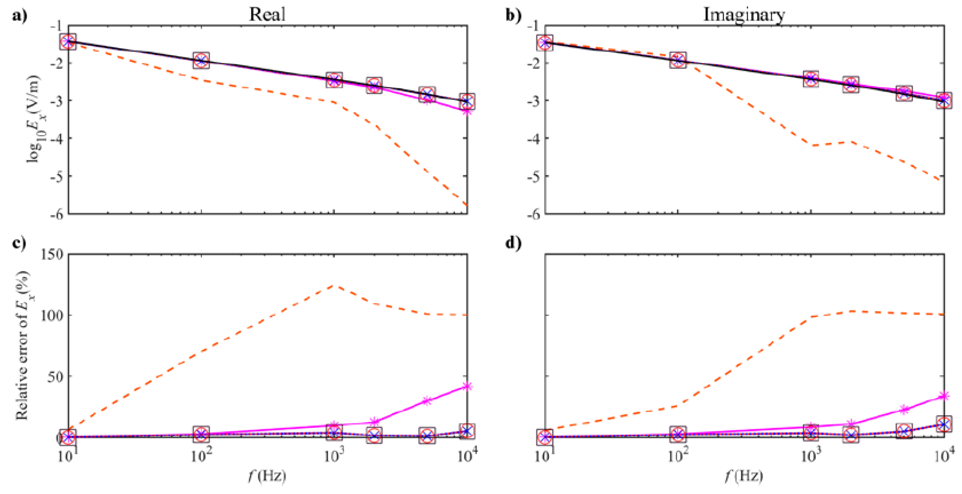
3.1. Simple 1D Models

To examine the effect of the quasi-static approximation on the EM diffusion modeling, we design two half-space models, named model I and model II, respectively. The conductivity is 10⁻⁴ S/m for model I and 10⁻¹ S/m for model II. Six frequencies of 10¹, 10², 10³, 2 × 10³, 5 × 10³, and 10⁴ Hz are considered. For cases based on the quasi-static approximation, the conductivity in the air is set to be 10⁻⁴, 10⁻⁶, 10⁻⁸, or 10⁻¹⁰ S/m. The numerical modeling of electrical responses also using the finite-difference method are compared with the analytical solution [1].

The comparison between the x-component electrical fields calculated by treating air conductivities differently is shown in Figure 2a,b along with the analytical solution for model I. As indicated in Figure 2a,b, the numerical solution for the case using the complete wavenumber matches the analytical solution perfectly. For cases based on the quasi-static approximation, as the conductivity used for the air layer decreases, the differences between the numerical solution and the analytical solution become smaller for both real and imaginary parts of the x-component of the electrical field. Please note that a further decrease in the air conductivity cannot guarantee a better solution as indicated in the figure, called air conductivity saturation here for convenience. For results with the quasi-static approximation, an increase in frequency leads to a larger deviation between the numerical result and the analytical solution. For air conductivity of 10⁻⁸ S/m, while the frequency is less than 10³ Hz, they are generally in good agreement. A more intuitive comparison is indicated in Figure 2c,d, showing similar results as in Figure 2a,b. For cases based on the quasi-static approximation, the relative error of the numerical solution exclusively reaches more than 40% (e.g., real parts have relative errors of 100%, 79%, 45%, and 44% for air conductivity of 10⁻⁴, 10⁻⁶, 10⁻⁸, and 10⁻¹⁰ S/m, respectively) at 10⁴ Hz. Large errors start to appear at frequencies of greater than 10³ Hz for this simple model.

A similar comparison is carried out for model II. The real and imaginary results for the x-component of the electrical field are compared in Figure 3 along with the analytical solutions. The comparison results are generally similar to those indicated for model I. Using the complete wavenumber in the air produces accurate modeling results. For modeling based on the quasi-static approximation, using a conductivity less than or equal to 10⁻⁶ S/m, the numerical results are in good agreement with the analytical solution over the range 10¹–10⁴ Hz.

The two modeling examples above indicate that the quasi-static approximation in the air can affect the accuracy of EM simulation based on the electric-field formulation. The extent of this impact on the modeling results is dependent on the conductivity used for the air and the conductivity of the earth, as well as the operating frequency. For a particular earth conductivity, saturation air conductivity exists. The value of saturation air conductivity is closely related to the earth conductivity (around four orders of magnitude more conductive). When saturation air conductivities are used, the frequency at which the modeling results start to be apparently affected by the quasi-static approximation decreases with decreasing conductivity of the earth.

3.2. 3D Flat Model

The 3D flat model considered is modified from the COMMEMI 3D-2 test model, as shown in Figure 4. Frequencies used in these simulations are 10³, 2 × 10³, and 5 × 10³ Hz. The model domain is discretized with a 60 × 60 × 58 cell mesh (including eight air layers) with the smallest cell size 100 × 100 × 50 m³. A finer discretization and an addition of more air layers does not improve the solution further (to avoid errors caused by the numerical discretization). Since the background conductivity can be considered as 10⁻⁴ S/m, we use conductivity of 10⁻⁸ S/m for the air for the quasi-static approximation case. We compare modeling results for cases using the complete wavenumber (zero conductivity in the air) and using the quasi-static approximation. Modeling grids are the same for the two situations, but can be different for different frequencies.

The comparison between solutions by treating the air conductivity value as constant (i.e., 10⁻⁸ S/m) and those using the complete wavenumber is shown in Figure 5 for different frequencies. The relative errors with respect to the solution based on the use of the complete wavenumber are also calculated. As shown in Figure 5 a–d, at a frequency of 10³ Hz, the modeling results for both real and imaginary parts of the x-component electrical field based on the use of the quasi-static approximation and the complete wavenumber are in good agreement. As the frequency increases, the deviation between them becomes larger. At a frequency of 2 × 10³ Hz, the relative errors for both the real and imaginary parts are exclusively greater than 1%. When the frequency reaches 5 × 10³ Hz, all the relative errors increase to greater than 7% and greater than 9% for the real and imaginary parts, respectively.

The results for the flat model are very similar to those for model I. It can be expected that the frequency at which the quasi-static approximation can produce accurate EM modeling results can be different for different overall earth conductivities. For typical conductivities (greater than 10⁻⁴ S/m), the quasi-static approximation can be valid for frequencies greater than 2 × 10³ Hz.

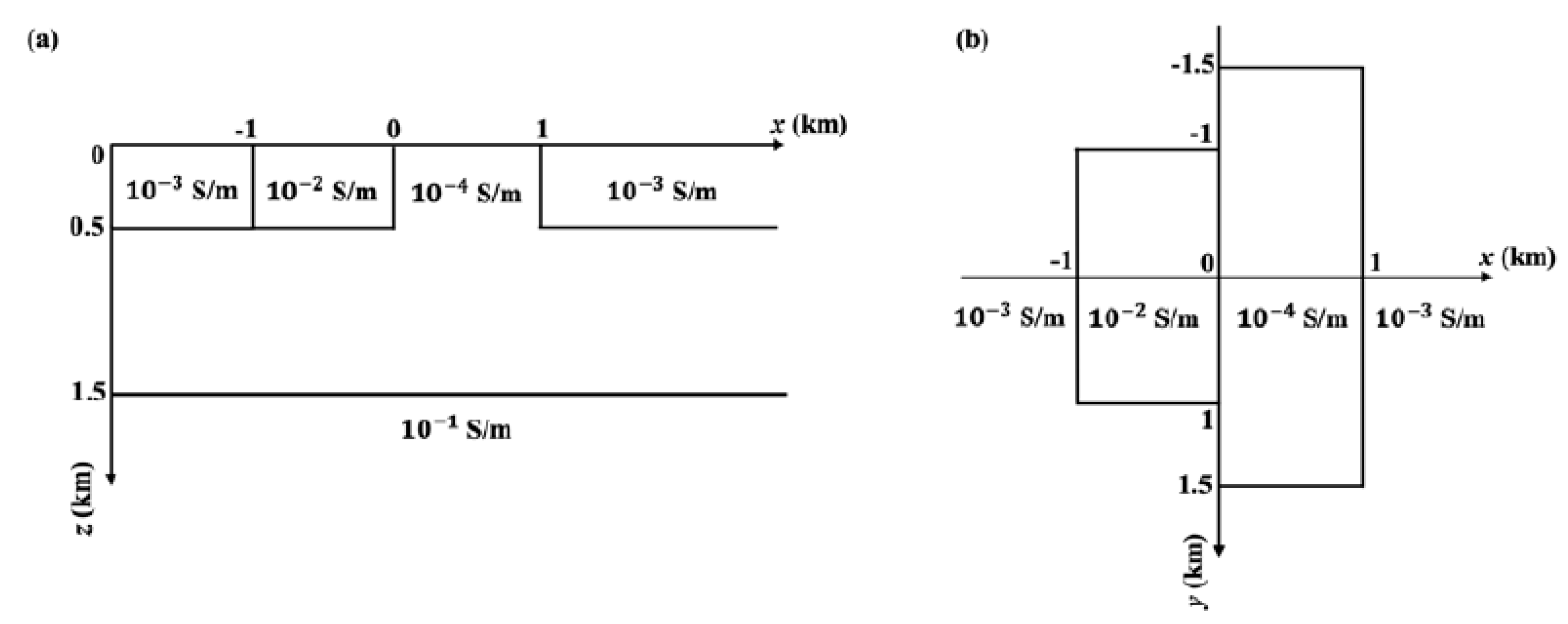
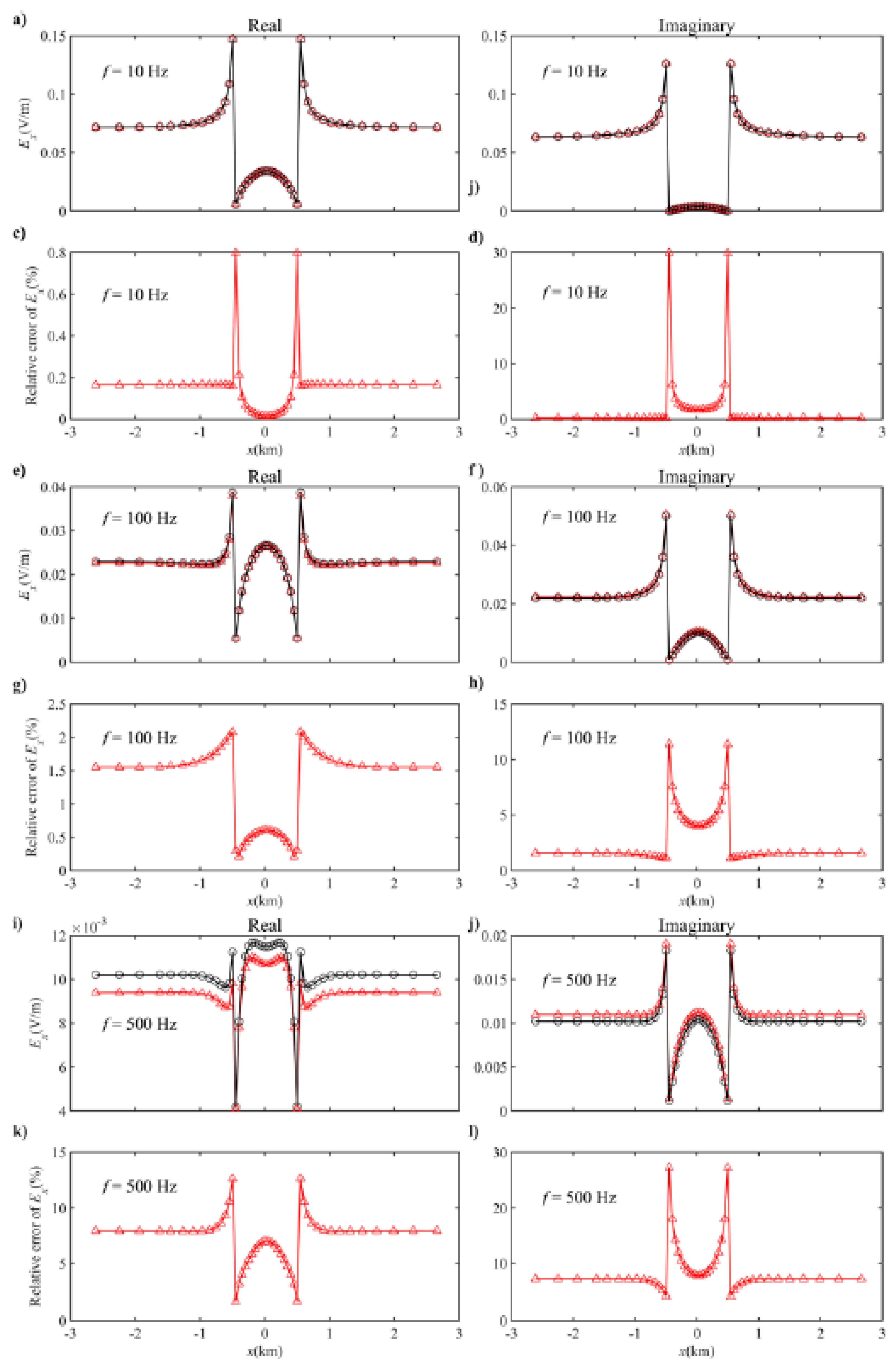
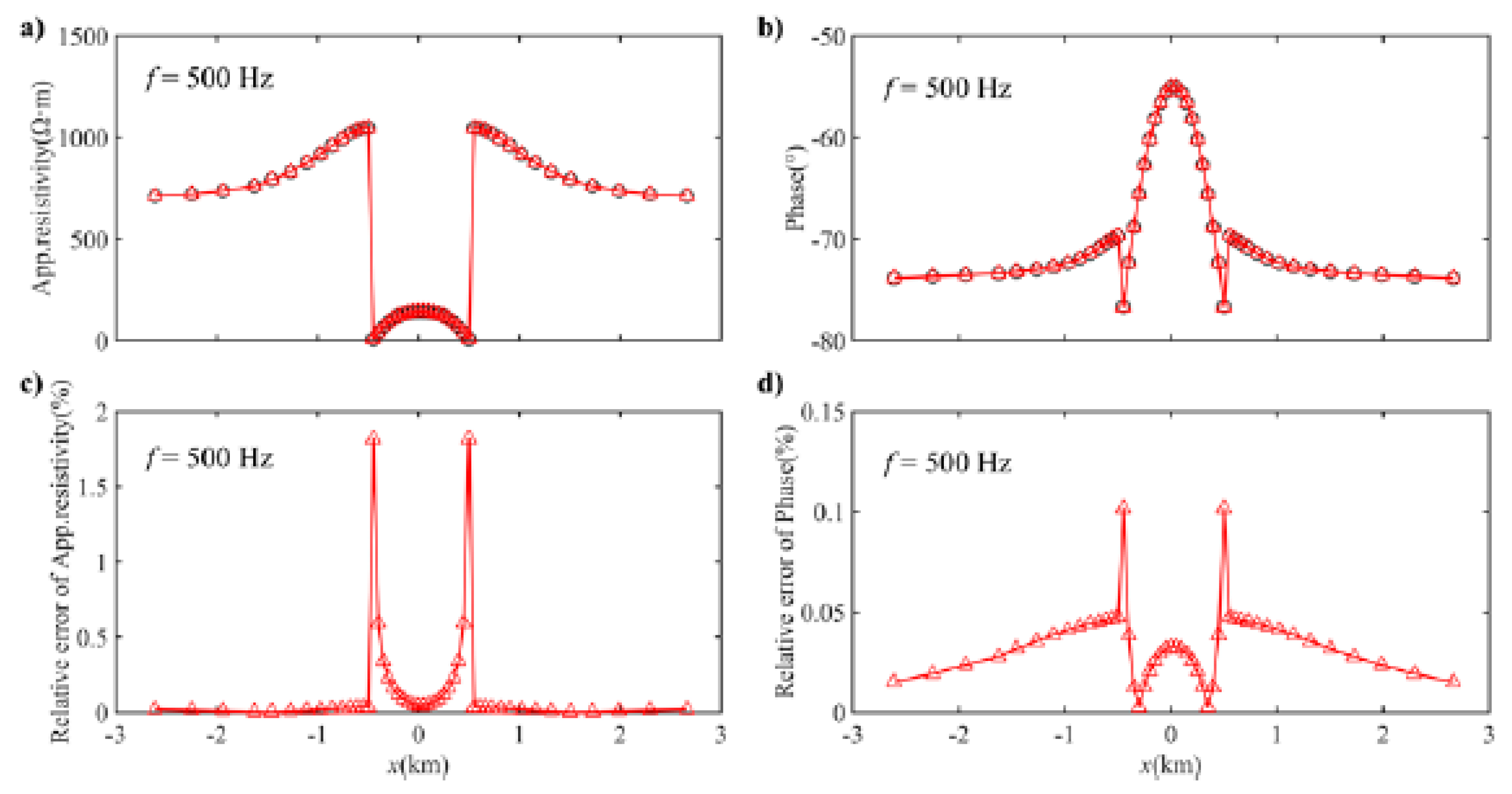
3.3. Models with Topography

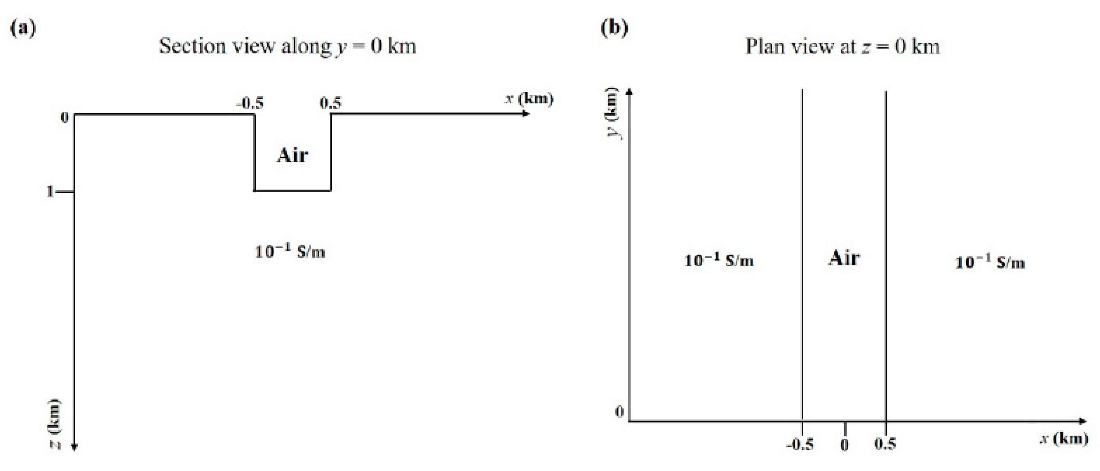
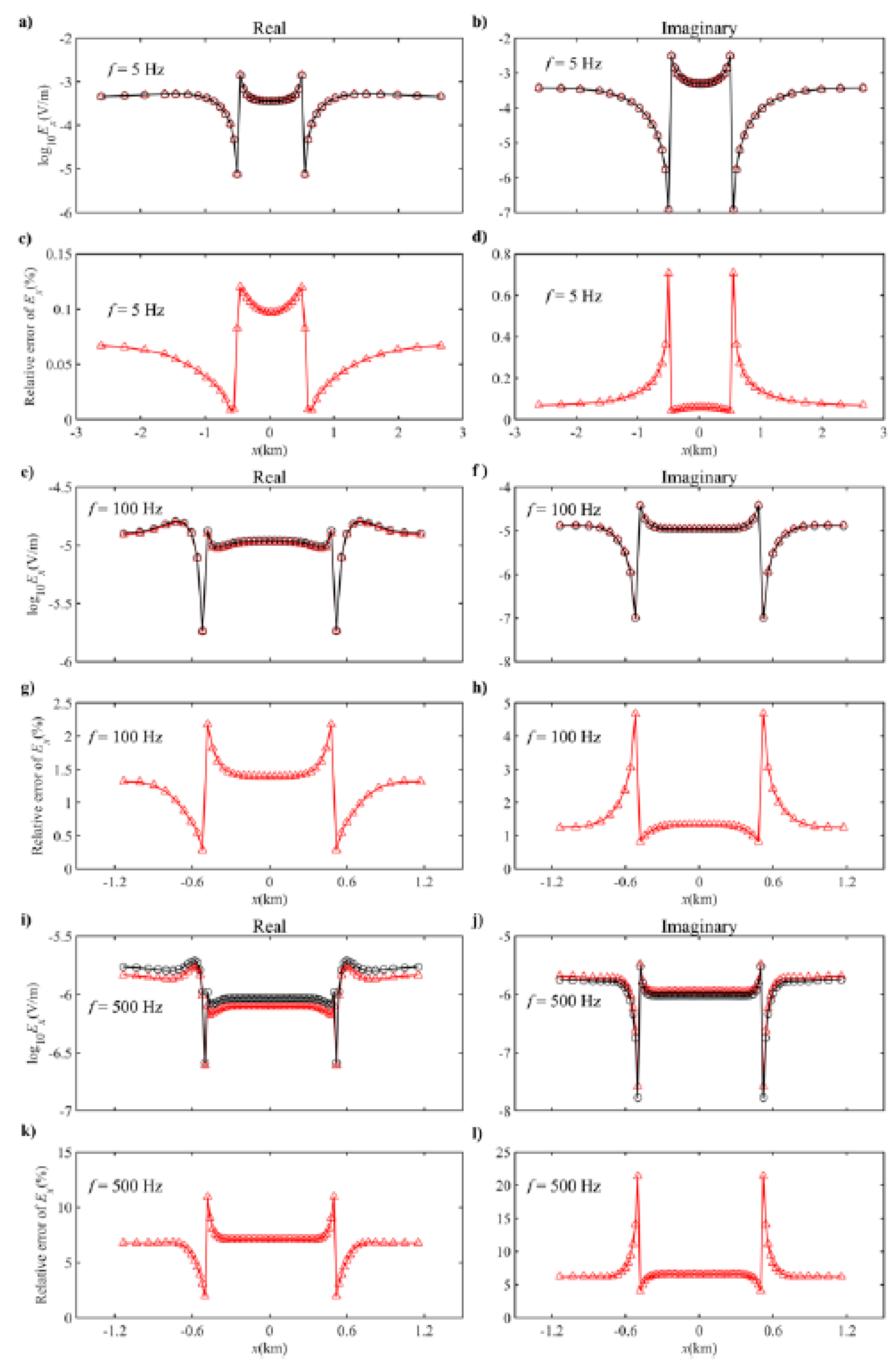
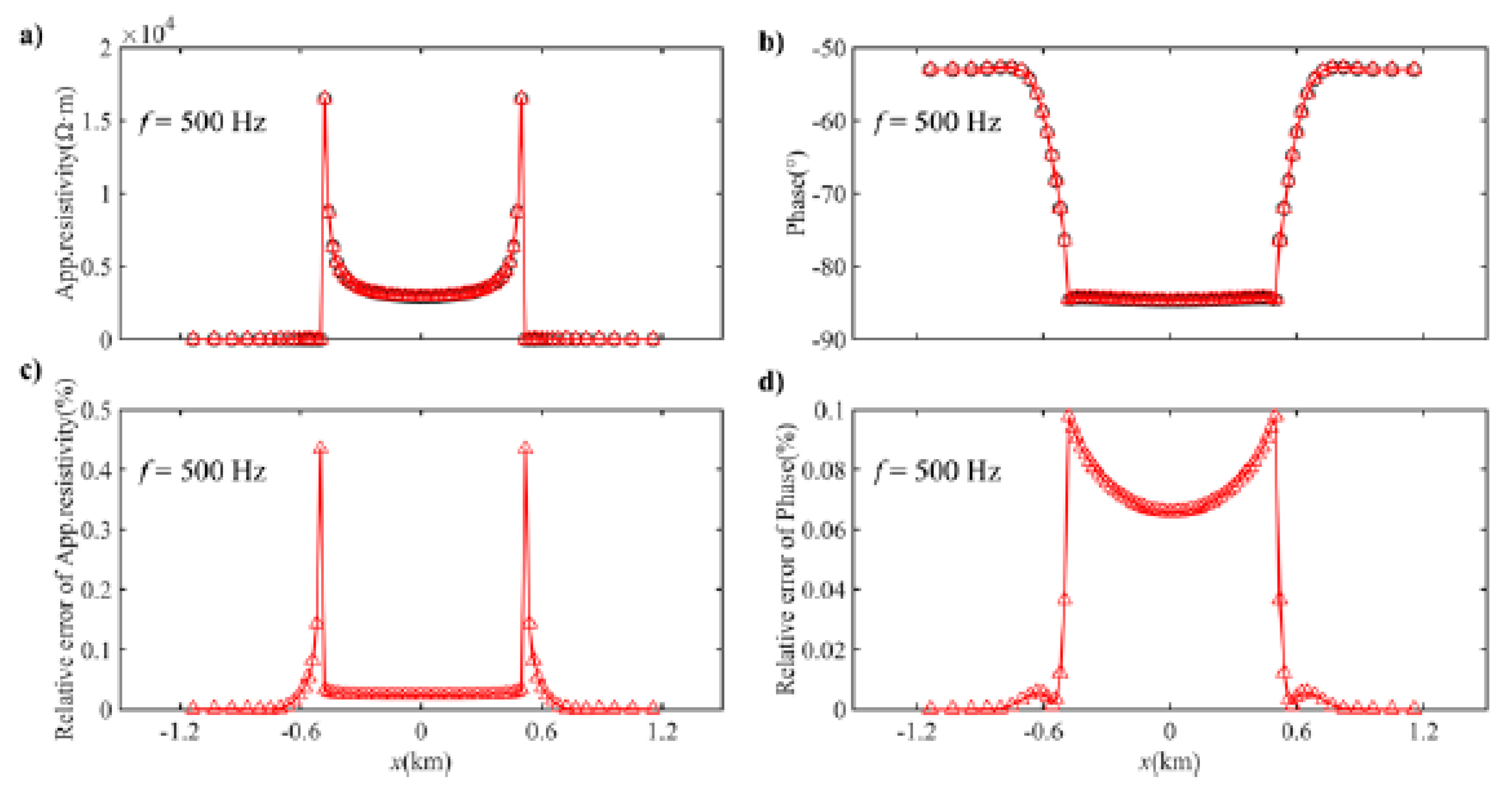
In this section, we design two models with topography (i.e., one canyon model and one steep hill model). The reason to use the rectangular topography models is that finite-difference methods can handle such topography accurately [1]. For cases based on the quasi-static approximation, the conductivity of air layer is set to be 10⁻⁶ S/m. The EM modeling results based on the complete wavenumber are used as the reference solution to calculate the relative errors for those based on the quasi-static approximation. To avoid errors caused by the applied discretization (cell size and used airlayers), different meshes are used for different frequencies (final meshes are examined by comparing their results with those from corresponding finer ones).

3.3.1. Canyon Model

For this model, as shown in Figure 6, the canyon is treated as part of the air layer. The background conductivity is 10⁻¹ S/m. After tests, frequencies considered are 5 × 10⁰, 10², and 5 × 10² Hz. Solutions for cases based on the quasi-static approximation are compared with those using the complete wavenumber along one survey line.

Figure 7 shows the comparison of modeling results at different frequencies for the canyon model by treating the air conductivity differently, along with relative errors for the solution based on the quasi-static approximation. As indicated in the figure, as the frequency increases, the deviation between the two solutions becomes larger, leading to an increase in the relative errors. At a frequency of 5 × 10⁰ Hz, the modeling results from cases in which the air conductivity is treated differently are in good agreement, as indicated in Figure 7 a–d, for both real and imaginary parts of the x-component electrical field, with biggest relative errors of less than 1%. At a frequency of 10² Hz, the comparison is shown in Figure 7 e–h. Most relative errors are larger than 1% for both the real and imaginary parts, with the respective biggest relative errors of 2% and 5%. At 5 × 10² Hz, significant mismatches are shown in Figure 7 i–l for both the real and imaginary parts. The largest relative error reaches 11% for the real part and 21% for the imaginary part. For all frequencies, larger errors are shown for the imaginary part relative to the real part. The comparison for apparent resistivity and phase is shown in Figure 8, indicating that the quasi-static approximation generally works well for apparent resistivity and phase calculations (similar results for other high frequencies).

It is worthy to note that due to the canyon, large relative errors tend to happen at substantially lower frequencies than the corresponding flat model with the quasi-static approximation. This indicates that the existence of the canyon makes the upper limit of frequency, below which the quasi-static approximation is valid, lower than expected. In this case, the quasi-static approximation can affect the EM modeling results significantly at frequencies as low as several hundred Hz.

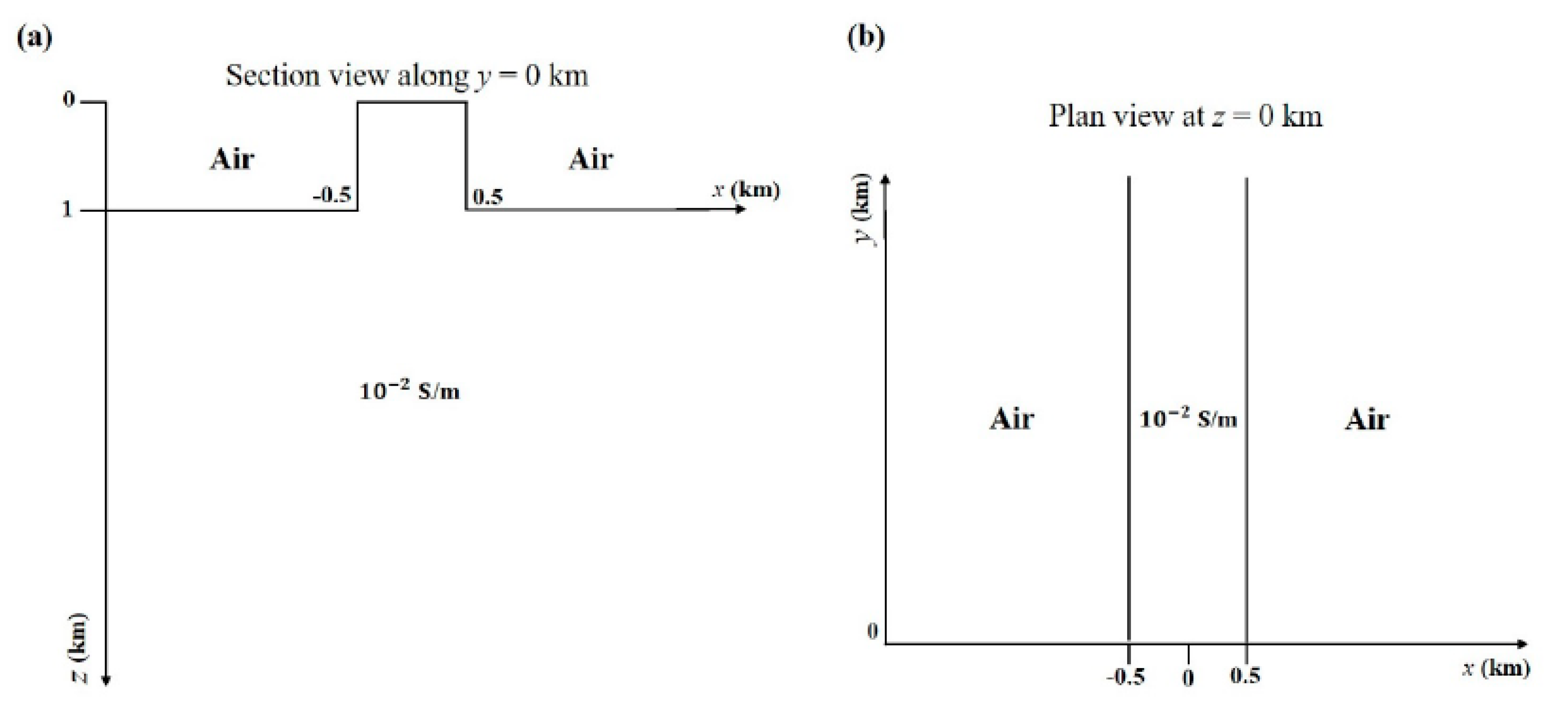
3.3.2. Steep Hill Model

In this part, a steep hill model, as shown in Figure 9, is designed with both height and width of 1 km. The background conductivity is 10⁻² S/m. Frequencies considered are 10¹, 10², and 5 × 10² Hz.

Similarly, solutions for cases based on the quasi-static approximation are compared with those for cases using the complete wavenumber along one survey line.

Figure 10 shows the comparison of modeling results at different frequencies for the steep hill model, along with the relative errors as calculated in Figure 7. Similar to the results indicated in Figure 7, the deviation between the two solutions increases with frequency. At a frequency of 10¹ Hz, the two modeling results are in good agreement, as indicated in Figure 10a–d, for both real and imaginary parts of the x-component electrical field with relative errors much smaller than 1%. As frequency increases to 10² Hz, as shown in Figure 10e–h, the relative errors are mostly larger than 1% for both the real part and the imaginary part (with largest respective relative errors 2% and 11%). At 5 × 10² Hz, as shown in Figure 10i–l, for both the real and imaginary parts, their deviations from the reference solution are substantial. The largest relative error reaches 13% for the real part and 28% for the imaginary part.

Due to the existence of the steep hill, similar to the canyon model case, large relative errors tend to happen at considerably lower frequencies for the quasi-static approximation cases than the corresponding flat model. Similar to the results indicated in the previous case, the steep hill also makes the upper limit of frequency for valid quasi-static approximation, substantially lower than expected (as low as several hundred Hz). This error might be caused by the inaccurate EM description in the air. The comparison of apparent resistivity and phase shown in Figure 11 also indicates that the quasi-static approximation has little effect on the accuracy of apparent resistivity and phase calculations.

4. Conclusions

In this paper, we examine the effect of the quasi-static approximation on the forward modeling of EM diffusion, based on the electric-field formulation. This is carried out by comparing the numerical modeling results from cases using the quasi-static approximation and using the complete wavenumber. For the quasi-static approximation, the conductivity in the air is set to be small values; for cases with the complete wavenumber, zero conductivity is used for the air. Several simple models are designed to verify the numerical solution and study how the assigned conductivity in the air affects the modeling accuracy. One flat model and two models with topography are then designed to examine the effect of the quasi-static approximation on the EM modeling results.

The tests on simple models indicate that our numerical solution with the complete wavenumber is accurate. The quasi-static approximation in the air affects the accuracy of EM simulation based on electric-field formulation. The extent of this impact on the modeling results depends on the conductivity used for the air and the conductivity of the earth, as well as the operating frequency. For a given earth conductivity, a saturation air conductivity (a further decrease in conductivity cannot further improve the modeling accuracy) exists. A decrease in the conductivity of the earth can result in a lower upper frequency boundary above which large errors will occur and the quasi-static approximation is violated. While the flat complex model exhibits similar behavior as the two simple models, two models with uneven surface act in a different way. For the two models with undulating surfaces, the accuracy of the numerical results for EM fields deteriorates substantially at much lower frequencies (as low as several hundred Hz), most likely due to the violation of the quasi-static approximation in the air. However, the apparent resistivity and phase results are generally accurate at the quasi-static approximation at frequencies considered in this paper. For EM explorations in uneven topographical areas based on the interpretation of EM fields, the quasi-static approximation is likely to be problematic at frequencies as low as several hundred Hz. In such applications, the use of the complete wavenumber may be required.

References

1. Ward, S.H.; Hohmann, G.W. Electromagnetic theory for geophysical applications. In Electromagnetic Methods in Applied Geophysics: Volume 1, Theory; Society of Exploration Geophysicists: Tulsa, Oklahoma, 1988; pp. 130–311. [Google Scholar]
2. Zhdanov, M.S.; Lee, S.K.; Yoshioka, K. Integral equation method for 3D modeling of electromagnetic fields in complex structures with inhomogeneous background conductivity. Geophysics 2006, 71, 333–345. [Google Scholar] [CrossRef]
3. Vozoff, K. Electromagnetic methods in applied geophysics. Geophys. Surv. 1980, 4, 9–29. [Google Scholar] [CrossRef]
4. Avdeev, D.B. Three-dimensional electromagnetic modelling and inversion from theory to application. Surv. Geophys. 2005, 26, 767–799. [Google Scholar] [CrossRef]
5. Farquharson, C.G.; Craven, J.A. Three-dimensional inversion of magnetotelluric data for mineral exploration: An example from the McArthur River uranium deposit, Saskatchewan, Canada. J. Appl. Geophys. 2009, 68, 450–458. [Google Scholar] [CrossRef]
6. Zhang, K.; Wei, W.; Lu, Q.; Dong, H.; Li, Y. Theoretical assessment of 3-D magnetotelluric method for oil and gas exploration: Synthetic examples. J. Appl. Geophys. 2014, 106, 23–36. [Google Scholar] [CrossRef]
7. Beka, T.I.; Smirnov, M.; Birkelund, Y.; Senger, K.; Bergh, S.G. Analysis and 3D inversion of magnetotelluric crooked profile data from central Svalbard for geothermal application. Tectonophysics 2016, 686, 98–115. [Google Scholar] [CrossRef]
8. Newman, G.A.; Alumbaugh, D.L. Three-dimensional magnetotelluric inversion using non-linear conjugate gradients. Geophys. J. Int. 2000, 140, 410–424. [Google Scholar] [CrossRef] [Green Version]
9. Xiang, E.; Guo, R.; Dosso, S.E.; Liu, J.; Dong, H.; Ren, Z. Efficient hierarchical trans-dimensional Bayesian inversion of magnetotelluric data. Geophys. J. Int. 2018, 213, 1751–1767. [Google Scholar] [CrossRef]
10. Miensopust, M.P.; Queralt, P.; Jones, A.G.; The 3D MT Modellers. Magnetotelluric 3-D inversion—A review of two successful workshops on forward and inversion code testing and comparison. Geophys. J. Int. 2013, 193, 1216–1238. [Google Scholar] [CrossRef] [Green Version]
11. Ren, Z.; Kalscheuer, T.; Greenhalgh, S.; Maurer, H. A goal-oriented adaptive finite-element approach for plane wave 3-D electromagnetic modelling. Geophys. J. Int. 2013, 194, 700–718. [Google Scholar] [CrossRef] [Green Version]
12. Wang, Y.; Liu, J.; Liu, R.; Guo, R.; Feng, D. Frequency-domain magnetotelluric footprint analysis for 3D earths. J. Geophys. Eng. 2019, 16, 1151–1163. [Google Scholar] [CrossRef] [Green Version]
13. Wannamaker, P.E. Advances in three-dimensional magnetotelluric modeling using integral equations. Geophysics 1991, 56, 1716–1728. [Google Scholar] [CrossRef]
14. Avdeev, D.; Knizhnik, S. 3D integral equation modeling with a linear dependence on dimensions. Geophysics 2009, 74, 89–94. [Google Scholar] [CrossRef]
15. Newman, G.A.; Alumbaugh, D.L. Three-dimensional induction logging problems, Part 2: A finite-difference solution. Geophysics 2002, 67, 484–491. [Google Scholar] [CrossRef]
16. Farquharson, C.G.; Miensopust, M.P. Three-dimensional finite-element modelling of magnetotelluric data with a divergence correction. J. Appl. Geophys. 2011, 75, 699–710. [Google Scholar] [CrossRef]
17. da Silva, N.V.; Morgan, J.V.; MacGregor, L.; Warner, M. A finite element multifrontal method for 3D CSEM modeling in the frequency domain. Geophysics 2012, 77, 101–115. [Google Scholar] [CrossRef]
18. Ansari, S.; Farquharson, C.G. 3D finite-element forward modeling of electromagnetic data using vector and scalar potentials and unstructured grids. Geophysics 2014, 79, 149–165. [Google Scholar] [CrossRef]
19. Liu, J.; Liu, P.; Tong, X. Three-dimensional Land FD-CSEM Regularized Inversion Based on Edge Finite-element Method. J. Environ. Eng. Geophys. 2018, 23, 211–222. [Google Scholar]
20. Liu, R.; Guo, R.; Liu, J.; Liu, Z. An Efficient Footprint-Guided Compact Finite Element Algorithm for 3-D Airborne Electromagnetic Modeling. IEEE Geosci. Remote Sens. Lett. 2019, 16, 1809–1813. [Google Scholar] [CrossRef]
21. Mackie, R.L.; Smith, J.T.; Madden, T.R. Three-dimensional electromagnetic modeling using finite difference equations: The magnetotelluric example. Radio Sci. 1994, 29, 923–935. [Google Scholar] [CrossRef]
22. Siripunvaraporn, W.; Egbert, G.; Lenbury, Y. Numerical accuracy of magnetotelluric modeling: A comparison of finite difference approximations. Earth Planets Space 2002, 54, 721–725. [Google Scholar] [CrossRef] [Green Version]
23. Streich, R. 3D finite-difference frequency-domain modeling of controlled-source electromagnetic data: Direct solution and optimization for high accuracy. Geophysics 2009, 74, 95–105. [Google Scholar] [CrossRef]
24. Kelbert, A.; Meqbel, N.; Egbert, G.D.; Tandon, K. ModEM: A modular system for inversion of electromagnetic geophysical data. Comput. Geosci. 2014, 66, 40–53. [Google Scholar] [CrossRef]
25. Li, J.; Liu, J.; Egbert, G.D.; Liu, R.; Guo, R.; Pan, K. An efficient preconditioner for 3-D finite difference modeling of the electromagnetic diffusion process in the frequency domain. IEEE Trans. Geosci. Remote Sensi. 2019, 58, 500–509. [Google Scholar] [CrossRef]
26. Varilsuha, D.; Candansayar, M.E. 3D magnetotelluric modeling by using finite-difference method: Comparison study of different forward modeling approaches. Geophysics 2018, 83, 51–60. [Google Scholar] [CrossRef]
27. Um, E.S.; Harris, J.M.; Alumbaugh, D.L. An iterative finite element time-domain method for simulating three-dimensional electromagnetic diffusion in earth. Geophys. J. Int. 2012, 190, 871–886. [Google Scholar] [CrossRef] [Green Version]
28. Cai, H.; Hu, X.; Li, J.; Endo, M.; Xiong, B. Parallelized 3D CSEM modeling using edge-based finite element with total field formulation and unstructured mesh. Comput. Geosci. 2017, 99, 125–134. [Google Scholar] [CrossRef]
29. Liu, R.; Guo, R.; Liu, J.; Ma, C.; Guo, Z. A hybrid solver based on the integral equation method and vector finite-element method for 3D controlled-source electromagnetic method modeling. Geophysics 2018, 83, 319–333. [Google Scholar] [CrossRef]
30. Egbert, G.D.; Kelbert, A. Computational recipes for electromagnetic inverse problems. Geophys. J. Int. 2012, 189, 251–267. [Google Scholar] [CrossRef] [Green Version]
Figure 1. Definition of the electric and magnetic field components on the staggered grid.
Applsci 10 02744 g001
Figure 2. Comparison of the E x solutions from cases based on the quasi-static approximation with 10−4 (orange dashed lines), 10−6 (purple asterisk lines), 10−8 (dark green square lines), and 10−10 S/m (red circle lines) for air conductivity, and the one with the complete wavenumber (blue dotted cross lines) along with the analytical solution (solid lines) for model I. (a) the real part and (b) the imaginary part of E x are indicated, and the relative errors of (c) the real partand (d) the imaginary part of E x are indicated.
Applsci 10 02744 g002
Figure 3. Comparison of the E x solutions from cases based on the quasi-static approximation with 10−4 (orange dashed lines), 10−6 (purple asterisk lines), 10−8 (dark green square lines), and 10−10 S/m (red circle lines) for air conductivity, and the one with the complete wavenumber (blue dotted cross lines) along with the analytical solution (solid lines) for model II. (a) the real part and (b)the imaginary part of E x are indicated and the relative errors of (c) the real part of and (d) the imaginary part of E x are indicated.
Applsci 10 02744 g003
Figure 4. COMMEMI 3D-2 test model: (a) x-z section view along y = 0, (b) x-y plan view at z = 0.
Applsci 10 02744 g004
Figure 5. Comparison of the E x numerical solutions from the case based on the quasi-static approximation (upward-pointing triangle lines) with 10−8 S/m for air conductivity, and the one with the complete wavenumber (circle lines) at frequencies of (ad) 103, (eh) 2×10³, and (il) 5×10³ Hz for the 3D flat model. The relative errors are referenced to the results based on the use of the complete wavenumber.
Applsci 10 02744 g005
Figure 6. Sketch of the canyon model. (a) x-z section view along y = 0 km, (b) x-y plan view at z = 0 km.
Applsci 10 02744 g006
Figure 7. Comparison of the E x numerical solutions from the case based on the quasi-static approximation (upward-pointing triangle lines)) with 10−6 S/m for air conductivity, and the one with the complete wavenumber (circle lines) at frequencies of (ad) 5 × 100, (eh) 102, and (il) 5 × 10² Hz for the canyon model. The relative errors are referenced to the results based on the use of the complete wavenumber.
Applsci 10 02744 g007
Figure 8. Comparison plots of the apparent resistivity (a,c) and phase (b,d) from the case based on the quasi-static approximation (upward-pointing triangle lines)) with 10−6 S/m for air conductivity, and the one with the complete wavenumber (circle lines) at a frequency of 5 × 10² Hz for the canyon model. The relative errors are referenced to the results based on the use of the complete wavenumber.
Applsci 10 02744 g008
Figure 9. Sketch of the steep hill model. (a) x-z section view along y = 0, (b) x-y plan view at z = 0.
Applsci 10 02744 g009
Figure 10. Comparison of the E x numerical solutions from the case based on the quasi-static approximation (upward-pointing triangle lines) with 10−6 S/m for air conductivity, and the one with the complete wavenumber (circle lines) at frequencies of (ad) 101, (eh) 102, and (il) 5 × 10² Hz for the steep hill model. The relative errors are referenced to the results based on the use of the complete wavenumber.
Applsci 10 02744 g010
Figure 11. Comparison plots of the apparent resistivity (a,c) and phase (b,d) from the case based on the quasi-static approximation (upward-pointing triangle lines)) with 10−6 S/m for air conductivity, and the one with the complete wavenumber (circle lines) at frequency of 5 × 10² Hz for the steep hill model. The relative errors are referenced to the results based on the use of the complete wavenumber.
Applsci 10 02744 g011