Evaluating the Impact of Turbulence Closure Models on Solute Transport Simulations in Meandering Open Channels

Abstract

River meanders form complex 3D flow patterns, including secondary flows and flow separation. In particular, the flow separation traps solutes and delays their transport via storage effects associated with recirculating flows. The simulation of the separated flows highly relies in the performance of turbulence models. Thus, these closure schemes can control dispersion behaviors simulated in rivers. This study performs 3D simulations to quantify the impact of the turbulence models on solute transport simulations in channels under different sinuosity conditions. The 3D Reynolds-averaged Navier-Stokes equations coupled with the $k-\epsilon$, $k-\omega$ and SST $k-\omega$ models are adopted for flow simulations. The 3D Lagrangian particle-tracking model simulates solute transport. An increase in sinuosity causes strong transverse gradients of mean velocity, thereby driving the onset of the separated flow recirculation along the outer bank. Here, the onset and extent of the flow separation are strongly influenced by the turbulence models. The $k-\epsilon$ model fails to reproduce the flow separation or underestimates its size. As a result, the $k-\epsilon$ model yields residence times shorter than those of other models. In contrast, the SST $k-\omega$ model exhibits a strong tailing of breakthrough curves by generating more pronounced flow separation.

1. Introduction

River topography exerts a first-order control on flow and solute transport mechanisms. Especially in river bends, complex three-dimensional (3D) flow structures such as secondary flows and recirculating flows develop due to the local imbalance between the centrifugal force and the pressure force [1,2]. The velocity gradient driven by the secondary flow increases the longitudinal dispersion via shear flow effects [3]. The helical motion of the secondary flow not only impacts the primary flow but also stimulates the transverse mixing [4,5]. Moreover, the dead zones with vigorous recirculating flows, developed by the channel irregularity, trap a solute cloud and induce the non-Fickian dispersion characterized as an elevated concentration of tracers downstream at late times [6,7]. Hence, the aforementioned flow features are required to be described adequately with numerical models for accurate prediction of solute dispersion behaviors in surface water systems.

There have been numerous studies that use the 3D Reynolds-averaged Navier-Stokes (RANS) model for reproducing flow fields in large-scale meandering channels, honoring the reasonable computational cost compared to large eddy simulations (LES) and direct numerical simulations (DNS) [8,9,10,11]. The main advantage of the LES model is that the near-bank secondary flow within the channel bend is superiorly reproduced compared to the RANS model [12,13]. The previous experimental studies; however, reported that the near-bank cell shrinks as the Froude number increases [14] and possesses relatively weaker strength and smaller size than those of the main secondary flow cell at the central regions [15]. Therefore, in consideration of computational efficiency, the RANS model is an acceptable alternative for computing large-scale flow structures and shear flow dispersion accordingly in meandering channels.

The flow structures simulated with the 3D RANS model substantially rely on turbulence models. Among several turbulence models, two-equation models are widely used for flow analysis. Since the research of Demuren and Rodi [16], the $k-\epsilon$ model has widely been employed for hydrodynamic simulations in meander bends due to the computational stability with good convergence, adequately capturing entire flow patterns of the secondary circulations [17,18,19,20]. However, the $k-\epsilon$ model often fails to reproduce the adverse pressure gradient flows, thus causing inaccurate results in boundary layer flows [21]. The $k-\omega$ model overcomes the disadvantages of the $k-\epsilon$ model by achieving more precise simulations in the wall boundary layers under the adverse pressure gradient conditions [22]. Yet, both the $k-\epsilon$ and $k-\omega$ models lack the ability to reproduce massively separated flows under severe adverse pressure gradients [23,24]. As an alternative to these turbulence models, Menter [25] proposed the shear stress transport (SST) $k-\omega$ model, which combines the robust formulations of the $k-\omega$ model for the near-wall regions and the $k-\epsilon$ model for the free-flow regions. The SST $k-\omega$ model has been shown to accurately predict the onset and extent of the flow separation in complex geometric configurations [26,27,28].

In rivers and streams, the flow separation is frequently observed owing to the intricate flow patterns associated with geomorphic features of rivers, such as confluence, pool-riffle sequence, bifurcation, and meander [29,30]. Notably, the experimental studies of Blanckaert [31,32,33] revealed that sharp channel curvature forms a pronounced flow separation near the bend apex because of significant adverse pressure gradients, and this curvature-induced flow separation manifests as a recirculation zone in the horizontal plane. The lateral recirculation zone (dead zone) acts as a surface storage zone, which induces anomalously long residence times of solutes via trapping effects, then drive the non-Fickian tailing behaviors [34,35]. Thus, it is critical to accurately predict the onset and size of the flow separation in meander bends for successfully capturing the non-Fickian transport signatures in riverine environments. As aforementioned, the prediction of the flow separation is highly sensitive to turbulence models. The $k-\epsilon$ model has popularly been adopted for simulations of solute mixing in curved channels [16,36,37], whereas the impact of turbulence models on solute transport is rarely assessed. Furthermore, the non-Fickian mixing properties associated with the horizontal flow recirculation within the meander bend have not been deeply discussed with resepct to turbulence models and channel sinuosity.

The present work sheds light on the impact of turbulence closure models on solute transport and the non-Fickian mixing behaviors in meandering channels having different sinuosity levels. First, 3D flow characteristics in meandering open channels are reproduced using the 3D RANS model incorporated with a variety of turbulence closure schemes including the $k-\epsilon$, $k-\omega$ and SST $k-\omega$ models. The flow simulation results are compared by changing meander geometry to scrutinize the influence of the turbulence models on the secondary flow and flow separation structures in channels across a diverse range of sinuosity. With the 3D flow fields obtained from the three different turbulence models, the solute transport is then simulated adopting the 3D Lagrangian particle-tracking (LPT) algorithm. This study eventually aims to unravel how the turbulence models influence the solute transport simulations in meandering open-channel flows taking into account their performance in reproducing the meander-driven flow features, especially the separated flow recirculation.

2. Methodology

2.1. Hydrodynamic Model

This study resolves 3D flow structures in meandering channels using the 3D RANS equations, which are solved with OpenFOAM, an open-source computational fluid dynamics library based on the finite volume method. The OpenFOAM-based RANS models have been extensively used for analysis of open channel flows including bed erosion [28,38], hydraulic jump [39,40,41], spillway jet [41], flows around hydraulic structures [42,43,44], and coupled flows with porous media [45]. For incompressible fluid flows, the 3D RANS model adopts the Reynold approximation of continuity and momentum equations as follows:

$$\frac{\partial U_i}{\partial x_i}=0$$

(1)

$$\frac{\partial U_i}{\partial t}+U_j\frac{\partial U_i}{\partial x_j}=-\frac{1}{\rho }\frac{\partial P}{\partial x_i}+\frac{\partial }{\partial x_j}\left[\nu \left(\frac{\partial U_i}{\partial x_j}+\frac{\partial U_j}{\partial x_i}\right)\right]-\frac{\partial }{\partial x_j}\overline{u_i{u}_j}$$

(2)

where $U_i$ is the time-averaged velocity in the Cartesian coordinate; $P$ is the pressure; $\rho$ is the fluid density; $\nu$ is the kinematic viscosity; $u_i$ is the velocity fluctuation; and $\overline{u_i{u}_j}$ is the Reynolds stress. Under the Boussinesq approximation, $\overline{u_i{u}_j}$ is defined as:

$$-\overline{u_i{u}_j}={\nu }_t\left(\frac{\partial U_i}{\partial x_j}+\frac{\partial U_j}{\partial x_i}\right)+\frac{2}{3}k{\delta }_{ij}$$

(3)

where ${\nu }_t$ is the turbulent eddy viscosity; $k$ is the turbulent kinetic energy; ${\delta }_{ij}$ is the Kronecker delta. To close Equation (2) by resolving ${\nu }_t$, this study employs two-equation turbulence closure models such as $k-\epsilon$, $k-\omega$ and SST $k-\omega$ models available with the Open FOAM library.

In the $k-\epsilon$ model, ${\nu }_t$ is modeled with the turbulent kinetic energy, $k$ and the turbulent energy dissipation, $\epsilon$ using the relation described as:

$${\nu }_t=\rho C_{\mu }\frac{k^2}{\epsilon }$$

(4)

where $C_{\mu }$ is the empirical constant. The additional transport equations for simulating $k$ and $\epsilon$ are given as:

$$\frac{\partial k}{\partial t}+\frac{\partial \left(U_{i}k\right)}{\partial x_i}=\frac{\partial }{\partial x_j}\left[\left(\frac{{\nu }_t}{{\sigma }_k}+\nu \right)\frac{\partial k}{\partial x_j}\right]-\epsilon +G_k$$

(5)

$$\frac{\partial \epsilon }{\partial t}+\frac{\partial \left(U_i\epsilon \right)}{\partial x_i}=\frac{\partial }{\partial x_j}\left[\left(\frac{{\nu }_t}{{\sigma }_{\epsilon }}+\nu \right)\frac{\partial \epsilon }{\partial x_j}\right]+C_{\epsilon 1}{G}_k\frac{\epsilon }{k}-C_{\epsilon 2}\frac{{\epsilon }^2}{k}$$

(6)

where ${\sigma }_k$, ${\sigma }_{\epsilon }$, $C_{\epsilon 1}$, and $C_{\epsilon 2}$ are the empirical constants; and $G_k$ is the production of turbulent kinetic energy due to the mean velocity gradient. The empirical constants of the $k-\epsilon$ model have been reported as $C_{\mu }=0.09$, $C_{\epsilon 1}=1.44$, $C_{\epsilon 2}=1.92$, ${\sigma }_k=1.0$, ${\sigma }_{\epsilon }=1.3$ at high Reynolds number [46]. The $k-\epsilon$ model is well known as the simplest turbulence model providing acceptable accuracy for diverse hydraulic problems with good convergence. However, the inherent limitations originated from the turbulent viscosity relation in Equation (4) and the $\epsilon$ equation lead to inaccurate simulations for flows near the boundary layers. Therefore, the damping function is required to correct the overestimated ${\nu }_t$ within the boundary flow [47].

The $k-\omega$ model uses the specific dissipation rate, $\omega =\epsilon /k$ instead of $\epsilon$ to model ${\nu }_t$ defined as:

$${\nu }_t=\frac{k}{\omega }$$

(7)

To resolve Equation (7), the additional transport equations for $k$ and $\omega$ are presented as:

$$\frac{\partial k}{\partial t}+\frac{\partial \left(U_{i}k\right)}{\partial x_i}=\frac{\partial }{\partial x_j}\left[\left(\frac{{\nu }_t}{{\sigma }_k}+\nu \right)\frac{\partial k}{\partial x_j}\right]+G_k-{\beta }^{\ast }k\omega$$

(8)

$$\frac{\partial \omega }{\partial t}+\frac{\partial \left(U_i\omega \right)}{\partial x_i}=\frac{\partial }{\partial x_j}\left[\left(\frac{{\nu }_t}{{\sigma }_{\omega }}+\nu \right)\frac{\partial \omega }{\partial x_j}\right]+\alpha G_{\omega }\frac{\omega }{k}-\beta {\omega }^2$$

(9)

where ${\sigma }_{\omega }$, $\alpha$, $\beta$, and ${\beta }^{\ast }$ are the empirical constants; and $G_{\omega }$ is the production of the dissipation rate. Here, the empirical constants are suggested as ${\sigma }_k=2$, ${\sigma }_{\omega }=2$, $\alpha =0.55$, $\beta =0.075$, and ${\beta }^{\ast }=0.09$ [22]. The $k-\omega$ model is superior to the $k-\epsilon$ model for simulating the boundary layer flows and streamwise pressure gradients. Nevertheless, the $k-\omega$ model has a disadvantage in that the simulation results are sensitive to the free-stream boundary conditions [25].

The SST $k-\omega$ model compensates for the shortcomings of these two turbulence models by implementing the $k-\omega$ model in the boundary layers and the $k-\epsilon$ model in the free-shear layers. Thus, the SST $k-\omega$ model is advantageous to reproduce the wall-bounded flows under low Reynolds conditions without extra damping functions. In the SST $k-\omega$ model, ${\nu }_t$ is modeled as:

$${\nu }_t=\frac{a_{1}k}{\max \left(a_1\omega ,S{F}_2\right)}$$

(10)

where $a_1$ is the closure coefficient; $S$ is the absolute value of the vorticity; and $F_2$ is the blending function that gives unity for the boundary layers and zero for the free-shear layers. The SST $k-\omega$ model adopts the reformulated $\omega$ equation as follows:

$$\frac{\partial \omega }{\partial t}+\frac{\partial \left(U_i\omega \right)}{\partial x_i}=\frac{\partial }{\partial x_j}\left[\left(\frac{{\nu }_t}{{\sigma }_{\omega }}+\nu \right)\frac{\partial \omega }{\partial x_j}\right]+\alpha S^2-\beta {\omega }^2+2\left(1-F_1\right)\frac{{\sigma }_{w2}}{\omega }\frac{\partial k}{\partial x_i}\frac{\partial \omega }{\partial x_i}$$

(11)

where $F_2$ is the auxiliary relation; and ${\sigma }_{\omega 2}$ is an empirical constant. The SST $k-\omega$ model exhibits improved simulation results for adverse pressure gradient flows, thereby accurately reproducing the pressure-induced flow separation [21]. Zeng et al. [48] simulated flow and sediment transport in curved channels using the SST $k-\omega$ model, and this turbulence model was found to adequately predict changes in bed elevation by well reproducing 3D flow features in the channel bends. Moreover, Kang et al. [49] successfully applied the SST $k-\omega$ model to capture flow characteristics of a natural-like meandering stream located in the St. Anthony Falls Laboratory Outdoor StreamLab, University of Minnesota. They compared simulation results of the $k-\omega$ and SST $k-\omega$ models with LES and field observation data. As a result, the SST $k-\omega$ model shows close agreement with the validation data sets, while the $k-\omega$ model overestimates turbulent kinetic energy. Furthermore, Kang and Sotiropoulos [50] demonstrated that the SST $k-\omega$ model accurately simulates 3D free flows past hydraulic structures and over complex topography of a meandering channel.

2.2. Solute Tansport Model

The transport of solute particles is simulated with the 3D LPT model. In general, the complex interplay between advection, molecular diffusion, and turbulent diffusion governs the solute transport. In turbulent open-channel flow systems, the molecular diffusion can be neglected because, in terms of length scale, the turbulent diffusion is usually dominant over the molecular diffusion. Hence, the solute particle motion is governed by 3D Langevin equations defined as:

$$x_i(t+\Delta t)=x_i(t)+\left[U_i(x_i)+u_i(x_i,t)\right]\Delta t$$

(12)

where $x_i(t)$ is the particle position at $t$; $U_i(x_i)$ is the mean velocity determining the advection process, as a function of space; and $u_i(x_i,t)$ is the instantaneous velocity fluctuation, which governs the turbulent diffusion process and varies spatiotemporally, depending on time and length scale of turbulent eddies.

Since the RANS models are not capable of reproducing the fluctuating velocity, it is necessary to model $u_i(x_i,t)$ in order to consider the turbulent diffusion effects on particle dispersion. This study models the particle dispersion via the discrete random walk (DRW) method suggested by Gosman and Loannides [51]. This stochastic particle dispersion model characterizes the turbulent diffusion process using the RANS-simulated turbulence variables of $k$, $\epsilon$, and $\omega$, and it has successfully been applied to simulate sediment and solute dispersion in turbulent open-channel flows [44,51]. In particular, Shams et al. [52] adequately simulated the effects of the secondary flow on sediment transport and deposition in a meandering channel using the DRW model. However, the role of the meander-driven flow separation was not investigated in this study due to the channel topography with mildly curved bends. The DRW model calculates $u_i(x_i,t)$ from $k$ using the relation below:

$$u_i(x_i,t)=\zeta \sqrt{2k/3}$$

(13)

where $\zeta$ is the normally distributed random number with a zero mean and a unit variance, which represent the arbitrary motion of the turbulent eddy. Here, $\zeta$ is renewed after each lifetime (time scale) of the turbulent eddy, which is calculated as $k/\epsilon$ or $1/\omega$. Therefore, the DRW model can consider both length scale and time scale of the turbulent eddy on particle dispersion using the RANS simulation results without instantaneous velocity fields only available with computationally intensive LES and DNS. References for detailed implementation of the DRW method are provided in Gosman and Loannides [51] and related application studies [53,54].

2.3. Geometric Setups

Hey [55] surveyed geomorphic characteristics of meandering rivers and retrieved the empirical relations between geometric parameters of the river geometries from the field observation, described as follows:

$$R_c=(360/\theta )W$$

(14)

$$\lambda =4\sin (\theta /2)R_c=(1,440/\theta )\sin \left(\theta /2\right)W$$

(15)

where $R_c$ is the radius of curvature; $\theta$ is the arc angle; $W$ is the channel width; and $\lambda$ is the wavelength. These geometric parameters representing the meander shape are illustrated in Figure 1.

Based on Hey’s relations, this study generates meandering channels having three different channel curvatures, as shown in Figure 1. Here, a variation of $\theta$ between 180 and 210° produces sinuosity ranging from 1.36 to 1.90, as summarized in

Table 1. Geometric parameters of meandering channels.

Case	${\mathit{L}}_{\mathit{s}}\left(\mathbf{m}\right)$	$\mathit{\theta }$ (°)	$\mathit{\lambda }$ (m)	${\mathit{R}}_{\mathit{c}}\left(\mathbf{m}\right)$	${\mathit{R}}_{\mathit{c}}/\mathit{W}$	$\mathit{L}/{\mathit{L}}_{\mathit{s}}$
S136	150	150	21.70	5.62	2.40	1.36
S157	131	180	18.72	4.68	2.00	1.57
S190	108	210	15.50	4.00	1.71	1.90

. Please note that sinuosity is defined as $L/L_s$, where $L$ and $L_s$ indicate the channel (curvilinear) length and linear distance between the inlet and outlet, respectively. The generated channels consist of 12 meander bends and have constant values of $L$, $W$, and $h$ (flow depth), equal to about 205 m, 2.34 m, and 0.115 m, respectively.

The mean inlet velocity, $U_0$, is set to 0.366 m/s, which yields the Reynolds number, $Re=U_0{d}_h/\nu =1.81\times {10}^5$ and the Froude number, $Fr=U_0/\sqrt{gh}=0.355$, where $d_h$ denotes the hydraulic diameter. The channel width, flow depth, and inlet velocity adopted in this study follow conditions of Chang’s experiments conducted in a meandering flume [56].

2.4. Computational Setups

As for constructing computational grids of the generated channels in Figure 1, the grid resolution is determined based on Demuren and Rodi’s study [16], who performed numerical simulations using Chang’s channel. Please note that the meandering channels generated in this study have the aspect ratio ($W/h$), $Re$, and $Fr$ identical to the experimental conditions of Chang’s meandering flume [52], as aforementioned. Demuren and Rodi [16], and Ye and Mccorquidale [17] reported that the grid resolution is optimized to 122, 24 and 14 cells or 122, 26 and 12 cells in the longitudinal, transverse and vertical directions, improving the computational efficiency with adequate accuracy. The present study also simulates Chang’s channel for the model validation using the coarse grid resolution (122 × 24 × 14) of Demuren and Rodi’s study and a fine grid resolution (320 × 52 × 20).

The boundary conditions used in the flow simulations are as follows: (a) At the inlet, the boundary conditions for the velocity and turbulence components are implemented, specifying the inlet velocity and turbulence intensity, respectively; (b) at the outlet, zero-gradient boundary condition is assigned for the velocity and turbulence properties, and the pressure outlet boundary condition is imposed; (c) at the solid walls, the non-slip boundary condition and wall functions are used for the velocity and turbulence variables; respectively; (d) at the water surface, this study employs the symmetric boundary condition, assuming the free surface as a frictionless plane [12,13,57]. The Pressure-Implicit with Splitting of Operators (PISO) algorithm is adopted for the pressure–velocity coupling. The time step is set to maintain the Courant number, $Cr=U_i\Delta t/\Delta x$, less than 0.4, and this study runs the flow simulations until all variables of $U$, $k$, $\epsilon$, and $\omega$ converge to the steady-state condition.

Figure 2 shows results simulated with the $k-\epsilon$, $k-\omega$ and SST $k-\omega$ models. The model validation with Chang’s observation is implemented at a cross-section of the second bend apex, which can be found in [56]. Herein, the difference in the grid resolution does not result in the noticeable difference in the simulated velocity fields since the simulations produce the relative difference around 1% between the coarse grid resolution and fine grid resolution, which is consistent of results reported in other numerical studies of Chang’s channel [16,17]. According to Figure 2, all the turbulence models adequately reproduce general flow patterns with respect to streamwise and spanwise velocity distributions. Additionally, no significant difference between the turbulence models is found in the simulated velocity profiles. For the spanwise velocity, all the turbulence models successfully predict the emergence of vortical secondary flows, which can be explained by the enhanced spanwise velocities near the free surface and channel bed if the relatively large discrepancies are observed near the free surface. Ye and McCorquodale [17] reported that these near-free surface errors may be ascribed to a small counter-rotating cell of the secondary flow adjacent to the sidewalls and free surface. Nevertheless, the influence of this near-wall secondary flow cell on the primary flow structures would be less significant owing to the large aspect ratio of the channel [58].

In consequence of the model validation results, the study domains of the generated channels are discretized with structured cells of 629 × 24 × 14 grid resolution following the same resolution as that of the validation case, as depicted in Figure 1. This grid discretization satisfies that the dimensionless wall height between 82.7 and 111.1 falls within $30<z^{+}<200$, which condition is prerequisite for using wall functions for the solid-fluid boundaries of sidewalls and a channel bed. $z^{+}=z_b\sqrt{{\tau }_w/\rho }/\nu$ is the dimensionless wall distance, where ${\tau }_w$ denotes the wall shear stress, and $z_b$ is the distance from the sidewalls and channel bed to the center of the first grid cell from these wall boundaries.

3. Results and Discussion

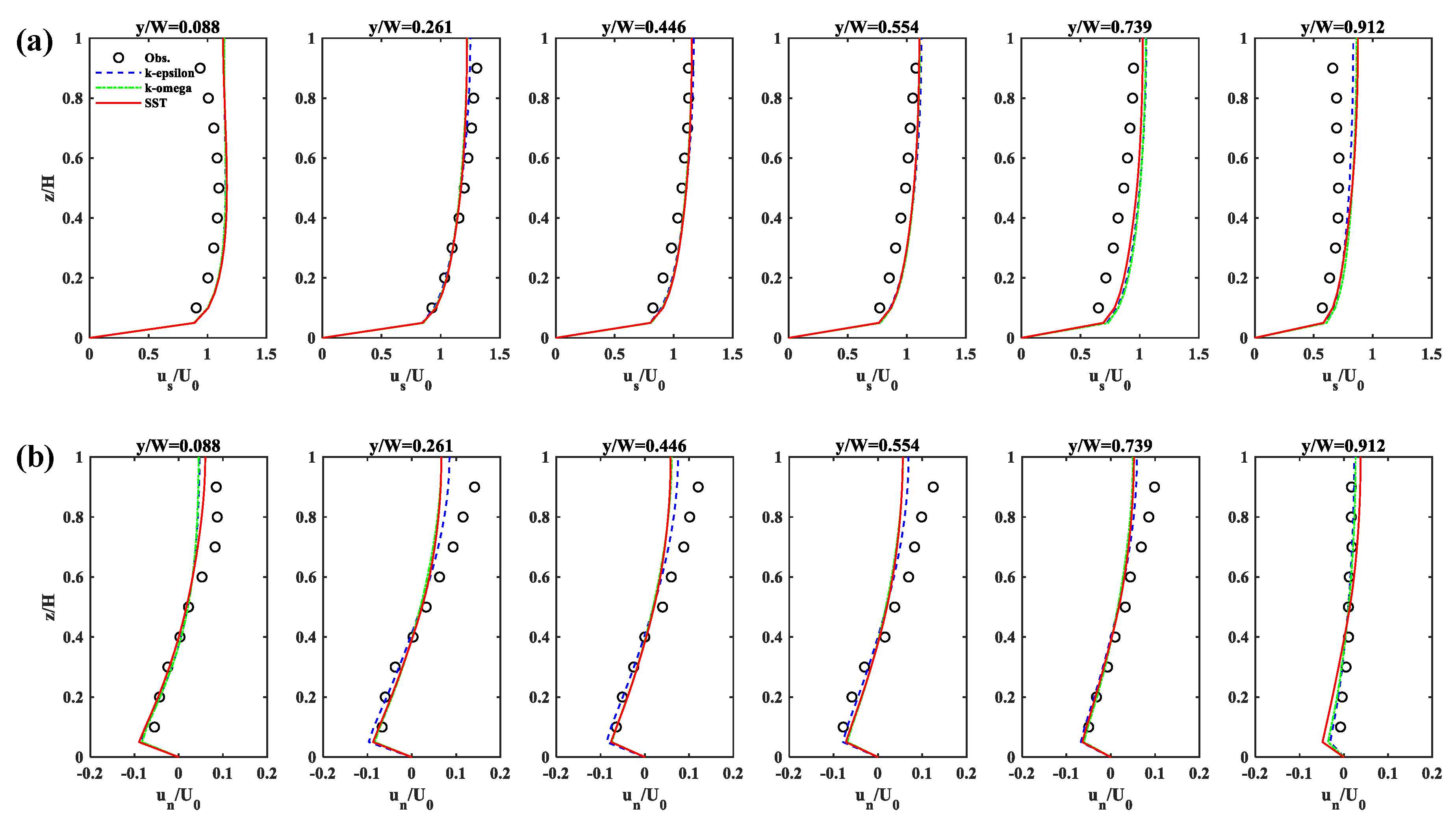
3.1. Velocity Distributions

This study explores 3D flow structures in meandering channels under the three different conditions of sinuosity. Figure 3 shows the mean velocity and turbulent kinetic energy (TKE) distributions simulated at the free surface with the SST $k-\omega$ model. In this figure, the mean velocity distributions exhibit that the maximum velocity develops near the inner bank due to the centrifugal force, while the minimum velocity evolves along the outer bank. This trend is contradictory to the velocity distribution in natural rivers because the generated channels have the flat and smooth bed [56,59]. In nature, rivers generally present the highest velocity along the outer bank because of sediment erosion and deposition. The significant velocity gradients in the transverse direction around the inlet of the meander bend increase TKE near the bend outlet because of a strong momentum transfer between the inner bank and the outer bank. As sinuosity increases, the discrepancy between the maximum inner-bank velocity and the minimum outer-bank velocity increases. Compared to S136 and S157, consequently, S190 exhibits the stronger velocity gradients across the channel width, which drive the higher level of TKE adjacent to the bend apex, as shown in Figure 3.

The momentum transfer within the meander bend is realized by the secondary flow. With the helical motion of the secondary flows, the high momentum fluid near the water surface transports toward the outer bank, whereas the low momentum fluid near the channel bed moves to the inner bank. The simulation results adequately reproduce these cross-sectional flow patterns, as depicted in Figure 4, in which the spanwise velocity vectors are overlain with the mean velocity distributions at the bend apex, simulated with three turbulence models under the different sinuosity conditions. This figure clearly shows that the secondary flow intensity is enhanced with increasing sinuosity, which also leads to an increase and a decrease in the velocity magnitude near the inner bank and the outer bank, respectively. All turbulence models used in this study successfully simulate the aforementioned helical secondary flows at the bend apex. Even if the entire flow features are consistent over all turbulence models, the SST $k-\omega$ model reproduces the stronger intensity of the secondary flow than that of the $k-\epsilon$ and $k-\omega$ models. Hence, the velocity near the water surface and channel bed, simulated with the SST $k-\omega$ model, are higher than that of other turbulence models.

The influence of the turbulence models on the flow simulations is investigated more rigorously using the depth-averaged streamwise velocity and width-averaged spanwise velocity profiles, as shown in Figure 5. From this figure, one can notice that the shear flows become stronger in both lateral and vertical directions as sinuosity increases. Although the topological characteristics exert a dominant control over the overall flow patterns in meandering channels, the detailed flow behaviors are governed by the turbulence models. In S136, the velocity profiles are barely sensitive to the turbulence models. In S190, in contrast, the SST $k-\omega$ model simulates the larger deviations in both the streamwise and spanwise velocity profiles than those of other turbulence models. Here, the transverse gradient of the streamwise velocity for $y/W<0.3$ near the outer bank increases more sharply with the SST $k-\omega$ model. The vertical profile of the spanwise velocity obtained from the SST $k-\omega$ model also shows the secondary flow to be stronger than that of other turbulence models. These results indicate that the SST $k-\omega$ model produces the stronger shear flows in the sharply curved meander bend compared to the $k-\epsilon$ and $k-\omega$ models. Therefore, the performance of the turbulence models may directly impact solute transport mechanisms related to the bulk shear dispersion as well as the turbulent diffusion.

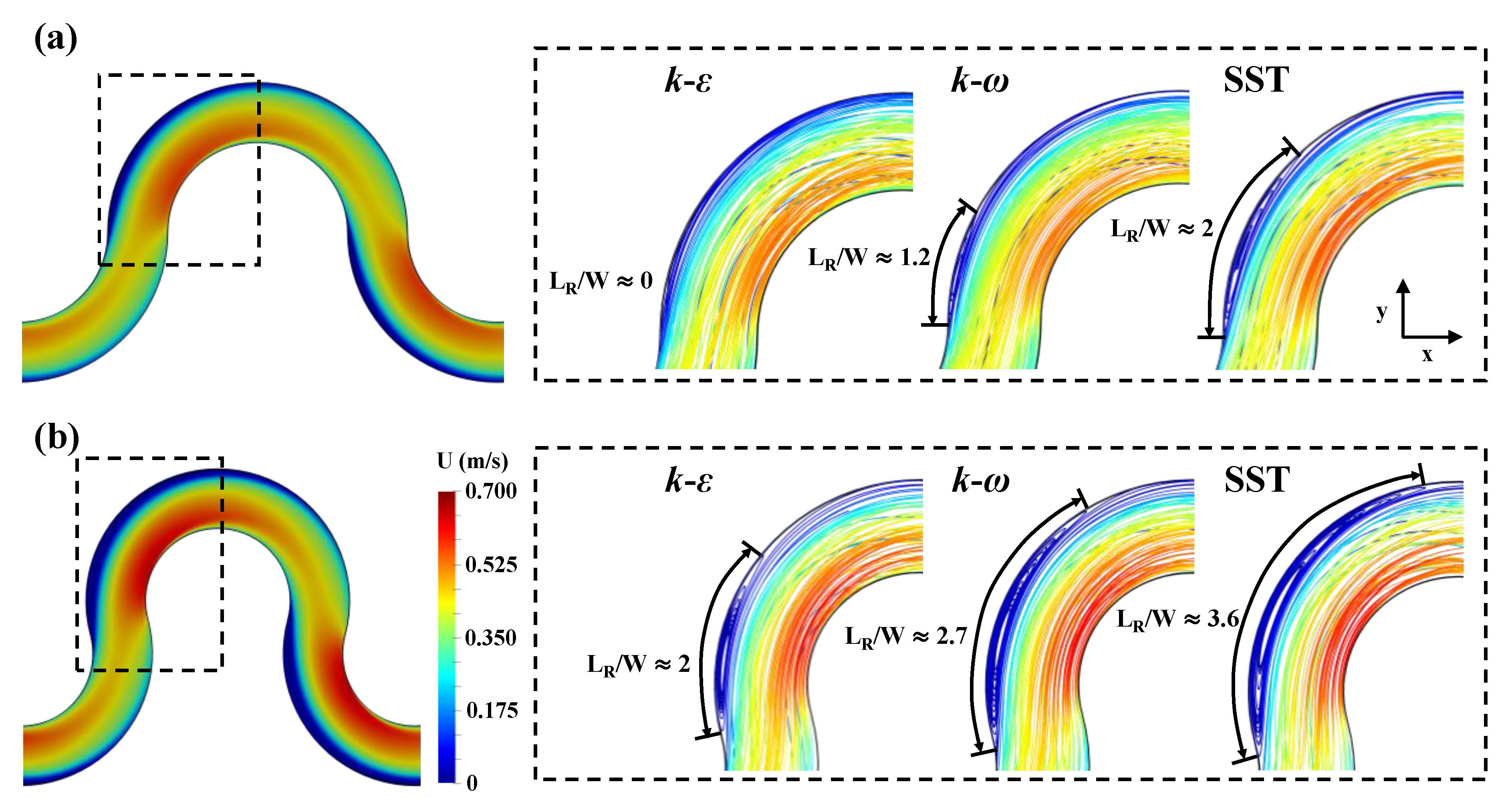
3.2. Separated Recirculating Flows

The high sinuosity causes the transverse gradient of the streamwise velocity biased largely toward the inner bank. This strong velocity gradient in the transverse direction forms the low-velocity zones near the outer bank, where it is notable that the negative streamwise velocity (backflow) is simulated at the bend apex with the SST $k-\omega$ model for S190, as shown in Figure 5a. From the backflow, it is evident that horizontal recirculating flows take place in the vicinity of the outer bank owing to the adverse pressure gradients associated with the sharp bend curvature. At high sinuosity, the streamwise velocity structures are substantially influenced by the turbulence models (Figure 5a). Thus, it can be inferred that the turbulence models may directly affect the recirculating flow characteristics.

Figure 6 shows that the separated recirculation zones emerge near the outer bank of the bend inlet in high-sinuosity cases of S157 and S190, as shown in Figure 6. Hickin [60] revealed that the onset of the horizontal flow separation occurs at a specific level of the curvature ratio to channel width, $R_c/W\le 2$, which is consistent with $R_c/W$ of S157 and S190, as presented in Table 1. According to Figure 6, however, the onset and size of the recirculation zones highly depend on the turbulence models. In S157, the $k-\omega$ and SST $k-\omega$ models adequately reproduce the onset of the recirculating flows, while the $k-\epsilon$ model fails to simulate the flow separation. In S190, all turbulence models are successful in reproducing the separated recirculating flows. Nevertheless, the $k-\epsilon$ and $k-\omega$ models unpredict the reattachment length of the flow separation for both S157 and S190 compared to the SST $k-\omega$ model (Figure 6).

The influence of the turbulence models on the flow separation is further examined using its width and velocity magnitude. The transverse distributions of the depth-averaged mean velocity at the cross-section across the center of the recirculation zones is plotted in Figure 7. With this figure, the width of the recirculation zones is implicitly estimated by measuring the distance between the center of the recirculation zone and the wall. Please note that this study assumes the minimum-velocity point other than the near-wall boundary as the center of the recirculation zone, as illustrated in Figure 7b. In S136, no flow recirculation is simulated with all turbulence models as the minimum velocity occurs very near the wall, as shown in Figure 7a. For S157 and S190, the SST $k-\omega$ model reproduces the faster and wider recirculating flows than those of other turbulence models, as depicted in Figure 7b,c. Particularly in S157, the $k-\epsilon$ model simulates the width of the recirculation zone close to zero, which indicates no occurrence of the flow separation (Figure 7b). These trends are consistent with the findings from Figure 6.

In the meandering channel studied in this work, the extent of the separated flow recirculation would be critical in quantifying the magnitude of the non-Fickian transport because the larger recirculation zones trap more solute particles and directly contribute to longer residence times of solutes. Additionally, the recirculating flow velocity may be significantly related to the trapping effects. The mass exchange between the main flow zone and the recirculation zone occurs via turbulent diffusion along the interface between the two different flow regimes, where the turbulent shear layer develops. Here, the fast recirculating flows suppress the solute diffusion from the recirculation zone into the main flow zone because of the strong inertial effects, thereby enhancing the trapping effects. As previously demonstrated, the onset, size, and velocity magnitude of the recirculating flows are considerably sensitive to the turbulence models. In consequence, it can be expected that the turbulence models control the non-Fickian transport behaviors simulated in the meandering channels.

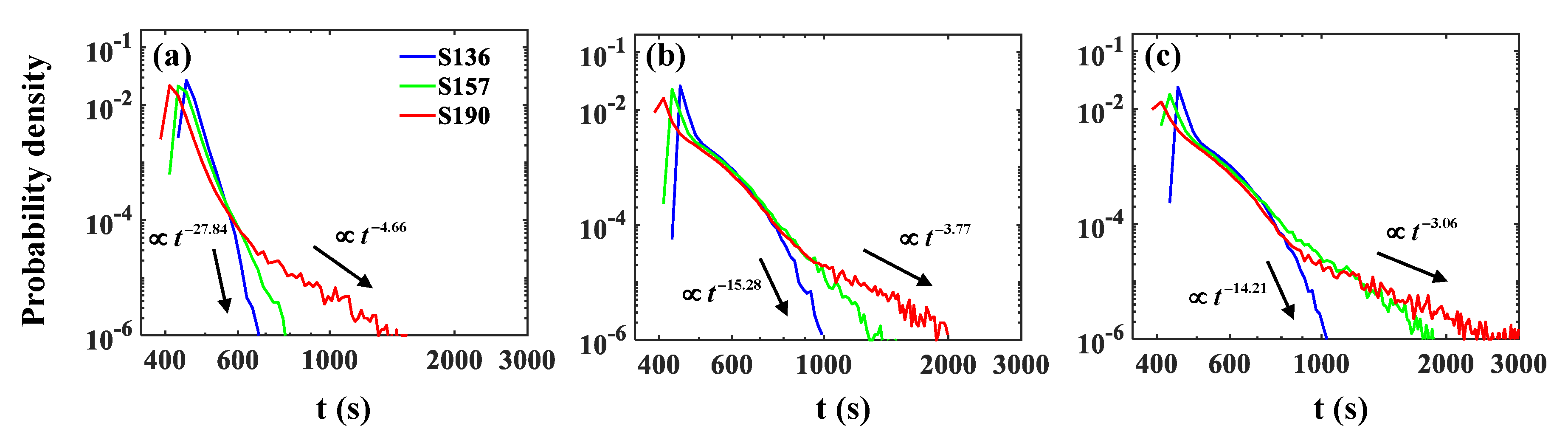
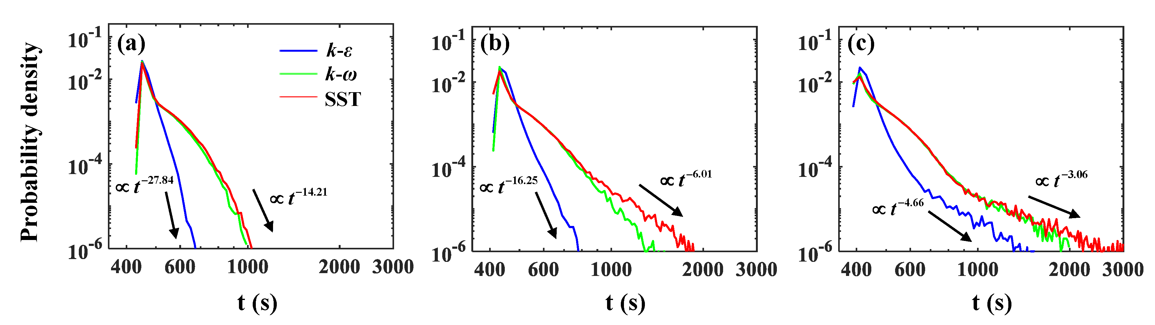
3.3. Solute Transport and Dispersion

For solute transport simulations, 2 × 10⁵ particles are instantaneously injected as a point source introduced from the center of the inlet cross-section, and the simulated mean velocity and turbulence fields at the steady state are used as input variables to govern advection and diffusion of the solute particles, respectively. The time step is set to retain Cr to be unity [7]. The effects of sinuosity on solute dispersion are first investigated. Figure 8 presents one-dimensional (1D) breakthrough curves (BTCs) at the channel outlet, simulated with the $k-\epsilon$, $k-\omega$ and SST $k-\omega$ models. This figure indicates probability density functions of particle residence times until they pass the outlet, which can conventionally be considered as particle residence time distributions. Herein, the probability density is calculated as the ratio of the number of particles, which pass the outlet at each measurement interval of 20 s (bin width of Figure 8), to the total particles of 2 × 10⁵ divided by the bin width. As shown in Figure 8, the longitudinal dispersion increases as sinuosity increases because the higher sinuosity leads to the larger elongation of the solute spreading in the streamwise direction, honoring the larger velocity gradients in the transverse direction. This trend is commonly observed in the BTCs simulated with all turbulence models. Yet, the tail scaling of the BTCs differ according to the turbulence models, as depicted in Figure 8. The scaling (slope) of the BTC tails is conventionally considered as a vital factor in quantifying the non-Fickian dispersion [61,62].

Figure 9 shows the impact of the turbulence models on the BTC tailing with a variation of channel sinuosity and demonstrates that the $k-\omega$ and SST $k-\omega$ models exhibit the heavier-tailed BTCs than those of the $k-\epsilon$ model. To quantify this disparity among the turbulence models, this study estimates the tail power-law slope and the truncation time, which are measures of the non-Fickian dispersion [41,61,62]. Here, the truncation time is defined as the ratio of the maximum residence time to the peak concentration time [57], and the power-law slope is calculated using the least-squares regression. Please note that the flatter power-law slope (smaller its absolute value) and larger truncation time characterize the stronger non-Fickian dispersion with the heavier BTC tailing. The power-law slope and truncation time for all simulation cases are summarized in

Table 2. Key parameters of breakthrough curves to evaluate the impact of turbulence models on tailing behaviors of solute particle spreading.

Model	S136		S157		S190
	Tail Power-Law Slope	Truncation Time	Tail Power-Law Slope	Truncation Time	Tail Power-Law Slope	Truncation Time
$k-\epsilon$	−27.84	1.49	−16.25	1.81	−4.66	3.54
$k-\omega$	−15.28	2.20	−7.68	3.19	−3.77	4.85
SST	−14.21	2.29	−6.01	4.30	−3.06	6.32

. In S136, the $k-\epsilon$ model exhibits the steeper power-law slope and smaller truncation time than those of other turbulence models since this turbulence model simulates the relatively smaller transverse gradient of the mean velocity (weaker shear-flow effect), as shown in Figure 7a. According to Figure 9, this tendency is more pronounced in higher-sinuosity cases of S157 and S190. As sinuosity increases to 1.57 from 1.36, the power-law slope and truncation time ratios of the $k-\epsilon$ model to the SST $k-\omega$ model increase and decrease to 2.70 and 0.42 from 1.96 and 0.65, respectively, as presented in Table 2. Besides, S157 shows that the SST $k-\omega$ model yields the larger truncation time and flatter power-law slope than those of the $k-\omega$ model even though no significant difference in the BTC parameters between these two turbulence models is found in S136.

The occurrence of the separated flow recirculation can explain the increasing discrepancy in the BTC parameters between the turbulence models, corresponding to increasing sinuosity. In S136, no flow separation is simulated with all turbulence models (Figure 7a). Thus, the difference in the BTC shape among the turbulence models is purely driven by the difference in the shear flow effects determined by the transverse gradients of the mean velocity, as shown in Figure 10a. In S157, meanwhile, the $k-\omega$ and SST $k-\omega$ models reproduce the flow separation in the vicinity of the outer bank (Figure 6a). This separated flow traps solute particles to the outer bank via the recirculating flows, then enhance the late-time tailing, as demonstrated in Figure 10b. As a result, the remarkable change in the BTC parameters between S136 and S157 is observed with the $k-\omega$ and SST $k-\omega$ models due to the trapping effects of the flow separation. More specifically, the SST $k-\omega$ model exhibits that the absolute value of the power-law slope, and truncation time of S157 are about half and twice the values of S136, respectively (Table 2). On the other hand, the $k-\epsilon$ model fails to predict the onset of the flow separation for S157. The absence of the trapping effects caused by the flow separation induces the minor difference in the BTC shape between S136 and S157 with the $k-\epsilon$ model (Figure 9a,b). In S190, the onset of the separated recirculating flows is successfully simulated with all turbulence models even though the size of the recirculation zone varies with the turbulence models (Figure 6b). As a consequence, the $k-\epsilon$ model shows the sudden change in the BTC shape between S157 and S190, wherein the absolute value of the power-law slope, and truncation time of S190 are about one-third and twice the values of S157, respectively (Table 2). Moreover, the discrepancy in the power-law slope among the turbulence models is considerably reduced in S190.

According to Table 2, the simulation cases involving the recirculating flows commonly have truncation times larger than 3. This result implies that this truncation time value can be suggested as the threshold for identifying the non-Fickian transport signature ascribed to the flow separation in the meandering channels of this study. Nevertheless, the $k-\epsilon$ and $k-\omega$ models exhibit the smaller truncation times and steeper power-law slopes than those of the SST $k-\omega$ model. As previously discussed, this is because the reattachment length, width, and velocity magnitude of the recirculation zones differ by different turbulence models. Compared to the $k-\epsilon$ and $k-\omega$ models, the SST $k-\omega$ reproduces the larger and faster recirculating flows (Figure 6 and Figure 7), and thus exacerbates the late-time tailing of the BTCs (Figure 9) owing to the stronger storage (trapping) effects on solute transport, as visualized in Figure 10c. Furthermore, the enhanced secondary flows simulated with the SST $k-\omega$ model (Figure 5b) may promote the trapping effects by vigorously conveying solute particles to the flow separation zones near the outer bank via the transverse dispersion. Therefore, the turbulence models significantly affect the solute transport simulations in meandering-open channel flows since these turbulence closure schemes govern the separated recirculating flow and secondary flow structures directly controlling the non-Fickian transport behaviors.

4. Conclusions

This study quantified the influence of turbulence closure models in simulating curvature-driven flow separation and resulting non-Fickian mixing behaviors in meandering open channels across a wide range of sinuosity. To achieve this task, the 3D RANS equations integrated with $k-\epsilon$, $k-\omega$ and SST $k-\omega$ turbulence models were used for flow simulations, and the 3D LPT model was adopted for solute transport simulations. The major findings from this work can be summarized as:

• The strong transverse gradients of mean velocity simulated with increasing sinuosity induce the flow separation along the outer bank for channel sinuosity 1.57 and 1.90 because of the adverse pressure gradients. The size of the flow separation increases as sinuosity increases.
• The onset and size of the flow separation are significantly affected by the turbulence models. Notably, the $k-\epsilon$ model fails to predict the emergence of the flow separation or unpredicts its reattachment length and width by underestimating the velocity gradients.
• The flow separation with vigorous recirculating flows acts as a storage (trapping) zone of solute particles, and the trapping effects increase solute residence times. Here, the $k-\epsilon$ model underestimates the power-law tailing of BTCs since it undervalues the effects of the separated flow recirculation compared to the other turbulence models.
• The SST $k-\omega$ model yields heavier-tailed BTCs characterized by flatter power-law slopes and larger truncation times as it reproduces larger and faster recirculating flows than the $k-\epsilon$ and $k-\omega$ models.

Consequently, the present work elucidated that the turbulence models substantially impact the 3D solute transport simulations since these turbulence closure schemes determine the onset and extent of the separated flow recirculation identified as the surface storage zones. Even if the 3D model is effective in explicitly understanding the interaction between solute dispersion and hydrodynamic effects, this approach may not be appropriate for water quality management in rivers and streams because of the high computational demand. Therefore, the next stage of this study will parameterize the transient storage model, which is the 1D upscaled model extensively used for simulating the non-Fickian transport in rivers and streams [63], using the simulation results of this work and predict the heavy-tailed BTCs induced by the meander-driven flow separation.

References

1. Johannesson, H.; Parker, G. Secondary flow in mildly sinuous channel. J. Hydraul. Eng. 1989, 115, 289–308. [Google Scholar] [CrossRef]
2. Blanckaert, K.; de Vriend, H.J. Nonlinear modeling of mean flow redistribution in curved open channels. Water Resour. Res. 2003, 39. [Google Scholar] [CrossRef]
3. Marion, A.; Zaramella, M. Effects of velocity gradients and secondary flow on the dispersion of solutes in a meandering channel. J. Hydraul. Eng. 2006, 132, 1295–1302. [Google Scholar] [CrossRef]
4. Boxall, J.B.; Guymer, I. Analysis and prediction of transverse mixing coefficients in natural channels. J. Hydraul. Eng. 2003, 129, 129–139. [Google Scholar] [CrossRef]
5. Baek, K.O.; Seo, I.W.; Jeong, S.J. Evaluation of dispersion coefficients in meandering channels from transient tracer tests. J. Hydraul. Eng. 2006, 132, 1021–1032. [Google Scholar] [CrossRef]
6. Davis, P.M.; Atkinson, T.C.; Wigley, T.M.L. Longitudinal dispersion in natural channels: 2. The roles of shear flow dispersion and dead zones in the River Severn, UK. Hydrol. Earth Syst. Sci. 2000, 4, 355–371. [Google Scholar] [CrossRef] [Green Version]
7. Park, I.; Seo, I.W. Modeling non-Fickian pollutant mixing in open channel flows using two-dimensional particle dispersion model. Adv. Water Resour. 2018, 111, 105–120. [Google Scholar] [CrossRef]
8. Rameshwaran, P.; Nade, P.S. Three-dimensional modelling of free surface variation in a meandering channel. J. Hydraul. Res. 2004, 42, 603–615. [Google Scholar] [CrossRef]
9. Wormleaton, P.R.; Ewunetu, M. Three-dimensional k-ε numerical modelling of overbank flow in a mobile bed meandering channel with floodplains of different depth, roughness and planform. J. Hydraul. Res. 2006, 44, 18–32. [Google Scholar] [CrossRef]
10. Fischer-Antze, T.; Ruther, N.; Olsen, N.R.B.; Gutknecht, D. Three-dimensional (3D) modeling of non-uniform sediment transport in a channel bend with unsteady flow. J. Hydraul. Res. 2009, 47, 670–675. [Google Scholar] [CrossRef]
11. Rüther, N.; Olsen, N.R.B. Three-dimensional modeling of sediment transport in a narrow 90° channel bend. J. Hydraul. Eng. 2005, 131, 917–920. [Google Scholar] [CrossRef]
12. Stoesser, T.; Ruether, N.; Olsen, N.R.B. Calculation of primary and secondary flow and boundary shear stresses in a meandering channel. Adv. Water Resour. 2010, 33, 158–170. [Google Scholar] [CrossRef]
13. Van Balen, W.; Blanckaert, K.; Uijttewaal, W.S.J. Analysis of the role of turbulence in curved open-channel flow at different water depths by means of experiments, LES and RANS. J. Turbul. 2010, 11, 1–34. [Google Scholar] [CrossRef]
14. Farhadi, A.; Sindelar, C.; Tritthart, M.; Glas, M.; Blanckaert, K.; Habersack, H. An investigation on the outer bank cell of secondary flow in channel bends. J. Hydro-Environ. Res. 2018, 18, 1–11. [Google Scholar] [CrossRef]
15. Russell, P.; Vennell, R. High resolution observations of an outer-bank cell of secondary circulation in a natural river bend. J. Hydraul. Res. 2019, 145, 04019012. [Google Scholar] [CrossRef]
16. Demuren, A.O.; Rodi, W. Calculation of flow and pollutant dispersion in meandering channels. J. Fluid Mech. 1986, 172, 63–92. [Google Scholar] [CrossRef]
17. Ye, J.; McCorquodale, J.A. Simulation of curved open channel flows by 3D hydrodynamic model. J. Hydraul. Eng. 1998, 124, 687–698. [Google Scholar] [CrossRef]
18. Ferguson, R.I.; Parsons, D.R.; Lane, S.N.; Hardy, R.J. Flow in meander bends with recirculation at the inner bank. Water Resour. Res. 2003, 39. [Google Scholar] [CrossRef] [Green Version]
19. Abad, J.D.; Frias, C.E.; Buscaglia, G.C.; Garcia, M.H. Modulation of the flow structure by progressive bedforms in the Kinoshita meandering channel. Earth Surf. Process. Landf. 2013, 38, 1612–1622. [Google Scholar] [CrossRef]
20. Rameshwaran, P.; Naden, P.; Wilson, C.A.; Malki, R.; Shukla, D.R.; Shiono, K. Inter-comparison and validation of computational fluid dynamics codes in two-stage meandering channel flows. Appl. Math. Model. 2013, 37, 8652–8672. [Google Scholar] [CrossRef] [Green Version]
21. Argyropoulos, C.D.; Markatos, N.C. Recent advances on the numerical modelling of turbulent flows. Appl. Math. Model. 2015, 39, 693–732. [Google Scholar] [CrossRef]
22. Wilcox, D.C. Formulation of the k-ω turbulence model revisited. AIAAJ J. 2008, 46, 2823–2838. [Google Scholar] [CrossRef] [Green Version]
23. El-Behery, S.M.; Hamed, M.H. A comparative study of turbulence models performance for separating flow in a planar asymmetric diffuser. Comput. Fluids 2011, 44, 248–257. [Google Scholar] [CrossRef]
24. Khosronejad, A.; Rennie, C.D.; Salehi Neyshabouri, S.A.A.; Townsend, R.D. 3D numerical modeling of flow and sediment transport in laboratory channel bends. J. Hydraul. Eng. 2007, 133, 1123–1134. [Google Scholar] [CrossRef]
25. Menter, F.R. Two-equation eddy-viscosity turbulence models for engineering applications. AIAA J. 1994, 32, 1598–1605. [Google Scholar] [CrossRef] [Green Version]
26. Sparrow, E.M.; Abraham, J.P.; Minkowycz, W.J. Flow separation in a diverging conical duct: Effect of Reynolds number and divergence angle. Int. J. Heat Mass Transf. 2009, 52, 3079–3083. [Google Scholar] [CrossRef]
27. Luo, H.; Fytanidis, D.K.; Schmidt, A.R.; García, M.H. Comparative 1D and 3D numerical investigation of open-channel junction flows and energy losses. Adv. Water Resour. 2018, 117, 120–139. [Google Scholar] [CrossRef]
28. Nguyen, T.H.T.; Ahn, J.; Park, S.W. Numerical and physical investigation of the performance of turbulence modeling schemes around a scour hole downstream of a fixed bed protection. Water 2018, 10, 103. [Google Scholar] [CrossRef] [Green Version]
29. Khosronejad, A.; Hansen, A.T.; Kozarek, J.L.; Guentzel, K.; Hondzo, M.; Guala, M.; Wilcock, P.R.; Finlay, J.C. Large eddy simulation of turbulence and solute transport in a forested headwater stream. J. Geophys. Res. Earth Surf. 2016, 121, 146–167. [Google Scholar] [CrossRef] [Green Version]
30. Kim, J.S.; Baek, D.; Seo, I.W.; Shin, J. Retrieving shallow stream bathymetry from UAV-assisted RGB imagery using a geospatial regression method. Geomorphology 2019, 341, 102–114. [Google Scholar] [CrossRef]
31. Blanckaert, K. Topographic steering, flow recirculation, velocity redistribution, and bed topography in sharp meander bends. Water Resour. Res. 2010, 46. [Google Scholar] [CrossRef]
32. Blanckaert, K. Hydrodynamic processes in sharp meander bends and their morphological implications. J. Geophys. Res. Earth Surf. 2011, 116. [Google Scholar] [CrossRef] [Green Version]
33. Blanckaert, K.; Kleinhans, M.G.; McLelland, S.J.; Uijttewaal, W.S.; Murphy, B.J.; van de Kruijs, A.; Parsons, D.R.; Chen, Q. Flow separation at the inner (convex) and outer (concave) banks of constant-width and widening open-channel bends. Earth Surf. Process. Landf. 2013, 38, 696–716. [Google Scholar] [CrossRef] [Green Version]
34. Jackson, T.R.; Haggerty, R.; Apte, S.V.; Coleman, A.; Drost, K.J. Defining and measuring the mean residence time of lateral surface transient storage zones in small streams. Water Resour. Res. 2012, 48. [Google Scholar] [CrossRef] [Green Version]
35. Sandoval, J.; Mignot, E.; Mao, L.; Pastén, P.; Bolster, D.; Escauriaza, C. Field numerical investigation of transport mechanisms in a surface storage zone. J. Geophys. Res. Earth Surf. 2019, 124, 938–959. [Google Scholar] [CrossRef] [Green Version]
36. Wilson, C.A.M.E.; Guymer, I.; Boxall, J.B.; Olsen, N.R.B. Three-dimensional numerical simulation of solute transport in a meandering self-formed river channel. J. Hydraul. Res. 2007, 45, 610–616. [Google Scholar] [CrossRef]
37. Zhang, M.L.; Li, C.W.; Shen, Y.M. A 3D non-linear k-ε turbulent model for prediction of flow and mass transport in channel with vegetation. Appl. Math. Model. 2010, 34, 1021–1031. [Google Scholar] [CrossRef]
38. Liu, X.; García, M.H. Three-dimensional numerical model with free water surface and mesh deformation for local sediment scour. J. Waterw. Port Coast. Ocean Eng. 2008, 134, 203–217. [Google Scholar] [CrossRef]
39. Bayon-Barrachina, A.; Lopez-Jimenez, P.A. Numerical analysis of hydraulic jumps using OpenFOAM. J. Hydroinform. 2015, 17, 662–678. [Google Scholar] [CrossRef] [Green Version]
40. Bayon, A.; Valero, D.; García-Bartual, R.; Vallés-Morán, F.J. Performance assessment of OpenFOAM and FLOW-3D in the numerical modeling of a low Reynolds number hydraulic jump. Environ. Model. Softw. 2016, 80, 322–335. [Google Scholar] [CrossRef]
41. Hromadka, T.V., II; Rao, P. Examination of computational precision versus modeling complexity for open channel flow with hydraulic jump. J. Water Resour. Prot. 2019, 11, 1233–1244. [Google Scholar]
42. Wang, Y.; Politano, M.; Laughery, R.; Weber, L. Model development in OpenFOAM to predict spillway jet regimes. J. Appl. Water Eng. Res. 2015, 3, 80–94. [Google Scholar] [CrossRef]
43. Duguay, J.M.; Lacey, R.W.J.; Gaucher, J. A case study of a pool and weir fishway modeled with OpenFOAM and FLOW-3D. Ecol. Model. 2017, 103, 31–42. [Google Scholar] [CrossRef]
44. Bayon, A.; Toro, J.P.; Bombardelli, F.A.; Matos, J.; López-Jiménez, P.A. Influence of VOF technique, turbulence model and discretization scheme on the numerical simulation of the non-aerated, skimming flow in stepped spillways. J. Hydro-Environ. Res. 2018, 19, 137–149. [Google Scholar] [CrossRef] [Green Version]
45. Kim, J.S.; Kang, P.K. Anomalous transport through free-flow-porous media interface: Pore-scale simulation and predictive modeling. Adv. Water Resour. 2020, 135, 103467. [Google Scholar] [CrossRef]
46. Jones, W.P.; Launder, B.E. The prediction of laminarization with a two-equation model of turbulence. Int. Heat Mass Transfer. 1972, 15, 301–314. [Google Scholar] [CrossRef]
47. Pope, S.B. Turbulent Flows; Cambridge University Press: Cambridge, UK, 2000; pp. 373–384. [Google Scholar]
48. Zeng, J.; Constantinescu, G.; Weber, L. A 3D non-hydrostatic model to predict flow and sediment transport in loose-bed channel bends. J. Hydraul. Res. 2008, 46, 56–372. [Google Scholar] [CrossRef]
49. Kang, S.; Lightbody, A.; Hill, C.; Sotiropoulos, F. High-resolution numerical simulation of turbulence in natural waterways. Adv. Water Resour. 2011, 34, 98–113. [Google Scholar] [CrossRef]
50. Kang, S.; Sotiropoulos, F. Numerical modeling of 3D turbulent free surface flow in natural waterways. Adv. Water Resour. 2012, 40, 23–36. [Google Scholar] [CrossRef]
51. Gosman, A.D.; Loannides, E. Aspects of computer simulation of liquid-fueled combustors. J. Energy 1983, 7, 482–490. [Google Scholar] [CrossRef]
52. Shams, M.; Ahmadi, G.; Smith, D.H. Computational modeling of flow and sediment transport and deposition in meandering rivers. Adv. Water Resour. 2002, 25, 689–699. [Google Scholar] [CrossRef]
53. Dehbi, A. Turbulent particle dispersion in arbitrary wall-bounded geometries: A coupled CFD-Langevin-equation based approach. Int. J. Multiph. Flow 2008, 34, 819–828. [Google Scholar] [CrossRef]
54. Rybalko, M.; Loth, E.; Lankford, D.A. Lagrangian particle random walk model for hybrid RANS/LES turbulent flows. Powder Technol. 2012, 221, 105–113. [Google Scholar] [CrossRef]
55. Hey, R.D. Geometry of river meanders. Nature 1976, 262, 482. [Google Scholar] [CrossRef]
56. Chang, Y.C. Lateral mixing in meandering channels. In River Meandering; ASCE: Reston, VA, USA, 1971; pp. 598–610. [Google Scholar]
57. Hodskinson, A.; Ferguson, R.I. Numerical modelling of separated flow in river bends: Model testing and experimental investigation of geometric controls on the extent of flow separation at the concave bank. Hydrol. Process. 1998, 12, 1323–1338. [Google Scholar] [CrossRef]
58. Vinuesa, R.; Schlatter, P.; Nagib, H.M. Secondary flow in turbulent ducts with increasing aspect ratio. Phys. Rev. Fluids 2018, 3, 054606. [Google Scholar] [CrossRef]
59. Abad, J.D.; Garcia, M.H. Experiments in a high-amplitude Kinoshita meandering channel: 1. Implications ooi:f bend orientation on mean and turbulent flow structure. Water Resour. Res. 2009, 45. [Google Scholar] [CrossRef] [Green Version]
60. Hickin, E.J. Mean flow structure in meanders of the Squamish River, British Columbia. Can. J. Earth Sci. 1978, 15, 1833–1849. [Google Scholar] [CrossRef] [Green Version]
61. Aubeneau, A.F.; Hanrahan, B.; Bolster, D.; Tank, J.L. Substrate size and heterogeneity control anomalous transport in small streams. Geophys. Res. Lett. 2014, 41, 8335–8341. [Google Scholar] [CrossRef]
62. Drummond, J.D.; Covino, T.P.; Aubeneau, A.F.; Leong, D.; Patil, S.; Schumer, R.; Packman, A.I. Effects of solute breakthrough curve tail truncation on residence time estimates: A synthesis of solute tracer injection studies. J. Geophys. Res. Biogeosci. 2012, 117. [Google Scholar] [CrossRef] [Green Version]
63. Runkel, R.L.; Chapra, S.C. An efficient numerical solution of the transient storage equations for solute transport in small streams. Water Resour. Res. 1993, 29, 211–215. [Google Scholar] [CrossRef]
Figure 1. Channel geometries generated by Hey’s relations and corresponding computational grids for simulation cases with different sinuosity levels.
Applsci 10 02769 g001
Figure 2. Comparison between observation of Chang’s experiments and simulations with three turbulence models: (a) streamwise velocity profiles and (b) spanwise velocity profiles. y / W and z / H denote the dimensionless distance from the left bank and channel bed, respectively.
Applsci 10 02769 g002
Figure 3. Mean velocity and turbulence fields at the free surface of a representative domain including the bend apex for simulation cases calculated with the SST k ω model.
Applsci 10 02769 g003
Figure 4. Cross-sectional distributions of mean velocity with secondary flows at the bend apex for simulation cases with three different turbulence models.
Applsci 10 02769 g004
Figure 5. Influence of turbulence models on distributions of (a) depth-averaged streamwise velocity and (b) width-averaged spanwise velocity at the bend apex for S136 and S190. The insets indicate streamwise and spanwise velocity distributions of the SST k ω model, as a function of sinuosity.
Applsci 10 02769 g005
Figure 6. Streamlines of velocity fields for (a) S157 and (b) S190, simulated with different turbulence models. L R indicates the reattachment length of recirculation zones.
Applsci 10 02769 g006
Figure 7. Distributions of depth-averaged mean velocity at the cross-section crossing the center of recirculation zones for (a) S136, (b) S157, and (c) S190. The insets plot the distributions with the logarithmic scale on y-axis.
Applsci 10 02769 g007
Figure 8. 1D breakthrough curves of S136, S157, and S190, in which particle residence times are measured at the channel outlet, simulated with (a) the k ε model, (b) the k ω model, and (c) the SST k ω model.
Applsci 10 02769 g008
Figure 9. Impact of turbulence models on 1D breakthrough curves of (a) S136, (b) S157, and (c) S190.
Applsci 10 02769 g009
Figure 10. Particle positions for (a) S136, (b) S157, and (c) S190 at t = 500 s, simulated with the 3D LPT model based on flow fields obtained from the k ε model and SST k ω model. The colormap indicates Lagrangian velocity of particles.
Applsci 10 02769 g010