Article

Robust Structural Damage Detection Using Analysis of the CMSE Residual’s Sensitivity to Damage

1
Shandong Provincial Key Laboratory of Ocean Engineering, Ocean University of China, Qingdao 266100, China
2
Department of Port and Waterway Engineering, College of Civil Engineering, Ludong University, Yantai 264000, China
*
Author to whom correspondence should be addressed.
Appl. Sci. 2020, 10(8), 2826; https://doi.org/10.3390/app10082826
Submission received: 28 March 2020 / Revised: 12 April 2020 / Accepted: 16 April 2020 / Published: 19 April 2020
(This article belongs to the Special Issue Novel Approaches for Structural Health Monitoring)

Abstract

:
This paper presents a robust damage identification scheme in which damage is predicted by solving the cross-modal strain energy (CMSE) linear system of equations. This study aims to address the excessive equations issue faced in the assemblage of the CMSE system. A sensitivity index that, to some extent, measures how the actual damage level vector satisfies each CMSE equation, is derived by performing an analysis of the defined residual’s sensitivity to damage. The index can be used to eliminate redundant equations and enhance the robustness of the CMSE system. Moreover, to circumvent a potentially ill-conditioned problem, a previously published iterative Tikhonov regularization method is adopted to solve the CMSE system. Some improvements to this method for determining the iterative regularization parameter and regularization operator are given. The numerical robustness of the proposed damage identification scheme against measurement noise is proved by analyzing a 2-D truss structure. The effects of location and extent of damage on the damage identification results are investigated. Furthermore, the feasibility of the proposed scheme for damage identification is experimentally validated on a beam structure.

1. Introduction

Structural damage identification is a fundamental element of structural health monitoring (SHM) that has become a vital tool in maintaining the safety and integrity of structures [1,2,3,4,5,6,7]. Research on vibration-based damage identification has been rapidly expanding over recent decades. The basic idea behind this technology is that modal parameters (notably frequencies, mode shapes, and modal damping) are functions of the physical properties of the structure. Therefore, changes in the physical properties (such as stiffness reduction caused by damage) will cause detectable changes in the modal properties. Conversely, these changes can be used to reflect damage.
Vibration-based structural damage identification can be formulated as a linear inverse problem [8,9,10,11,12], which requires the determination of the unknown input (i.e., structural damage) to a linear system from the known output (i.e., extracted modal parameters from the vibration measurements of the structure). The discretization of the linear inverse problem [12,13] typically gives rise to the linear system of equations with a very ill-conditioned matrix C * [14],
C * α = b * ,   C * N q × N d ,   α N d ,   b * N q ,
where the coefficient matrix C * and the right-hand side vector b * are both assembled by the identified modal parameters and will be given in Equation (16); α is the unknown damage level vector to be solved, whose definition will be given in Equation (13); and the superscript “*” indicates a damaged version of physical or modal parameters. In other words, these parameters are dependent on α ; and N q and N d are the number of linear equations in the system and the potentially damaged elements, respectively. Usually, N q N d is required to ensure that the linear system of equations has a unique solution. In general, the computation of a meaningful approximate solution of the linear system requires that the system be replaced by a nearby system that is less sensitive to perturbations. This replacement is referred to as regularization. Tikhonov regularization is one of the most popular regularization techniques that can damp out the small measurement errors and single out a relatively accurate solution [15]. So far, it has been widely applied to damage detection [16,17,18] and other related research, such as model updating [19,20] and load identification [21]. Björck [22] gave a general form of Tikhonov regularization as follows:
( C * T C * + ξ 2 L T L ) α = C * T b *
where ξ 2 and L are the regularization parameter and the regularization operator, respectively. Then, the solution α of Equation (2) satisfies the minimization problem
min α N d { C * α b * 2 + ξ 2 L α 2 }
Here and below, · denotes the Euclidean norm. The determination of a suitable value of ξ 2 and L is an important task. In many previously developed methods, ξ 2 is selected using an L-curve criterion [12,15] or the generalized cross-validation method [20,23], but both methods are time-consuming computational tasks. Besides, the regularization parameter L is usually selected as an identity operator and thus leads to over-smoothing of the solution, which goes against the sparse feature of isolated damage at the early stage of structural deterioration [18]. Wang et al. [24] proposed the iterative Tikhonov regularization (ITR) method specialized for the identification of the isolated damage to structures. The method has some advantages, including the incorporation of an adaptive strategy to simultaneously determine ξ 2 and L . Additionally, the ITR method shows good convergence behavior.
Over the past decades, numerous techniques for damage identification have been reported. Carden and Fanning [25] gave a review of vibration-based condition monitoring that revealed numerous and diverse algorithms using data in the time, frequency, and modal domains. Yan et al. [26] presented a general summary of the state-of-art of intelligent algorithms, and their application prospects in structural damage identification were introduced. Among many reviews of the existing literature concerning damage identification methods, Fan and Qiao [27] dealt in particular with the subset of methods related to variations in basic modal properties. Changes or lack of smoothness in mode shape or mode shape curvature, analysis of dynamically measured flexibility, and updating of structural model parameters provide different examples of this family of methods. Dessi and Camerlengo [28] also focused on technique processing information about mode shape curvature or strain modes with or without knowledge of baseline data. The general modal strain energy (MSE), as an extension of mode shape analysis, is widely appreciated because of its excellent damage-sensitive features [29,30]. It is formed by the product of the stiffness matrix and the second power of mode shape:
P j , n * = ( ϕ j * ) T K n * ϕ j *   ( j = 1 , 2 , , N j )
where N j is the number of measured modes; ϕ j * and K n * are the j-th mode shape and the n-th stiffness submatrix of the damaged structure, respectively; and P j , n * is the MSE of the n-th damaged structural element associated with the j-th measured mode. When damage occurs, the distribution of strain energy originally stored in the structure will change in a more pronounced manner in the detected areas. Therefore, changes in the modal strain energy distributions of the healthy and damaged structures can be used to detect the existence, location, and extent of the damage. A review of MSE-based methods was given by Wang and Xu [29], and will not be discussed here.
In this study, a special MSE method named the CMSE method, proposed by Hu et al. [10] and later improved by Wang et al. [31], is used for damage detection. The adjective “cross” here indicates that MSE-like terms are product terms extending over the baseline finite element model (FEM) of the healthy structure and the measured damaged structure, also extending over various modes. The CMSE is defined as
C m , n * = ( ϕ i ) T K n ϕ j *   ( i = 1 , 2 , , N i ,   j = 1 , 2 , , N j )
where ϕ i and K n are the i-th analytical mode shape and the n-th stiffness submatrix of the baseline FEM, respectively, and N i is the number of analytical modes. In practice, it is easy to obtain the analytical modes of the baseline FEM, but difficult or expensive to extract the measured modes of the damaged structure [10]; therefore, one may select a much larger N i than N j , i.e., N i N j .
It is clear that the CMSE does not require matching modes between the healthy and damaged structures, and thus has more available mode combinations (MCs) than the general MSE, i.e., N i × N j N j . Like many other damage identification techniques, the CMSE method can establish a linear system of the same number of equations as the available measured mode or MCs. Therefore, a distinct advantage of this method is that it breaks through the constraint that the number of available measured modes is smaller than that of actual damages, i.e., N j < N d . It further raises the possibility that one can assume all N e   ( N e N d ) structural elements are damaged in case of omitting any actual damage only if sufficient equations ( N i × N j N e ) are constructed. Nevertheless, the disadvantages of constructing excessive equations are obvious. On the one hand, the damage identification result by solving a linear system assembled by different equations varies, leading to complicated decisions surrounding the actual damage state of the structure. On the other hand, the redundant equations do not contribute to damage detection but complicate the system, and exacerbate the damage identification result.
The main purpose of this study is to address the excessive equations issue faced in the assemblage of the CMSE linear system of equations. From the standpoint of solving a linear system of equations, optimizing the assemblage of the system by eliminating redundant equations serves as an effective tool to improve identification of damage, which has been rarely investigated in previous research. The ITR method is adopted as a tool for solving the linear system of equations given by Equation (1), with some improvements to this method also presented. This study contributes towards supplying a guideline for the elimination of the redundant equations to enhance the robustness of the CMSE system. A sensitivity index that, to some extent, measures how the actual damage level vector satisfies each CMSE equation is derived by performing an analysis of the defined residual’s sensitivity to damage. Finally, the numerical and experimental robustness of the proposed damage identification scheme against measurement noise is investigated.

2. Theoretical Background

2.1. CMSE Method

If M , K and M * , K * are used to denote the mass and stiffness matrices for baseline FEM of the healthy structure and the measured damaged structure, respectively, the following can be written:
K ϕ i = λ i M ϕ i
K * ϕ j * = λ j * M * ϕ j *
where λ i and λ j * are the i-th and the j-th eigenvalue of the baseline FEM of the healthy structure and the measured damaged structure, respectively.
The CMSE method is developed under the assumption that the mass distributions of the healthy and damaged structures are not known, but do not change, that is M * = M . In the following derivation, as λ i , ϕ i , K , λ j * , and ϕ j * are presumably known, the unknowns are K * and M .
Pre-multiplying Equation (6) by ( ϕ j * ) T and Equation (7) by ( ϕ i ) T yields
( ϕ j * ) T K ϕ i = λ i ( ϕ j * ) T M ϕ i
( ϕ i ) T K * ϕ j * = λ j * ( ϕ i ) T M ϕ j *
Since M and K are both symmetric matrices, also noting the transpose of a scalar equals to itself, one thus has
( ϕ j * ) T M ϕ i = ( ϕ i ) T M ϕ j *
( ϕ j * ) T K ϕ i = ( ϕ i ) T K ϕ j *
Assuming that all structural elements are damaged, the stiffness matrix of the damaged structure can be written as
K * = K n = 1 N e α n K n
where α n   ( 0 α n 1 ) is the extent of damage of the n-th element. It is difficult to model the damage in sufficient detail for an unknown type of damage. Here, it is assumed that the damage to a structure can be represented by a decrease in the modulus of elasticity of each structural element:
E n * = ( 1 α n ) E n
where E n and E n * are the moduli of elasticity of the n-th element of the baseline FEM and the damaged structure, respectively. Herein, E n is regarded as a known constant but E n * is regarded as an unknown variable. The objective herein is to evaluate α n corresponding to each structural element.
Dividing Equation (9) by Equation (8), and using the scalar identities of Equations (10) and (11) yields
( ϕ i ) T K * ϕ j * ( ϕ j * ) T K ϕ i = λ j * λ i
Finally, substituting Equation (12) into Equation (14), the following is obtained:
n = 1 N e α n C m , n * = b m *
where C m , n * = ( ϕ i ) T K n ϕ j * , as given by Equation (5), is the CMSE of the n-th structural element associated with the m-th MC, and the right-hand side b m * = ( 1 λ j * / λ i ) C m * , where C m * = n = 1 N e C m , n * = ( ϕ i ) T K ϕ j * is the CMSE of the overall structural system. If the first N i analytical modes and N j measured modes are obtained, then N q = N i × N j MCs are available and N q linear equations can be constructed, which can be assembled in a matrix of the form as given by Equation (1), where
C * = [ C 1 * C m * C N q * ] = [ C 1 , 1 * C 1 , n * C 1 , N e * C m , 1 * C m , n * C m , N e * C N q , 1 * C N q , n * C N q , N e * ] α = [ α 1 α n α N e ] T b * = [ b 1 * b m * b N q * ] T
If N q is greater than N e , more equations are available than unknowns. Hence, it would expected that the least-squares solution for α can be taken as
α ^ = ( C * T C * ) 1 C * T b *

2.2. ITR Method

The CMSE-based structural damage identification can be treated as a linear inverse problem, whose discretization gives rise to the linear system as given by Equation (1) with a very ill-conditioned matrix C * . This means that a small perturbation in measurements can lead to unrealistically large perturbations in the predicted damage level vector. For this case, the least-squares solution is not sufficient. To address this problem, the ITR method that was tested and that outperformed the generalized least-squares method to provide a proper sparse solution [24] is introduced with the following solution:
α ^ ( k ) = { C * T C * + [ ξ ( k ) ] 2 [ L ( k ) ] T L ( k ) } 1 C * T b *
where ξ ( k ) and L ( k ) are the iterative regularization parameter and regularization operator, respectively, in iteration k . In the context of the identification of isolated damage, the actual damage level vector bears sparse features. Proper sparsity of the Tikhonov solution depends on both the regularization parameter and regularization operator that have to be optimally selected. In the ITR method, an adaptive strategy is presented to determine them. The regularization parameter is selected as the intermediate singular value of interval [ σ b ,   σ a ] as follows:
ξ ( k ) = σ p ,   p = [ a + b 2 ] , 1 a b r a n k ( C * )
where σ a , σ b , and σ p are the a-th, b-th and p-th non-zero singular values of the coefficient matrix C * , respectively, and the square brackets can round the inside value to the nearest integer less than or equal to itself. Moreover, the regularization operator is selected as
L ( k ) = diag { [ α ˜ 1 ( k 1 ) + ε ] 1 , ,   [ α ˜ n ( k 1 ) + ε ] 1 ,   ,   [ α ˜ N e ( k 1 ) + ε ] 1 }
where α ˜ n ( k 1 ) is the predicted and adjusted extent of damage of n-th structural element in iteration k 1 ; and ε is a given small parameter in the case that the diagonal entries of L ( k ) approach infinity when α ˜ n ( k 1 ) approaches 0. A detailed process of the ITR method can be found in the paper by Wang et al. [24]
In this paper, two modifications to the adaptive strategy of determining the iterative regularization parameter and regularization operator are introduced, although this is not the main aim of this study.
First, it can be noticed that the regularization parameter is selected as the intermediate singular value of interval [ σ b ,   σ a ] . When a = b , the calibration of the regularization parameter is terminated although the iteration continues. In order to continuously calibrate the regularization parameter and accelerate the convergence of the iteration, a dichotomy method in logarithmic space is introduced
ξ ( k ) = exp { [ ln ( η a ( k ) ) + ln ( η b ( k ) ) ] 2 }
where [ η b ( k ) ,   η a ( k ) ] is the range for the regularization parameter selection in iteration k, and in the initial iteration η b ( 0 ) = σ r and η a ( 0 ) = σ 1 , where σ 1 and σ r are the first and last non-zero singular values of matrix C * , respectively. Here the reason that the logarithmic space is used is that the singular values of matrix C * usually belong to a log-linear distribution.
Second, to give a more proper regularization, the regularization operator is modified as
L ( k ) = diag { [ α ˜ 1 ( k 1 ) + ε ] 1 ,   ,   [ α ˜ n ( k 1 ) + ε ] 1 ,   ,   [ α ˜ N e ( k 1 ) + ε ] 1 }
according to considerable computational experience.

3. Robust Damage Identification Scheme

From the standpoint of solving a linear system of equations, optimizing the assemblage of the system by eliminating redundant equations serves as an effective tool to improve identification of damage. However, this approach was rarely investigated in previous research. Therefore, this section approaches discrimination and elimination of redundant equations, thereby enhancing the robustness of the CMSE system against noise.
If the actual and predicted damage level vectors of the measured damaged structure are denoted as α 0 and α ^ , respectively, then α ^ = α 0 + Δ α is due to measurement errors, in which Δ α is a small perturbation in α ^ . In the context of the least-squares problem, α ^ instead of α 0 is the optimal solution that can minimize the Euclidean norm C * α b * 2 . One would also expect that α 0 could nearly minimize C * α b * 2 so that α 0 can be obtained by solving C * α = b * via a specific tool, such as the ITR method. In view of this, narrowing the difference between C * α ^ b * 2 and C * α 0 b * 2 may raise the possibility of obtaining α 0 . Hence, the following CMSE residual function is defined:
R ( α ) = C * α b *
where R ( α ) collects N q residual sub-functions R m ( α ) = C m * α b m * .
Sensitivity analyses are widely used in engineering to evaluate the effect of changes of one variable on another variable. Herein, a sensitivity analysis of R ( α ) with respect to α is performed to measure the difference between R ( α ^ ) 2 and R ( α 0 ) 2 to some degree. If R ( α ) has a large sensitivity at α ^ , a small perturbation Δ α tends to cause a big change of R ( α ) 2 , or a great difference between R ( α ^ ) 2 and R ( α 0 ) 2 . In other words, α 0 will not satisfy the currently assembled CMSE system. Hence, a linear system that corresponds to a small residual sensitivity to damage, i.e., R ( α ^ ) 2 is expected.
To further illustrate this point, one considers two special residual sub-functions Y 1 = R 1 ( α ) and Y 2 = R 2 ( α ) in a CMSE linear system. It should be noted that all symbols are presented by a scalar, indicating the measured damaged structure only has one assumed damage location. The curves of the Euclidean norm of these two residual functions, i.e., l 1 :   y 1 = R 1 ( α ) 2 and l 2 :   y 2 = R 2 ( α ) 2 , are plotted against α , respectively, as shown in Figure 1. Because α ^ is the least-squares solution of the CMSE linear system, one assumes that both y 1 and y 2 have their near-minimum value R m i n when α = α ^ . However, their right derivations, i.e., R 1 ( α ^ ) 2 and R 2 ( α ^ ) 2 , are different, more specifically, R 2 ( α ^ ) 2 > R 1 ( α ^ ) 2 . It can be observed by comparing curves l 1 and l 2 that, at the actual solution α 0 , R 1 ( α 0 ) 2 is closer to the minimum residual R m i n than R 2 ( α 0 ) 2 . This means that α 0 can satisfy the CMSE equation corresponding to residual sub-function Y 1 better than that corresponding to Y 2 . It can be further envisaged that α 0 has a larger chance of being predicted when the linear system is completely composed of CMSE equations corresponding to Y 1 like residual sub-functions.
The main task hereafter is discriminating and eliminating the redundant equations that correspond to relatively large R m ( α ^ ) 2 , which can be obtained by calculating the residual sensitivity of the CMSE to damage:
R m ( α ) = C m * α T α + C m * α α T b m * α T
It is assumed that only a few elements are slightly damaged; hence, α 0 . Then Equation (23) is reduced to
R m ( α ) C m * b m * α T
By considering b m * / α T = [ b m * / α 1 , , b m * / α n , , b m * / α N e ] , R m ( α ^ ) 2 can be calculated and defined as a sensitivity index to ascertain whether the m-th equation is redundant:
S m = R m ( α ^ ) 2 = sqrt ( n = 1 N e | C m , n * b m * / α n | 2 )
Substituting C m , n * = ( ϕ i ) T K n ϕ j * and b m * = ( 1 λ j * / λ i ) ( ϕ i ) T K ϕ j * into Equation (26), it can be shown that
S m = sqrt { n = 1 N e | ( ϕ i ) T K n ϕ j * [ ( 1 λ j * / λ i ) ( ϕ i ) T K ϕ j * ] / α n | 2 }
Substituting Equation (13) into Equation (27) yields
S m = sqrt { n = 1 N e | ( ϕ i ) T K n ϕ j * + [ ( 1 λ j * / λ i ) ( ϕ i ) T K ϕ j * ] E n / E n * | 2 }
In order to compute Equation (28), one first considers computing λ j * / E n * . The derivative of Equation (7) with respect to E n * can be expressed as
( K * λ j * M ) ϕ j * E n * = ( K * E n * λ j * M E n * ) ϕ j * + λ j * E n * M ϕ j *
Assuming that the eigenvector ϕ j * is mass-normalized yields
( ϕ j * ) T M ϕ j * = 1
Pre-multiplying Equation (29) by ( ϕ j * ) T and substituting Equations (7) and (30) into Equation (29) yields
λ j * E n * = ( ϕ j * ) T ( K * E n * λ j * M E n * ) ϕ j *
Here, it is always M / E n * = 0 because the mass distributions of the structure are independent of the modulus of elasticity. Further, defining a purely geometric stiffness submatrix K n 0 = K n * / E n * , also noting K * = t = 1 N e K t * and K t * / E n * = 0 when t n , Equation (31) can be simplified as
λ j * / E n * = P j , n * 0
where P j , n * 0 = ( ϕ j * ) T K n 0 ϕ j * is the purely geometric MSE of the n-th structural element associated with the j-th mode of the damaged structure.
Moreover, as for [ ( ϕ i ) T K ϕ j * ] / E n * , a compact matrix form can be written [32]:
[ ( ϕ i ) T K ϕ j * ] E n * = [ ( ϕ i ) T K 0 ]   { ϕ j * E n * λ j * E n * }
According to Lee and Jung [33], the eigenpairs derivations for the damaged structure with respect to E n * can be obtained by
{ ϕ j * E n * λ j * E n * } = [ K * λ j * M M ϕ j * ( ϕ j * ) T M 0 ] { ( K * E n * λ j * M E n * ) ϕ j * 1 2 ( ϕ j * ) T M E n * ϕ j * }
As it is still assumed that only a few elements are slightly damaged, the overall stiffness matrix of the damaged structure can be replaced by the healthy one. Equation (34) can thus be reduced to
{ ϕ j * E n * λ j * E n * } [ K λ j * M M ϕ j * ( ϕ j * ) T M 0 ] 1 { K n 0 ϕ j * 0 }
Substituting Equation (35) into Equation (33), the derivative of ( ϕ i ) T K ϕ j * with respect to E n * can be obtained:
[ ( ϕ i ) T K ϕ j * ] E n * = [ ( ϕ i ) T K 0 ] [ K λ j * M M ϕ j * ( ϕ j * ) T M 0 ] 1 { K n 0 ϕ j * 0 }
Then, substituting Equations (32) and (36) into Equation (21) and simplifying yields the final expression of the sensitivity index as follows:
S m * = sqrt { n = 1 N e | C m , n * P ˜ j , n * C m * λ i ( 1 λ j * λ i ) [ ( ϕ i ) T K 0 ] [ K λ j * M M ϕ j * ( ϕ j * ) T M 0 ] 1 { K n ϕ j * 0 } | 2 }
where P ˜ j , n * = P j , n * 0 E n = ( ϕ j * ) T K n ϕ j * is an approximation for P j , n * .
Good robustness of the CMSE system against noise necessitates finding N m   ( N e N m N q ) CMSE equations corresponding to the first N m lowest sensitivity indices. Since the sensitivity index as given by Equation (37) is computable, these N m CMSE equations can be selected to reassemble the CMSE system and identify damage. An interesting question then arises as to what guidelines one can follow to determine N m . Minimizing the level of correlation between the measured and predicted natural frequencies and mode shapes provides a simple but effective way to indicate whether the selected N m is optimal for this case. In this regard, the optimal N m is the one within the range [ N e , N q ] that maximizes the following fitness function:
f ( N m ) = lg [ j = 1 N j | ω j * ω ˜ j * ( N m ) | ω j * + j = 1 N j ϕ F , j * ϕ ˜ F , j * ( N m ) 2 ϕ F , j * 2 ]
where ω j * and ϕ F , j * are the j-th natural frequency and mode shape partitioned to F measured degrees of freedom (DoFs) of the damaged structure, respectively; likewise, ω ˜ j * ( N m ) and ϕ ˜ F , j * ( N m ) are the correspondingly predicted values produced by the selected N m CMSE equations. Note that compared with directly using all N q equations, a larger amount of computation is required in order to ascertain the optimal subset of equations. However, there is only a small increase in computational costs but a clear improvement in damage detection performance.
It is also noted from Equation (37) that the sensitivity index S m * is determined by the eigen-parameters associated with a unique MC, i.e., the i-th mode of the healthy structure and the j-th mode of the damaged structure. Therefore, it can also serve as a pre-test tool to select suitable modes for the CMSE-based methods and, in turn, lead to sensor placement requirements in a built-in health monitoring system.

4. Numerical Simulation

In this section, the numerical robustness of the proposed damage identification scheme against measurement noise is demonstrated by considering a truss structure. A comparative study is conducted between the CMSE method with and without the sensitivity analysis. For convenience, the classical CMSE method without sensitivity analysis is still called the CMSE method, but the one with sensitivity analysis is called the robust CMSE (RCMSE) method.

4.1. Description of the Truss Structure

The example adopted in this numerical study is a 2-D clamped–clamped truss structure. As shown in Figure 2, the examined structure consists of 29 elements comprising 14 horizontal brace elements (HBs), 7 vertical brace elements (VBs), and 8 diagonal brace elements (DBs). In addition, the sectional area of each member is 1.5 × 10⁻³ m2 and the moment of inertia is 3.13 × 10⁻⁷ m4. The structure is made of plexiglass, with a Young’s modulus of 3 GPa, linear mass density of 1300 kg/m3, and Poisson’s ratio of 0.3. Although only a truss structure modeled by beam elements is used as an illustrative example to validate the proposed method, it can be applied to any more general structure, such as a 3-D structure that needs to be modeled with solid elements.

4.2. Damage Cases

As listed in Table 1, six damage cases were simulated involving three types of elements, namely, HB elements Nos. 6 and 14, VB element No. 19, and DB elements Nos. 17 and 28, as well as three levels of damage. Damage cases A to D were used to investigate the performance of the proposed scheme with respect to damage location, and damage cases C, E, and F were used to investigate the performance with respect to damage level. For the simulated damage cases, the corresponding natural frequencies obtained by eigenvalue analysis are listed in Table 1.
In practice, it is easy to obtain the analytical modes of the healthy structure, but difficult or expensive to extract the measured modes of the damaged structure. Therefore, one may choose a much larger N i than N j [10]. Herein, the first 20 analytical modes and the first 3 measured modes are used for tests, i.e., N i = 20 and N j = 3 , respectively. Hence, there are 60 MCs or equations in total available for determining the damage level vector.

4.3. Robustness Performance Investigation

A parametric study is conducted to investigate the effects of location and extent of damage on the robustness performance of the proposed damage identification scheme against noise. In order to consider noise interference, the measurements of the i-th polluted frequency and mode displacement at the v-th DOF of the damaged structure, denoted by ω ^ j * and ϕ ^ v , j * , respectively, are simulated by adding a Gaussian random error to the corresponding true values:
ω ^ j * = ( 1 + n ω ς ω ) ω j *
ϕ ^ v , j * = ( 1 + n ϕ ς ϕ ) ϕ v , j *
where ς ω and ς ϕ are two Gaussian random numbers both with zero mean and unit standard deviation, and n ω and n ϕ are the modal noise levels for natural frequency and mode shape, respectively. Previous studies [34] suggest that mode shape estimates have error levels as much as 20 times greater than those in the natural frequency estimates. Therefore, in this study, the modal noise levels were set as n ϕ = 20 n ω . In the following, the mentioned noise level refers to n ϕ .

4.3.1. Effects of Damage Location

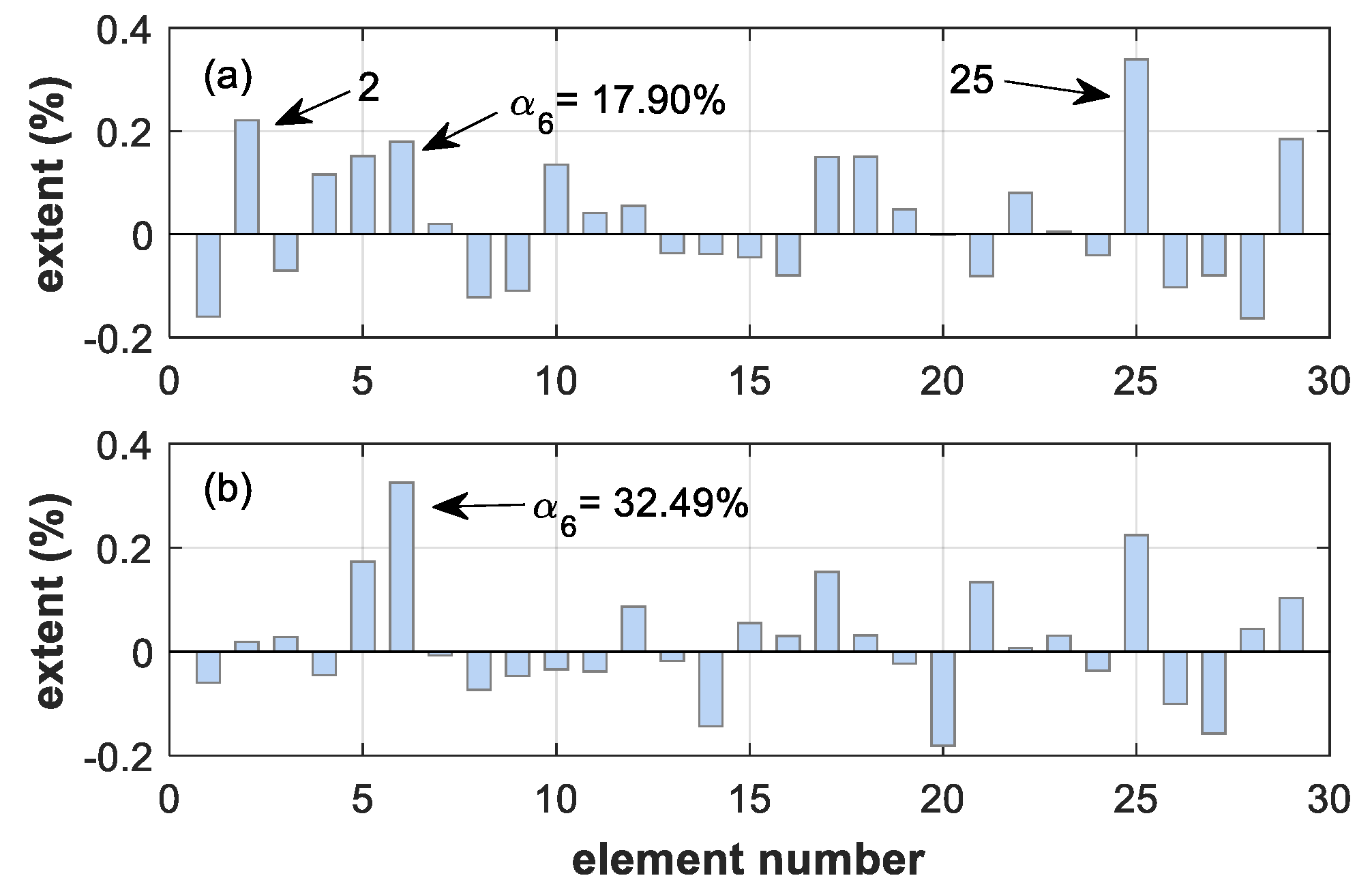
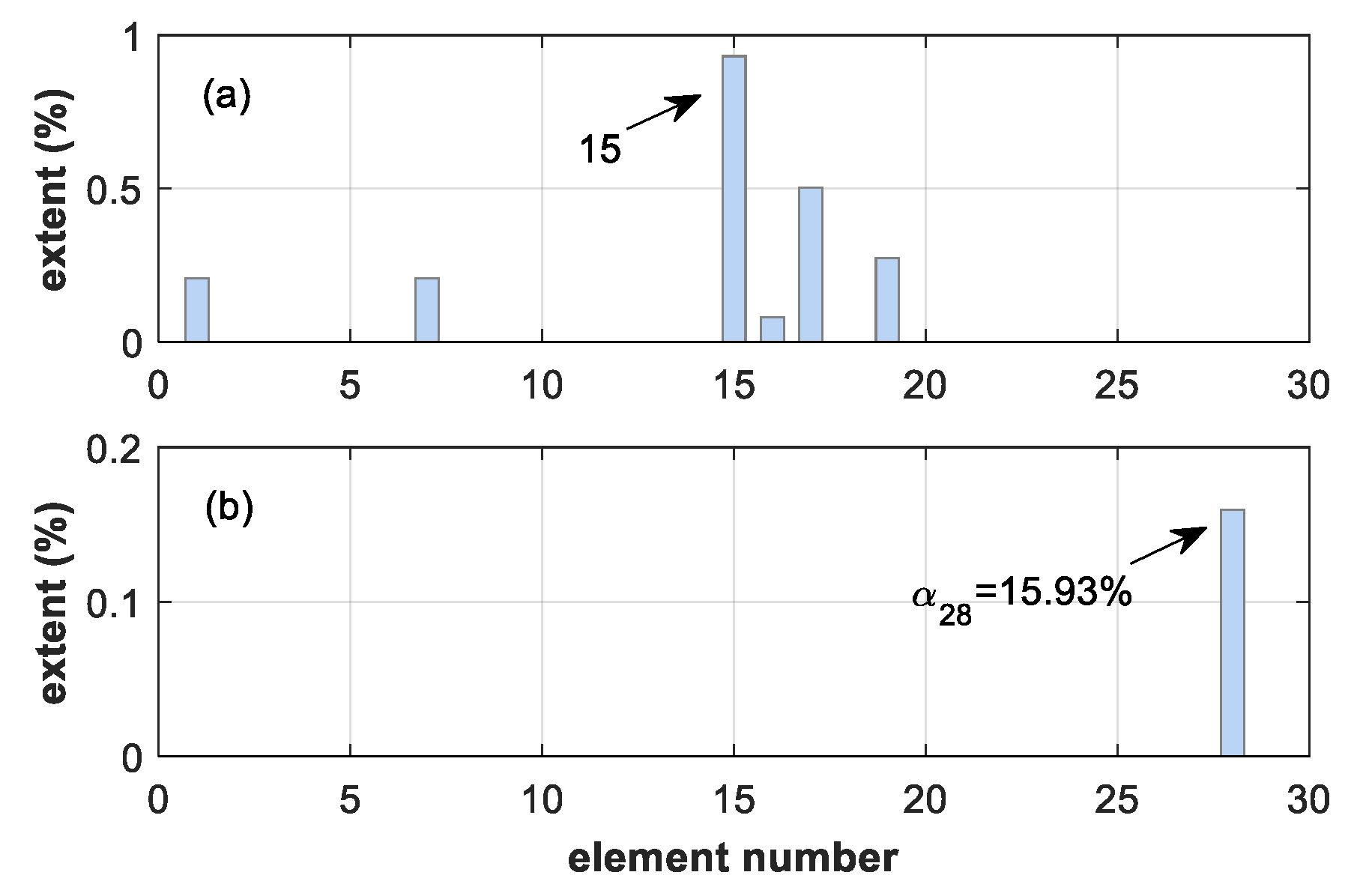
In this section, damage detection analysis is performed by considering different damage locations. It starts from damage case A ( α 6 = 30 % ) at a 3% level of noise. The least-squares method is firstly used to solve the CMSE system of linear equations. Figure 3 shows a comparison of the resulting location and extent of damage by using the classical CMSE and RCMSE methods.
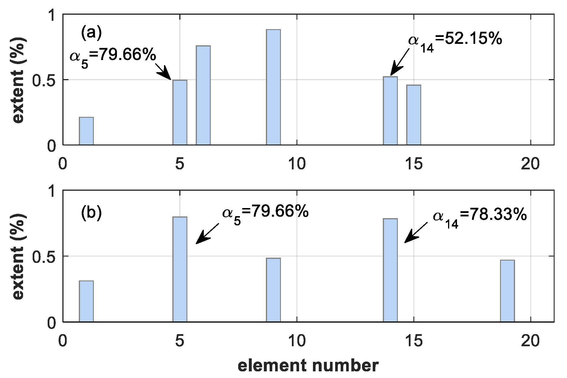
It is observed from Figure 3a that the localization indicator ambiguously locates the actually damaged element at a 3% level of noise, and both beam elements Nos. 2 and 25 seem to be candidates, as they are affected by the damage in the same way. Moreover, the estimated damage level of element No. 6 is far smaller than the expected value of 30%, indicating that the CMSE method cannot correctly detect stiffness reduction by using all 60 equations together.
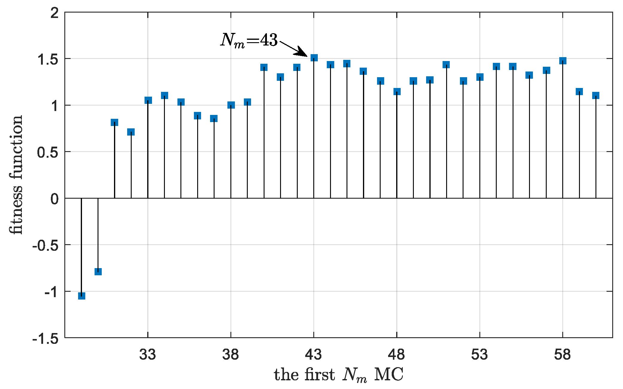
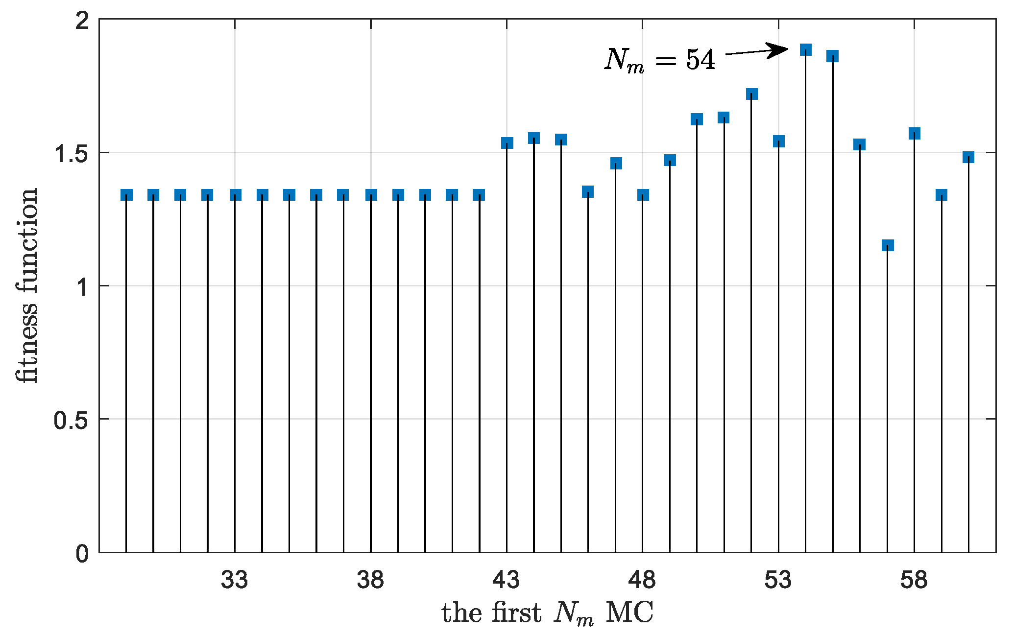
For the RCMSE method, a sensitivity analysis of the CMSE residual function with respect to damage is first performed to discriminate and eliminate redundant CMSE equations. Figure 4 shows the corresponding sensitivity indices of all 60 CMSE equations corresponding to 60 MCs. It is an expected result that the CMSE equations associated with the third mode of the damaged structure have larger sensitivity overall. The fitness function given in Figure 5 suggests that 43 equations are an optimum number for identifying the damage, so the CMSE system is reconstructed by eliminating 17 equations that correspond to the first 17 largest sensitivity indices, and damage identification analysis is performed again. It is shown in Figure 3b that the actual damage to element No. 6 is located accurately by the RCMSE method, whereas the estimated damage level is a little larger than the expected value, indicating that RCMSE outperforms the classical CMSE method both in damage localization and quantification.
Note that in Figure 5, only the fitness functions corresponding to 32 tested N m   ( N e N m N q ) are presented. This is because there are N e = 29 elements simulated for the 2-D truss structure, which also means at least 29 equations are required to ensure that the reduced CMSE system has a unique solution.
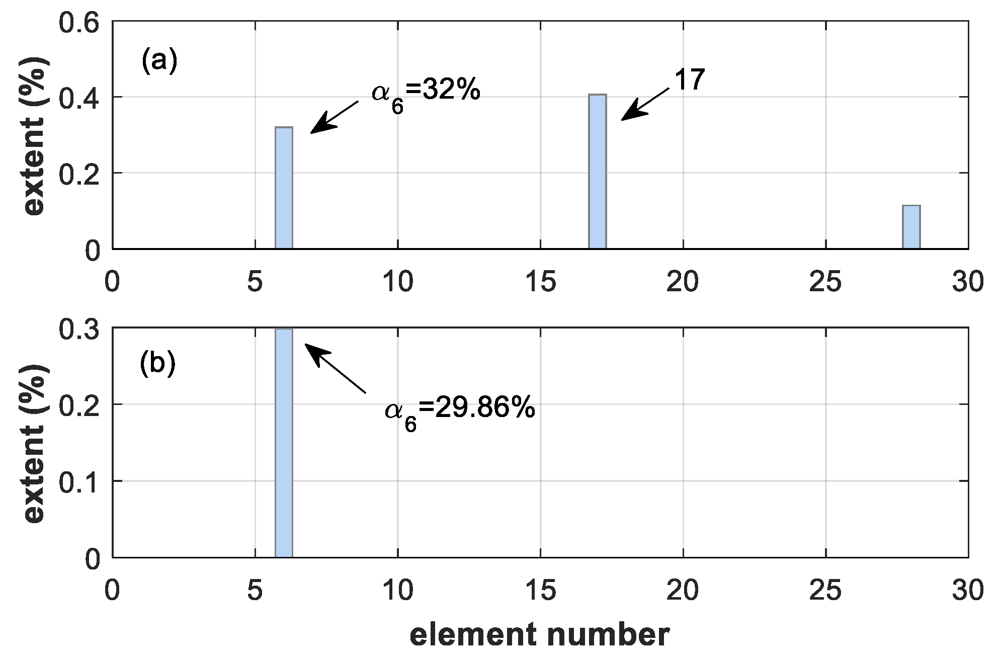
It is seen from Figure 3 that the damage identification results obtained by the least-squares method are not sparse, i.e., massive false-positive alarms of damage caused by noise contamination are produced, masking the actually damage-induced alarm. Here, an iterative Tikhonov solution can be tried to address this problem. Figure 6 shows a comparison between the identified results of the classical CMSE and RCMSE methods. By comparing Figure 3 and Figure 6, the obtained Tikhonov solutions are clearly sparse and the estimated extents of the actual damage are both closer to the expected value. This comparison illustrates that the ITR method can eliminate false-positive alarms of damage and is more suitable for detecting isolated damage to the structure. It is thus exclusively used to solve the CMSE system of linear equations hereafter.
It is also noted from Figure 6 that the RCMSE method remains more accurate than the classical CMSE method both in damage localization and quantification, even in terms of an iterative Tikhonov solution. This improvement strongly benefits from the elimination of 25 redundant equations according to the fitness function given by Figure 7. It can also be seen from Figure 7 that the fitness value obtained by using the corresponding first 35 equations is much larger than that obtained using all 60 equations, which illustrates that the predicted damage state of the structure agrees better with the real state when some redundant equations are eliminated.
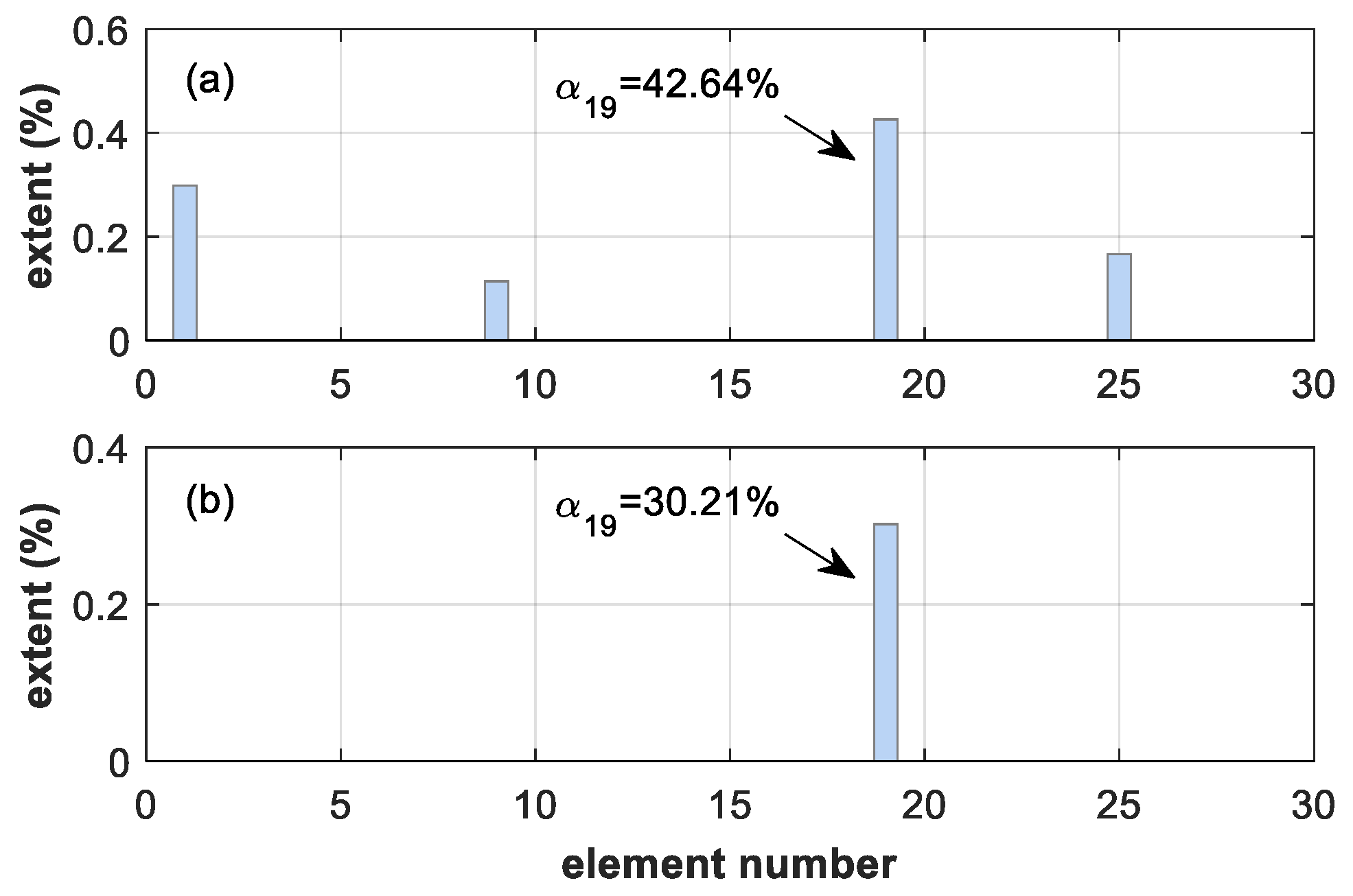
For damage case B, Figure 8 shows a comparison between the damage identification results of the CMSE and RCMSE methods. The top panel of Figure 8 illustrates that the damage of element No. 19 can be located by using all equations, but its extent is overestimated. In comparison, the RCMSE method, as shown in the bottom panel of Figure 8, exhibits enhancement of damage quantification.
It should be noted that in this case only 40 equations are used to predict the preset damage location and extent of damage (see Figure 9 and Figure 10), confirming that not all equations contribute to damage detection but complicate the CMSE system. Furthermore, by performing the analysis of CMSE equations’ sensitivity to damage, numerous redundant equations are eliminated, thereby simplifying the CMSE system.
For damage case C, the analysis of CMSE equations’ sensitivity to damage indicates that 54 equations are most appropriate for solving the preset location and extent of damage (see Figure 11 and Figure 12).
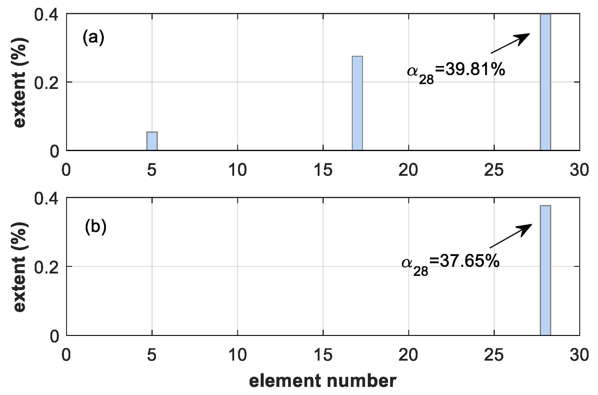
Following this, the CMSE method employing 60 equations and the RCMSE method employing 54 equations are used to identify the damage, respectively. Figure 13 shows that both methods can correctly locate the actual damage. However, two false-positive alarms of damage to elements Nos. 5 and 17 are produced when using the CMSE method. At the same time, both methods overestimate the preset extent of the damage. This reveals that the robustness of the CMSE method against noise is slightly improved by eliminating six redundant equations.
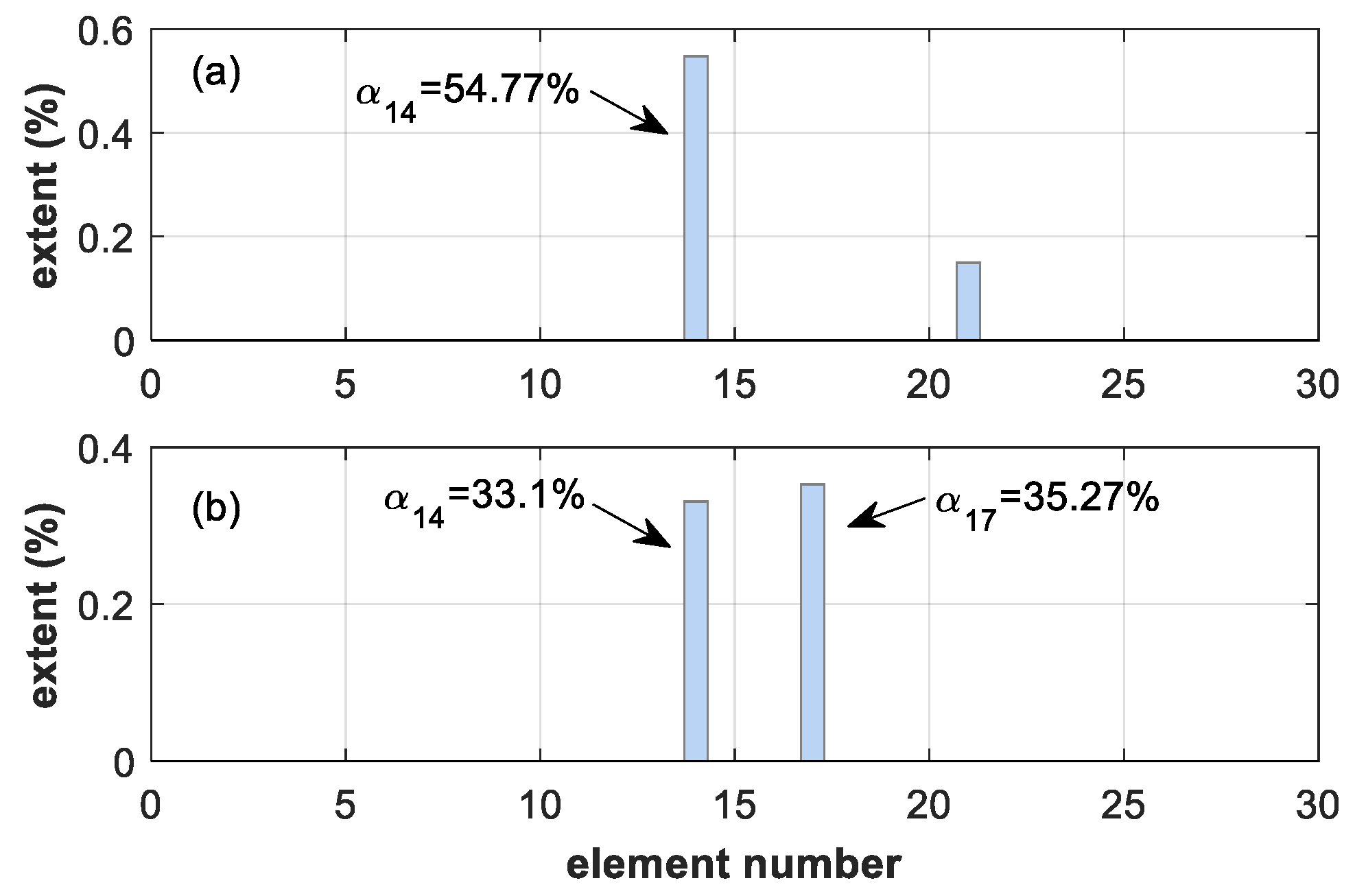
Damage case D is a double-damage case, in which elements Nos. 14 and 17 both exhibit a 30% stiffness loss. For this case, 45 equations are suggested for identifying damage according to the sensitivity analysis (see Table 2). The sensitivity index and fitness function are not shown here because of space limitations.
Figure 14 provides a comparison between the damage identification results of the CMSE and RCMSE methods. It is observed that the CMSE method omits the actually damaged element No. 17 and the extent of damage of element No. 14 is clearly overestimated. The RCMSE method demonstrates good damage localization and quantification performances, while it slightly overestimates the extent of the preset damage.
All results shown above demonstrate an improvement of damage identification by considering the sensitivity analysis scheme. It is worth noting that when the equation subsets are eliminated from the original CMSE system, the corresponding coefficient matrix of the reduced CMSE system, determining the accuracy of solution to some extent, is simplified. Hence, one would expect to explain this improvement from an ill-conditioned problem viewpoint. The condition number of the coefficient matrix C , defined as
κ = C * + · C *
measures how ill-conditioned a CMSE system is, where C * + is the Moore–Penrose inverse of C * because it is usually not a square matrix.
Table 2 shows the number of equations and the corresponding condition number of the original and reduced CMSE systems. It can be seen that in all simulated cases, the condition number is reduced as some redundant equations are eliminated. Taking damage case A as an example, the condition number is reduced from 126.36 to 95.92 as 25 equations are eliminated. This might confirm that a reasonable reduction of the dimension of the CMSE system yields a better-conditioned system and a better damage identification.
To further investigate the noise robustness of the proposed scheme, 1000 Monte Carlo simulations are performed by varying the level of noise from 0.5% to 5%. The damage identification probability [24] is used to measure the prediction accuracy, which is defined as
p d = n d n s × 100 %
where n s = 1000 is the total number of Monte Carlo simulations for a given level of noise and n d is the number of realizations in which the actual damage is detected.
Figure 15 shows the obtained damage identification probability of damage case A to damage case C, in which at least two findings are observable.
First, it is expected that the damage localization performance of the RCMSE method is better than that of the CMSE method at every level of noise, thereby confirming the effectiveness of eliminating redundant equations from the classical CMSE method.
Second, it is observed that for the CMSE method, the damage identification probability of DB element No. 28 and HB element No. 6 is always greater than that of HB element No. 19 in the examined range of noise level. When using a vibration-based method, the detectability of damage depends highly upon the modal parameter changes that the damage caused. It is observed by recalling Table 1 that the overall change in the first three natural frequencies due to the damage of element No. 19 is the smallest among these three damage cases, which may account for the difference in the damage localization performance of the CMSE method for different damage locations. However, for the RCMSE method, the damage identification probability of DB element No. 28 comes last. It is realized by comparing Figure 4, Figure 9 and Figure 11 that the MCs associated with the third mode of the damaged structure, on the whole, have larger sensitivity of the residual function to damage. In other words, the CMSE equations constructed by the third mode of the damaged structure are likely classified as redundant and eliminated from damage detection analysis. It can also be observed from Table 1 that the damage of element No. 28 mainly changes the third mode rather than the others. The discrepancy of the employed MCs may explain the different performances of these two methods.

4.3.2. Effects of Damage Level

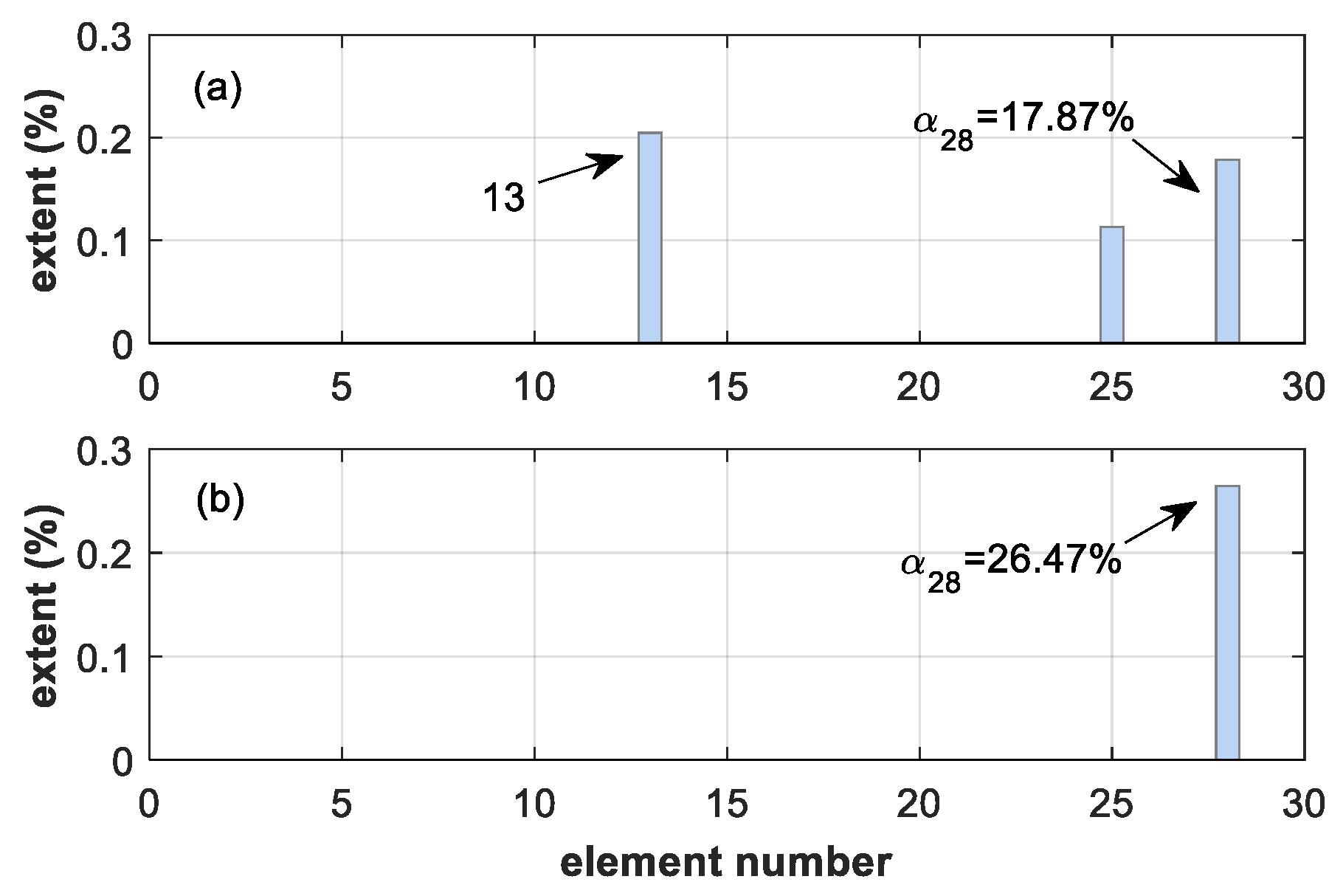
In this section, damage detection analysis is performed to consider how varying the damage level would affect the damage identification performance of the proposed scheme. The results of damage cases C ( α 28 = 30 % ), E ( α 28 = 20 % ), and F ( α 28 = 10 % ), are shown in Figure 13, Figure 16 and Figure 17, respectively.
Upon comparing the top panels of these three figures, as expected, the damage identification results of the classical CMSE method gradually worsen as the damage level decreases. Especially for damage case F, the actually damaged element No. 28 is classified as undamaged at a 3% level of noise. This demonstrates that the classical CMSE method has weak robustness against noise and its performance of the CMSE method is highly relevant to the damage level of the structure.
For the RCMSE method, it can be seen from the bottom panels of Figure 13, Figure 16 and Figure 17 that all damage cases are located, indicating the RCMSE method outperforms the classical CMSE method with regard to damage localization. Moreover, it can be seen that the RCMSE method always over- or under-estimates the extent of the damage. This is because, as mentioned earlier, the damage of element No. 28 mainly changes the third modal parameters of the structure; these parameters, however, contribute little to the damage detection analysis.
Table 3 shows the number of equations and the corresponding condition number of the original and reduced CMSE systems for damage cases E and F. It is also observed for each damage case that the condition number is reduced as some redundant equations are eliminated. This, again, confirms that reasonable reduction of the dimension of the CMSE system yields a better-conditioned system and better damage identification.
Then, 1000 Monte Carlo simulations are performed to obtain the identification probability of these three damage cases, and the results are displayed in Figure 18. Two findings are observable. First, by means of eliminating redundant equations and optimizing the construction of CMSE systems, the damage localization performance of the classical CMSE method is significantly improved. In addition, there is always a lower damage identification probability as the damage level decreases because severe damage always causes a larger change in the structural modal parameter. This trend also reveals that the CMSE and RCMSE methods are both sensitive to the damage level of the structure.

5. Experimental Validation

5.1. Description of the Beam Structure

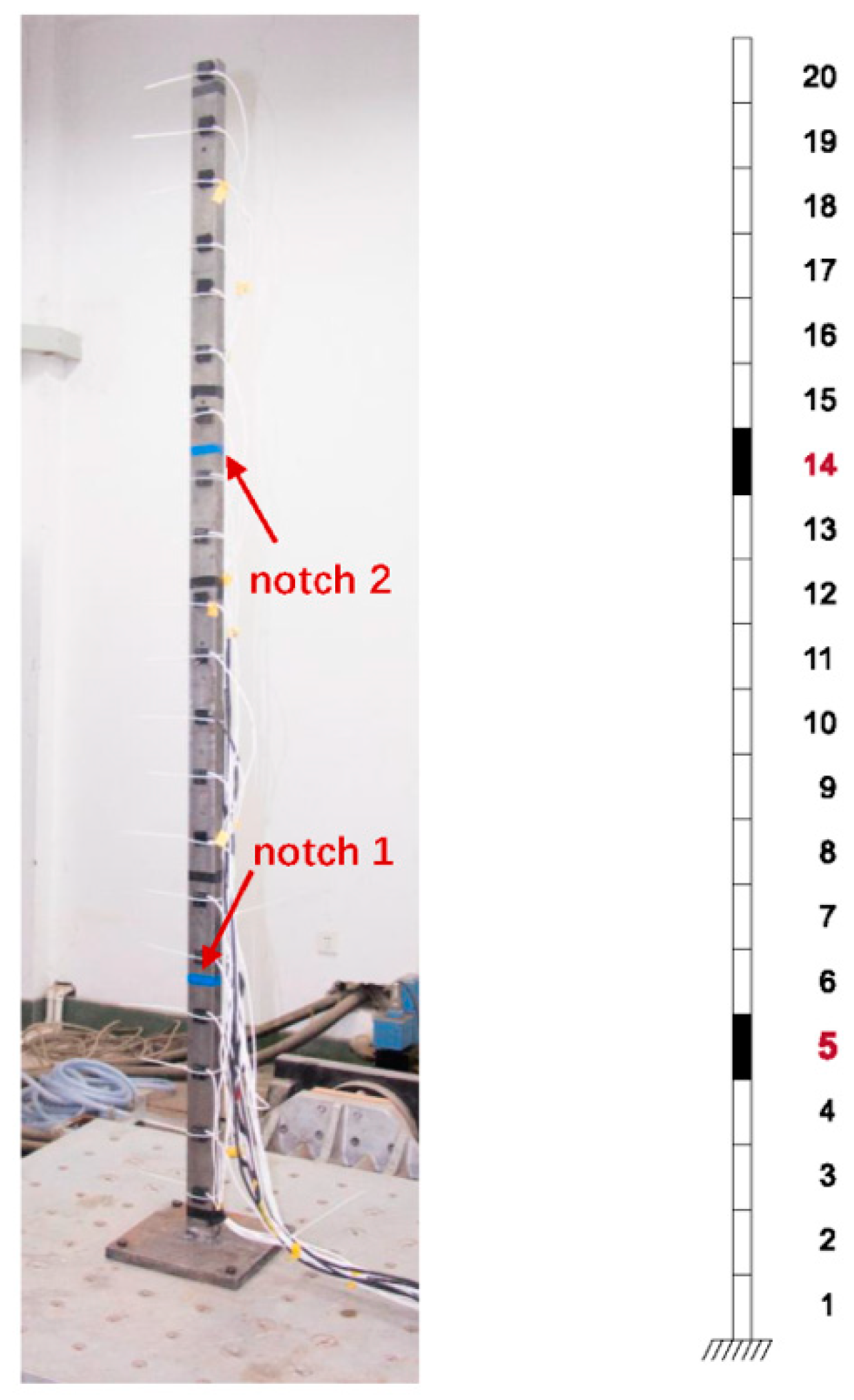
Experimental data from a cantilever beam structure are used to evaluate the effectiveness of the proposed damage identification scheme. The cantilever beam, as displayed in Figure 19, has a length, width, and thickness of 200, 5.0, and 2.8 cm, respectively, and is simulated by 20 equal Euler–Bernoulli beam elements.
Twenty accelerometers were vertically installed at every 10 cm on the beam to collect its acceleration time histories. A shock excitation on the beam was generated by means of an impulse hammer. To generate a maximum amplitude of the vibration signal, the impact location was selected at the free end of the beam. The excitation force was not measured. For output-only modal identification, the acceleration signal was processed by the eigensystem realization algorithm [35] to obtain the incomplete mode shapes, and Guyan’s method [36] was subsequently used for modal expansion.
The experiment started by measuring the dynamic responses of the undamaged beam, and a baseline FE model was constructed to represent the dynamic characteristics of the undamaged beam. Subsequently, two notches were generated by a saw cut on the beam in the width direction. Again, the dynamic responses of the damaged beam were measured for modal identification and damage detection. Three damage cases including two single- and one double-damage cases were considered by producing two notches. As shown in Figure 19, the location of the first notch was 44.2 cm away from the clamped end of the beam, approximately at the middle of element No. 5, and the second notch was located approximately at the middle of element No. 14. Two extents of damage are considered, including the notch depths of about 1/4 and 1/2 of the beam thickness. The length of the notch along the beam axis was about 1 mm. In the experiment, the first three modes of the beam were always identified from the measurement data, i.e., N j = 3 . The simulated damage cases and the measured natural frequencies are listed in Table 4 for clarity.
The essential geometric and material properties of the baseline FE model are as follows. The linear mass density is 7920 kg/m3 by considering the mass of beam, sensors, and wires; and the Young’s modulus of the elements at the non-clamped position is uniformly 1.91 × 10¹¹ N/m2, whereas that of the element at the clamped edge is reduced to 1.80 × 10¹¹ N/m2 to consider the possibly imperfect connection.
To examine the accuracy of the baseline FE model, an eigenvalue analysis was performed to obtain its modal characteristics, i.e., the analytical modal parameters. The measured and analytical natural frequencies and mode shape correlations represented by modal assurance criterions (MACs) are summarized in Table 5 for clarity. It is evident that the analytical modal parameters match the corresponding measured values very well, thereby confirming the accuracy of the model updating process.

5.2. Results and Discussions

In this experiment, the first 15 modes of the undamaged beam calculated from the updated baseline FE model as well as the first 3 modes of the damaged beam identified from the measured data are used for damage identification. That is to say, a total of 45 CMSE equations can be formed. Therefore, for the classical CMSE method, 45 equations are always used to identify the damage, whereas for the RCMSE method, an analysis of the residual function’s sensitivity to damage is performed first to discriminate redundant equations.
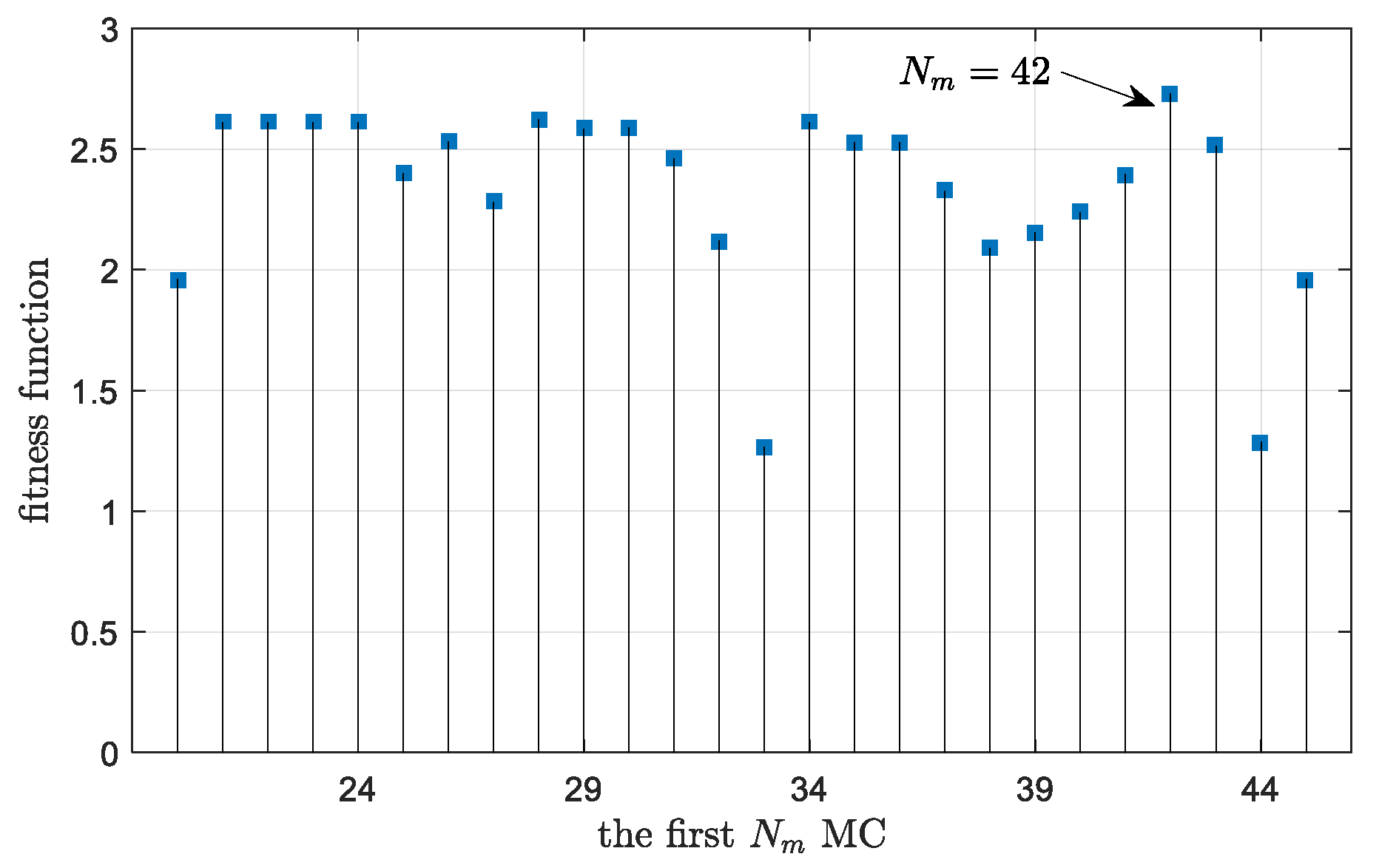
For damage case I (1/4-thickness notch), Figure 20 and Figure 21 give the 42 equations that are most appropriate to solve the actual location and extent of the damage. Then, these equations are selected to construct the CMSE system.
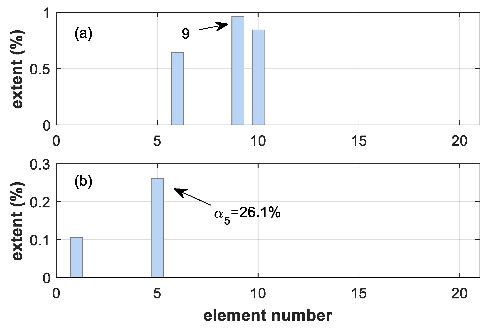
Figure 22 shows a comparison of the resulting location and extent of damage by using the classical CMSE and the RCMSE methods. It is evident that the damage of element No. 5 can be located by the RCMSE method but cannot be located by the CMSE method, indicating an enhancement of damage identification by eliminating three redundant equations.
It is worth mentioning that the performance of the CMSE and RCMSE methods with regard to damage severity estimation is not discussed here. This is because the actual stiffness reduction of the beam is unknown.
For damage case II (1/2-thickness notch), 43 equations are used to identify damage for the RCMSE method. One can observe from Figure 23 that damage at element No. 5 also can be located clearly by the RCMSE method. However, for the classical CMSE method, although the actually damaged element can be identified, a false-alarm of damage at element No. 15 is also produced. The difference between the results, again, illustrates the effectiveness of the elimination of redundant equations.
Furthermore, by comparing Figure 22b and Figure 23b, it can be seen that RCMSE also produces a false-positive damage at element No. 1 for damage case I, hinting that smaller damage always results in a smaller change in the structural modal parameter (see Table 4) and leads to lower damage detectability.
For damage case III (1/2-thickness notches), 23 equations are used to identify damage for the RCMSE method. Figure 24 shows that both methods cannot yield a sparse solution. In other words, both methods produce several false-positives of damage except for the correct indications of damage at elements Nos. 5 and 14. This illustrates that double-damage is difficult to identify for both methods. However, it is also shown that the estimated extents of damage at the actually damaged locations by the RCMSE method are greater than others. In other words, the actually damaged elements are not masked by false-positives. In addition, the estimated extents of these two damaged elements, i.e., for both 1/2-thickness notches, by the RCMSE method are almost the same, implicating an improvement in damage identification performance as compared to the CMSE method.

6. Conclusions

This paper presented a CMSE-based damage identification scheme. An analysis of the defined residual function’s sensitivity to damage was performed to measure how the actual damage level vector satisfied each CMSE equation. A sensitivity index was formulated to discriminate and eliminate the redundant equations that do not contribute to damage detection but complicate the system. The numerical and experiment robustness of the proposed damage identification scheme against measurement noise was investigated. Two main aspects were emphasized by the results.
First, the damage identification performance of the classical CMSE method was clearly improved by eliminating redundant equations from the original CMSE system, confirming the validity of the sensitivity analysis process. The improvement of damage identification might inherently benefit from an improvement of the originally ill-conditioned problem by a reasonable reduction of the dimension of the CMSE system.
Second, for the proposed CMSE-based damage identification scheme, the detectability of damage depended highly upon the modal parameter changes that the damage caused. For different locations of damage even with the same damage level, the resulting modal parameter change in different modes varied, and the employed modes were also different. This is the reason for the discrepancy of the damage localization performance for different damage locations. Besides, the damage identification probability gradually decreased as the damage level decreased. The phenomenon is due to the fact that smaller damage always results in a smaller change in structural modal parameters and leads to lower damage detectability.
Overall, this study provides a contribution towards a clear and simple guideline for eliminating redundant equations in order to enhance the robustness of the CMSE system, which is solved by the ITR method to obtain spare solutions. Since a broad range of regression techniques [37,38] that can solve the CMSE system are now available, it is extremely necessary to compare the performance of the ITR method and these state-of-art techniques.

Author Contributions

Funding acquisition, S.W. and Y.L.; Investigation, M.X., J.G. and Y.L.; Methodology, M.X. and S.W.; Software, M.X., J.G. and S.W.; Supervision, S.W.; Validation, S.W. and Y.L.; Experiment, S.W.; Writing—Original draft, M.X.; Writing—Review and Editing, M.X., Y.L. and S.W. All authors have read and agreed to the published version of the manuscript.

Funding

This work was supported by the National Science Fund for Distinguished Young Scholars (51625902), the National Key Research and Development Program of China (2019YFC0312404), the Major Scientific and Technological Innovation Project of Shandong Province (2019JZZY010820), the National Natural Science Foundation of China (51809134), the Natural Science Foundation of Shandong Province (ZR2017MEE007), and the Taishan Scholars Program of Shandong Province (TS201511016).

Conflicts of Interest

The authors declare no potential conflicts of interest with respect to the research, authorship, and/or publication of this article.

References

  1. Flynn, E.B.; Todd, M.D. A Bayesian approach to optimal sensor placement for structural health monitoring with application to active sensing. Mech. Syst. Signal Process. 2010, 24, 891–903. [Google Scholar] [CrossRef]
  2. Pérez, J.E.R.; Rodríguez, R.; Vázquez-Hernández, A.O. Damage detection in offshore jacket platforms with limited modal information using the damage submatrices method. Mar. Struct. 2017, 55, 78–103. [Google Scholar] [CrossRef]
  3. Oliveira, G.; Magalhães, F.; Cunha, Á.; Caetano, E. Vibration-based damage detection in a wind turbine using 1 year of data. Struct. Control Health Monit. 2018, 25, e2238. [Google Scholar] [CrossRef]
  4. Soman, R.; Mieloszyk, M.; Ostachowicz, W. A two-step damage assessment method based on frequency spectrum change in a scaled wind turbine tripod with strain rosettes. Mar. Struct. 2018, 61, 419–433. [Google Scholar] [CrossRef]
  5. Chaabane, M.; Mansouri, M.; Ben Hamida, A.; Nounou, H.; Nounou, M. Multivariate statistical process control-based hypothesis testing for damage detection in structural health monitoring systems. Struct. Control Health Monit. 2019, 26, e2287. [Google Scholar] [CrossRef] [Green Version]
  6. Ding, Z.H.; Li, J.; Hao, H. Structural damage identification using improved Jaya algorithm based on sparse regularization and Bayesian inference. Mech. Syst. Signal Process. 2019, 132, 211–231. [Google Scholar] [CrossRef]
  7. Wang, S.Q.; Wang, H.Y.; Xu, M.Q.; Guo, J. Identifying the presence of structural damage: A statistical hypothesis testing approach combined with residual strain energy. Mech. Syst. Signal Process. 2020, 140, 106655. [Google Scholar] [CrossRef]
  8. Shi, Z.Y.; Law, S.S.; Zhang, L.M. Structural damage localization from modal strain energy change. J. Eng. Mech. 2000, 218, 1216–1223. [Google Scholar] [CrossRef]
  9. Zhu, H.P.; Xu, Y.L. Damage detection of mono-coupled periodic structures based on sensitivity analysis of modal parameters. J. Sound Vib. 2005, 285, 365–390. [Google Scholar] [CrossRef]
  10. Hu, S.L.J.; Wang, S.Q.; Li, H.J. Cross-Modal Strain Energy Method for Estimating Damage Severity. J. Eng. Mech. 2006, 132, 429–437. [Google Scholar]
  11. Zhan, J.W.; Xia, H.; Chen, S.Y.; Roeck, G.D. Structural damage identification for railway bridges based on train-induced bridge responses and sensitivity analysis. J. Sound Vib. 2011, 330, 757–770. [Google Scholar] [CrossRef]
  12. Zheng, Z.D.; Lu, Z.R.; Chen, W.H.; Liu, J.K. Structural damage identification based on power spectral density sensitivity analysis of dynamic responses. Comput. Struct. 2015, 146, 176–184. [Google Scholar] [CrossRef]
  13. Golub, G.; Hansen, P.; O’Leary, D. Tikhonov regularization and total least squares. J. Matrix Anal. Appl. 1999, 21, 185–194. [Google Scholar] [CrossRef] [Green Version]
  14. Calvetti, D.; Morigi, S.; Reichel, L.; Sgallari, F. Tikhonov regularization and the L-curve for large discrete ill-posed problems. J. Comput. Appl. Math. 2000, 123, 423–446. [Google Scholar] [CrossRef] [Green Version]
  15. Hansen, P.C. Analysis of Discrete Ill-Posed Problems by Means of the L-Curve. SIAM Rev. 1992, 34, 561–580. [Google Scholar] [CrossRef]
  16. Zhang, C.D.; Xu, Y.L. Comparative studies on damage identification with Tikhonov regularization and sparse regularization. Struct. Control Health Monit. 2016, 23, 560–579. [Google Scholar] [CrossRef]
  17. Entezami, A.; Shariatmadar, H.; Sarmadi, H. Structural damage detection by a new iterative regularization method and an improved sensitivity function. J. Sound Vib. 2017, 399, 285–307. [Google Scholar] [CrossRef]
  18. Fan, X.; Li, J.; Hao, H.; Ma, S. Identification of Minor Structural Damage Based on Electromechanical Impedance Sensitivity and Sparse Regularization. J. Aerosp. Eng. 2018, 31, 04018061. [Google Scholar] [CrossRef]
  19. Weber, B.; Paultre, P.; Proulx, J. Structural damage detection using nonlinear parameter identification with Tikhonov regularization. Struct. Control Health Monit. 2007, 14, 406–427. [Google Scholar] [CrossRef]
  20. Rezaiee-Pajand, M.; Entezami, A.; Sarmadi, H. A sensitivity-based finite element model updating based on unconstrained optimization problem and regularized solution methods. Struct. Control Health Monit. 2020, 27, e2481. [Google Scholar] [CrossRef]
  21. Yan, G.; Sun, H.; Büyüköztürk, O. Impact load identification for composite structures using Bayesian regularization and unscented Kalman filter. Struct. Control Health Monit. 2017, 24, e1910. [Google Scholar] [CrossRef]
  22. Björck, Å. A bidiagonalization algorithm for solving large and sparse ill-posed systems of linear equations. BIT Numer. Math. 1988, 28, 659–670. [Google Scholar] [CrossRef]
  23. Golub, G.H.; Heath, M.; Wahba, G. Generalized Cross-Validation as a Method for Choosing a Good Ridge Parameter. Technometrics 1979, 21, 215–223. [Google Scholar] [CrossRef]
  24. Wang, S.Q.; Xu, M.Q.; Xia, Z.P.; Li, Y.C. A novel Tikhonov regularization-based iterative method for structural damage identification of offshore platforms. J. Mar. Sci. Technol. 2019, 24, 575–592. [Google Scholar] [CrossRef]
  25. Carden, E.P.; Fanning, P. Vibration Based Condition Monitoring: A Review. Struct. Health Monit. 2004, 3, 355–377. [Google Scholar] [CrossRef]
  26. Yan, Y.J.; Cheng, L.; Wu, Z.Y.; Yam, L.H. Development in Vibration-Based Structural Damage Detection Technique. Mech. Syst. Signal Process. 2007, 21, 2198–2211. [Google Scholar] [CrossRef]
  27. Fan, W.; Qiao, P.Z. Vibration-based Damage Identification Methods: A Review and Comparative Study. Struct. Health Monit. 2011, 10, 83–111. [Google Scholar] [CrossRef]
  28. Dessi, D.; Camerlengo, G. Damage identification techniques via modal curvature analysis: Overview and comparison. Mech. Syst. Signal Process. 2015, 52, 181–205. [Google Scholar] [CrossRef]
  29. Wang, S.Q.; Xu, M.Q. Modal Strain Energy-based Structural Damage Identification: A Review and Comparative Study. Struct. Eng. Int. 2019, 29, 234–248. [Google Scholar] [CrossRef]
  30. Xu, M.Q.; Wang, S.Q.; Jiang, Y.F. Iterative two-stage approach for identifying structural damage by combining the modal strain energy decomposition method with the multiobjective particle swarm optimization algorithm. Struct. Control Health Monit. 2019, 26, e2301. [Google Scholar] [CrossRef]
  31. Wang, S.Q.; Li, H.J.; Hu, S.L.J. Cross Modal Strain Energy Method for Damage Localization and Severity Estimation. In Proceedings of the ASME 2007 26th International Conference on Offshore Mechanics and Arctic Engineering, San Diego, CA, USA, 10–15 June 2007; pp. 245–249. [Google Scholar]
  32. Yan, W.J.; Ren, W.X. A direct algebraic method to calculate the sensitivity of element modal strain energy. Int. J. Numer. Methods Biomed. Eng. 2011, 27, 694–710. [Google Scholar] [CrossRef]
  33. Lee, I.W.; Jung, G.H. An efficient algebraic method for the computation of natural frequency and mode shape sensitivities—Part I. Distinct natural frequencies. Comput. Struct. 1997, 62, 429–435. [Google Scholar] [CrossRef]
  34. Messina, A.; Williams, E.J.; Contursi, T. Structural damage detection by a sensitivity and statistical-based method. J. Sound Vib. 1998, 216, 791–808. [Google Scholar] [CrossRef]
  35. Juang, J.N.; Pappa, R.S. An eigensystem realization algorithm for modal parameter identification and model reduction. J. Guid. Control Dyn. 1985, 8, 620–627. [Google Scholar] [CrossRef]
  36. Guyan, R.J. Reduction of stiffness and mass matrices. AIAA J. 1965, 3, 380. [Google Scholar] [CrossRef]
  37. Bertsimas, D.; King, A.; Mazumder, R. Best Subset Selection via a Modern Optimization Lens. Mathematics 2016, 44, 813–852. [Google Scholar] [CrossRef] [Green Version]
  38. Hastie, T.; Tibshirani, R.; Tibshirani, R.J. Extended Comparisons of Best Subset Selection, Forward Stepwise Selection, and the Lasso. arXiv 2017, arXiv:1707.08692. [Google Scholar]
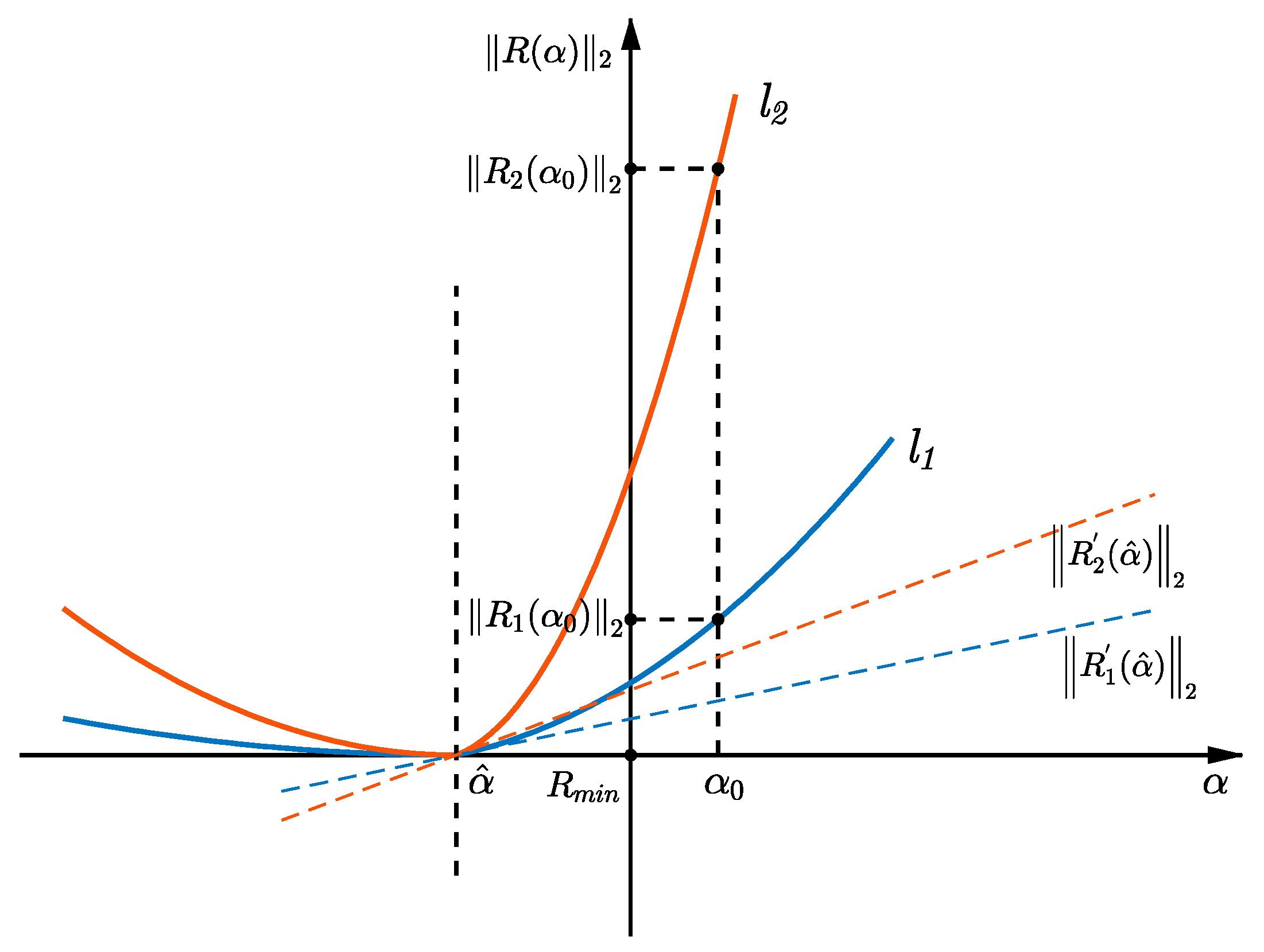
Figure 1. A comparison of two residual sub-functions with different residual-damage sensitivity.
Applsci 10 02826 g001
Figure 2. Sketch of the truss structure.
Applsci 10 02826 g002
Figure 3. The damage identification results of damage case A at a 3% level of noise, with the least-squares solution: (a) CMSE method; (b) RCMSE method.
Applsci 10 02826 g003
Figure 4. The sensitivity index of damage case A versus MCs N i = 20 and N j = 3 , at a 3% level of noise.
Applsci 10 02826 g004
Figure 5. Fitness function of damage case A at a 3% level of noise for the least-squares method.
Applsci 10 02826 g005
Figure 6. Damage identification results of damage case A at a 3% level of noise, with an iterative Tikhonov solution: (a) CMSE method; (b) RCMSE method.
Applsci 10 02826 g006
Figure 7. Fitness function of damage case A at a 3% level of noise, for the ITR method.
Applsci 10 02826 g007
Figure 8. Damage identification results of damage case B at a 3% level of noise, with an iterative Tikhonov solution: (a) CMSE method; (b) RCMSE method.
Applsci 10 02826 g008
Figure 9. Sensitivity index of damage case B versus MCs N i = 20 and N j = 3 , at a 3% level of noise.
Applsci 10 02826 g009
Figure 10. Fitness function of damage case B at a 3% level of noise, for the ITR method.
Applsci 10 02826 g010
Figure 11. Sensitivity index of damage case C versus MCs N i = 20 and N j = 3 , at a 3% level of noise.
Applsci 10 02826 g011
Figure 12. Fitness function of damage case C at a 3% level of noise, for the ITR method.
Applsci 10 02826 g012
Figure 13. Damage identification results of damage case C at a 3% level of noise, with an iterative Tikhonov solution: (a) CMSE method; (b) RCMSE method.
Applsci 10 02826 g013
Figure 14. Damage identification results of damage case D at a 3% level of noise, with an iterative Tikhonov solution: (a) CMSE method; (b) RCMSE method.
Applsci 10 02826 g014
Figure 15. The identification probability of damage cases A to C against the level of noise.
Applsci 10 02826 g015
Figure 16. Damage identification results of damage case E at a 3% level of noise, with an iterative Tikhonov solution: (a) CMSE method; (b) RCMSE method.
Applsci 10 02826 g016
Figure 17. Damage identification results of damage case F at a 3% level of noise, with an iterative Tikhonov solution: (a) CMSE method; (b) RCMSE method.
Applsci 10 02826 g017
Figure 18. Identification probability of damage cases C, E, and F against the level of noise.
Applsci 10 02826 g018
Figure 19. Beam structure used in the experiment, physical (left) and finite element (right) models.
Applsci 10 02826 g019
Figure 20. Sensitivity index of damage case I versus MCs N i = 15 and N j = 3 .
Applsci 10 02826 g020
Figure 21. Fitness function of damage case I, for the ITR method.
Applsci 10 02826 g021
Figure 22. Damage identification results of damage case I, with an iterative Tikhonov solution: (a) CMSE method; (b) RCMSE method.
Applsci 10 02826 g022
Figure 23. Damage identification results of damage case II, with an iterative Tikhonov solution: (a) CMSE method; (b) RCMSE method.
Applsci 10 02826 g023
Figure 24. Damage identification results of damage case III, with an iterative Tikhonov solution: (a) CMSE method; (b) RCMSE method.
Applsci 10 02826 g024
Table 1. The simulated damage cases of the truss structure.
Damage CaseLocationExtentNatural Frequencies (Hz)
1st2nd3rd
BaselineN/AN/A13.87822.25723.832
A630%13.84522.07423.634
B1930%13.87721.99623.740
C2830%13.70122.16623.601
D14, 1730%, 30%13.83721.94623.761
E2820%13.77422.20223.686
F2810%13.83222.23223.763
Table 2. The number of equations ( N m ) and the corresponding condition number ( κ ) of the original and reduced CMSE systems for damage cases A to D.
Damage CaseOriginal SystemReduced System
N m κ N m κ
A60126.363595.92
B60126.794028.23
C60128.455422.31
D60123.864555.15
Table 3. The number of equations ( N m ) and the corresponding condition number ( κ ) of the original and reduced CMSE systems for damage cases E and F.
Damage CaseOriginal SystemReduced System
N m κ N m κ
E60126.305636.61
F60124.034025.71
Table 4. Simulated damage cases and measured natural frequencies in the experiment.
CaseLocationExtentNatural Frequencies (Hz)
1st2nd3rd
UndamagedN/AN/A5.52434.71197.200
I51/4 thickness5.47334.76896.874
II51/2 thickness5.29934.75595.089
III5 and 141/2 and 1/2 thickness5.28933.83791.485
Table 5. Measured and analytical natural frequencies and MACs of the undamaged beam.
Data TypeNatural Frequencies (Hz)MACs
1st2nd3rd1st2nd3rd
Measured5.52434.71197.2000.9990.9970.998
Analytical5.52334.64497.079