Abstract
To study the variations in modal properties of a reinforced concrete (RC) slab (such as natural frequencies, mode shapes and damping ratios) under the influence of ambient temperature, a laboratory RC slab is monitored for over a year, the simple linear regression (LR) and autoregressive with exogenous input (ARX) models between temperature and frequencies are established and validated, and a damage identification based on particle swarm optimization (PSO) is utilized to detect the assumed damage considering temperature effects. Firstly, the vibration testing is performed for one year and the variations of natural frequencies, mode shapes and damping ratios under different ambient temperatures are analyzed. The obtained results show that the change of ambient temperature causes a major change of natural frequencies, which, on the contrary, has little effect on damping ratios and modal shapes. Secondly, based on a theoretical derivation analysis of natural frequency, the models are determined from experimental data on the healthy structure, and the functional relationship between temperature and elastic modulus is obtained. Based on the monitoring data, the LR model and ARX model between structural elastic modulus and ambient temperature are acquired, which can be used as the baseline of future damage identification. Finally, the established ARX model is validated based on a PSO algorithm and new data from the assumed 5% uniform damage and 10% uniform damage are compared with the models. If the eigenfrequency exceeds the certain confidence interval of the ARX model, there is probably another cause that drives the eigenfrequency variations, such as structural damage. Based on the constructed ARX model, the assumed damage is identified accurately.
1. Introduction
Actual civil structures are susceptible to the influence of varying environmental factors and operational conditions such as humidity, wind and moving vehicles, however the most important factor has proven to be temperature [1,2,3]. In recent years, structural health monitoring under environmental variations has become a popular research topic in the field of civil engineering [4,5,6]. Moaveni and Behmanesh [7] investigated the effects of changing ambient temperatures on finite element (FE) model updating of the Dowling Hall Footbridge. Moorty and Roeder [8] studied temperature-dependent bridge movements and stress development in bridges. Liang et al. [9] proposed a new data normalization technique based on the improved restoring force model (IRFM) to distinguish the effect of damage from those caused by environmental and operational variations. Grosso and Lanata [10] conducted a static continuous monitoring experiment to assess the validity of some damage detection algorithms. Li et al. [11] proposed a damage identification approach in bridge structures under moving vehicular loads without knowledge of the vehicle properties and the time-histories of moving interaction forces. Yarnold and Moon [12] utilized the relationship between temperature changes and the resulting strains and displacements of the structure to create a unique numerical and graphical baseline within an structural health monitoring (SHM) framework and found the temperature-based approach was more sensitive for the scenarios examined. Chang et al. [13] investigated the feasibility of the pseudo-static damage identification method derived from a bridge–vehicle interaction system through a moving vehicle laboratory experiment.
For structural damage identification, damage is generally identified through the dynamic characteristics test of the structures by analyzing the change of structural modal parameters, such as natural frequencies, mode shapes, and damping ratios. Doebling et al. [14,15] provided an overview of methods to detect, locate, and characterize damage in structural and mechanical systems by examining changes in measured vibration response. Hao and Xia [16] proposed a genetic algorithm (GA) with real number encoding to identify the structural damage by minimizing the objective function, which directly compares the changes in the measurements before and after damage occurs. Deraemaeker and Preumont [17] introduced a novel approach for vibration-based damage detection, which is based on the use of a large network of sensors’ frequency response function (FRF). Boonlong [18] performed a vibration-based damage detection of a beam based on a cooperative co evolutionary GA. However, dynamic characteristics such as natural frequencies, mode shapes and damping ratios are inherently susceptible not only to structural damage but also environmental variations and operational conditions, and it is the variation of temperature that induces major fluctuation of structural dynamic parameters [19]. Among the many factors that affect the modal frequency of the bridge structure, the change of the modal frequency caused by temperature may be larger than that caused by structural damage, and the change caused by small damage to the structure is even submerged or masked. Therefore, it is of great significance to study the effect of temperature on modal properties. Alampalli [20] took an experiment for one small steel truss bridge and found that the influence of temperature on frequency exceeds the influence of simulated fault on frequency. Peeters et al. [21] carried out a 10-month dynamic test on Z24 Bridge and found that the fluctuation range of the 1st to 4th natural frequencies of the bridge was 14%, 18%, 16% and 17%, respectively. Zhao and DeWolf [22] monitored a steel plate girder bridge for 2 years and it is shown that the natural frequency change at the lowest temperature (−15.6 °C) compared with the reference temperature (12.8 °C) could be up to 15.4%. Xu and Wu [23] found that changes in dynamic characteristics of the bridge due to damage in girders or cables may be smaller than changes in dynamic characteristics due to variations in temperature. Martins et al. [24] investigated the variation of wind, temperature and acceleration of the Braga Stadium suspension roof during a period of 8 months and analyzed the influence of wind and temperature on the variation of modal parameters.
To distinguish the modal parameter change caused by structural damage and temperature change, many methods are adopted to identify the structural damage considering temperature variations. Huang et al. [25] proposed a non-destructive global damage identification method based on a genetic algorithm (GA) to identify the damage location and severity of the structure under the influence of temperature variation and noise, which is verified by a number of damage scenarios using a three-span continuous beam. It shows good robustness under random noise levels with a lab steel grid experiment. Jin et al. [26] developed an extended Kalman filter-based artificial neural network (EKFNN) method to eliminate the temperature effects and detect damage for structures equipped with long-term monitoring systems, and the correlations between natural frequencies and temperature are analyzed to select proper input variables for the neural network model. Jiao et al. [27] proposed a fuzzy neural network-based damage assessment method, in which uniform load surface curvature is used as damage indicator. Under the assumption that the elasticity modulus of concrete is temperature dependent, the algorithm can distinguish the damage from the temperature effect.
The relationship between frequency and temperature variations are constructed to study the influence of temperature on frequency. The purpose is to quantify the relationship between temperature and natural eigenfrequency. Ni et al. [28] adopted support vector machine (SVM) to analyze the monitoring data and quantify the influence of temperature on modal frequency, the results obtained by the SVM models are compared with those produced by a multivariate linear regression model, and it is shown that the SVM models exhibit good capabilities for mapping between the temperature and modal frequencies. Farrar et al. [29] monitored the natural variability of the frequencies and mode shapes of the Alamosa Canyon Bridge that result from changes in time of day considering the amount of traffic and environmental conditions. Peeters and Roeck [21] monitored the Z24 Bridge and proposed a black-box model to describe the variations of eigenfrequencies as a function of temperature, and new data are compared with the models to discriminate the reason that induced the changes of eigenfrequency. Sohn et al. [30] proposed a linear adaptive model to discriminate the changes of modal parameters due to temperature changes from those caused by structural damage or other environmental effects. Xia et al. [31] monitored the influence of temperature and humidity on the vibration characteristics of the structure, and linear regression models between modal properties and environmental factors were built. Liu et al. [32] established a multiple linear regression model (MLRM) to describe the relationship between modal frequency and non-uniform temperature distribution to raise the accuracy of quantified temperature and frequency. Zhou et al. [33] obtained the correlation between temperature and frequency by comparing the test data of a simply supported beam under the effect of temperature.
Few researches focus on the damage identification based on the established relationship model, such as the linear regressive model and the autoregressive with exogenous (ARX) model. When the damage causes the nonlinear response of the structure, it is expected that the residual damage will increase. Therefore, the standard deviation of residual damage is predicted as the damage characteristic quantity by using ARX model. The results show that this method can detect the damage. In this paper, continuous vibration testing is carried out for one year. Based on the acquired vibration testing, the simple LR model and ARX model between the first four eigenfrequencies and temperatures are established. By comparing the root mean squared error (RMSE) between the simple LR model and the ARX model, it is found that the prediction accuracy of the ARX model is better. Based on the established ARX model, two simulated cases are constructed and a hybrid PSO algorithm is adopted for the damage identification process. It can be seen that the proposed method in the paper can distinguish the normal and abnormal temperature variations. If the eigenfrequency exceeds the certain confidence interval of the ARX model, there is probably another cause that drives the eigenfrequency variations, such as structural damage. Moreover, the method can identify the damage location and severity, which is more accurate for damage identification based on temperature variation.
2. RC Slab and Vibration Testing
2.1. Testing Setup
A classical simply supported RC slab was constructed for this study which measures 5.4m long, 0.6 m wide, and 0.12 m thick with a 0.2 m overhang at each end, and a mass density of 2410 kg/m3, as shown in Figure 1. Four laminated rubber bearings support the slab at the endpoints on the top of the brick pedestal. The main aim of this paper is to investigate the influence of varying temperature on the performance of damage detection based on long-term monitoring data.
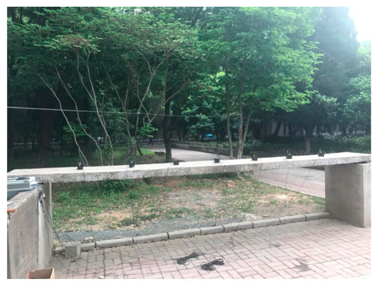
Figure 1.
Reinforced concrete (RC) Slab.
From July 1, 2017 to June 30, 2018, the RC slab was monitored for one year under natural environmental conditions and environmental temperature and vibration data were acquired. As shown in Figure 2, 45 measurement points were uniformly located on the top and bottom surface of the slab. A laser thermometer was utilized to measure the surface temperature, which allowed an error of 0.5 °C in the range of 0–100 °C. The temperature measurement and the vibration testing were carried out at the same time. Moreover, the time interval of the temperature measurement was about 15 min and vibration testing data from all sensors were captured almost simultaneously.
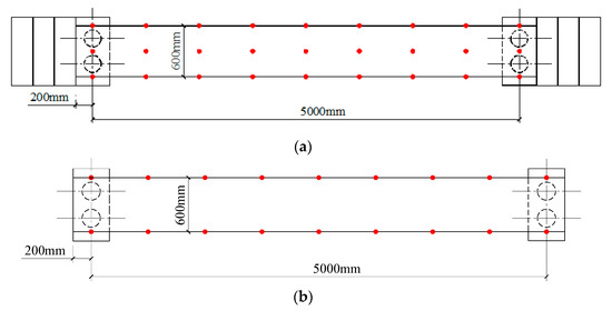
Figure 2.
Locations of temperature measurement points. (a) Top surface. (b) Bottom surface.
The acceleration data was captured by a DH5922 vibration testing system which has the advantages of light mass and convenient use etc. The operation temperature of acceleration acquisition instrument ranges from 0 °C to 60 °C. It is also a universal dynamic signal test and analysis system which can complete the testing and analysis of stress, strain, vibration, shock, acoustics, temperature, pressure, flow, force, torque, voltage and current, etc. The instrument has 16 24-bit IEPE input channels which are equipped with an anti-mixing filter, and supports sampling frequency up to 51.2k Hz. The system was connected with the acceleration sensor by L5 coaxial extension wire and placed in the center of the equal dividing line to collect the acceleration signal. The operation temperature of acceleration sensor ranged from −40 °C to 80 °C and its tolerance was ±1%. The acceleration sensor locations and vibration testing system are shown in Figure 3.
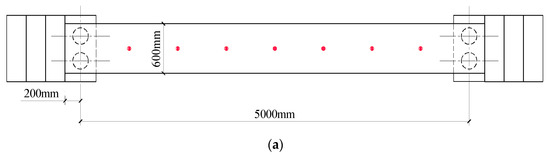
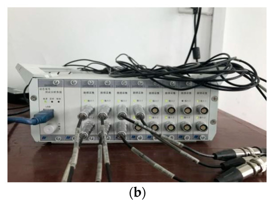
Figure 3.
Layout of acceleration sensors and vibration testing system. (a) Acceleration sensors. (b) Vibration testing system.
Monitoring for one year was performed and 180 sets of data were acquired. The monitoring temperature ranged from 0 to 55 °C, and it was found that the temperatures on the top surface vary little and the same phenomenon occurs on the bottom surface, so the average top and bottom surface temperature were calculated based on the acquired temperatures of the top and bottom surface. Then the average temperature was calculated based on the acquired average top and bottom surface temperature. Figure 4 shows the surface temperature of the slab. Typical acceleration history in time and frequency are shown in Figure 5.
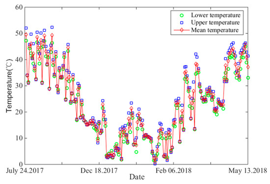
Figure 4.
Temperature variations of RC slab.
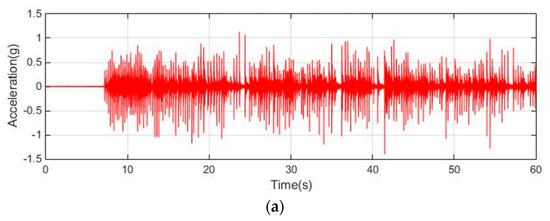
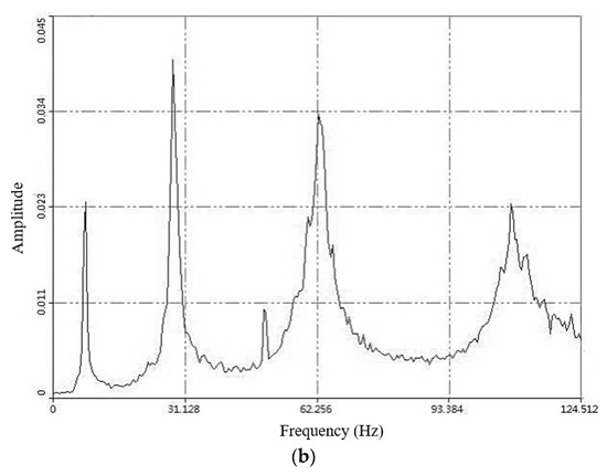
Figure 5.
Acceleration history and power spectral density. (a) Acceleration history. (b) Power spectral density.
2.2. Variations of Natural Frequencies
In this paper, the modal parameters, natural frequencies, damping ratios and mode shapes, were acquired for the investigation of the dynamic characteristics of the RC slab which should be estimated by a monitoring system based on the output-only data. However, it is difficult to excite the structure with a known force and the environmental excitation may not easily cause vibrations, so a force hammer was used for the vibration testing. The acceleration history data was analyzed by fast Fourier transform (FFT), and the mode shapes of the RC slab were extracted and shown in Figure 6.
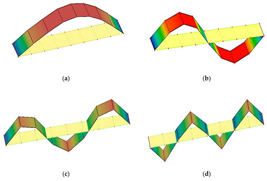
Figure 6.
First four-order mode shapes. (a) 1st mode. (b) 2nd mode. (c) 3rd mode. (d) 4th mode.
During the one-year period, 30 separate days were selected for the vibration testing which included the lowest temperatures in January 2018 and the highest in July 2017 in a year. The vibration testing was carried out periodically, once every two hours, from 8:00 am to 6:00 pm each day, because the mean temperature changes slowly from 6:00 pm to 8:00 am of the next day.
The first four natural frequencies vs. date are plotted as Figure 7 and the maximum and minimum frequencies are listed in Table 1. It can be seen that the highest temperatures and the lowest natural frequencies were in July 2017. The contrary phenomenon occurred in January 2018. The maximum variation range was 16.52% for the first natural frequency.
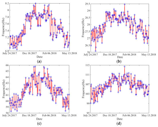
Figure 7.
Frequencies vs. test date. (a) 1st mode. (b) 2nd mode. (c) 3rd mode. (d) 4th mode.

Table 1.
The maximum and minimum natural frequencies.
The first four natural frequencies of the slab are plotted as functions of temperature in Figure 8 (degrees Celsius is specified in this paper) and it can be seen that temperature is one of the main factors affecting the eigenfrequency of the RC slab. When the temperature rises, the eigenfrequency decreases gradually, and there is a significant linear negative correlation between temperatures and natural frequencies. The linear fitting coefficients R2 of natural frequencies and temperatures for the first four modes of the RC slab are 0.898, 0.802, 0.817 and 0.800, respectively, implying that there is a good linear correlation between natural frequencies and temperatures.
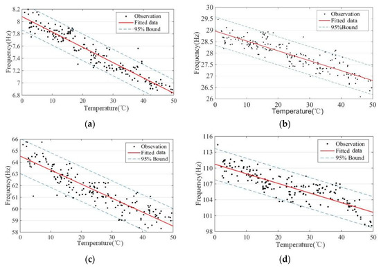
Figure 8.
Frequencies vs. temperature. (a) 1st mode. (b) 2nd mode. (c) 3rd mode. (d) 4th mode.
2.3. Variation of Damping Ratios
Based on the theory of structural dynamics, that the damping in the RC slab is proportional and viscous, the first four damping ratios are extracted and the relationships between temperature variations and modal damping ratio are shown as in Figure 9.
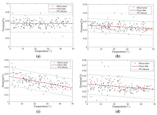
Figure 9.
Damping ratio vs. temperature. (a) 1st mode. (b) 2nd mode. (c) 3rd mode. (d) 4th mode.
It can be observed that the damping ratio decreases with the increase of temperature. The linear fitting coefficients of damping ratios and temperatures for the first four modes of RC slab were 0.0954, 0.0647, 0.3795, and 0.298, respectively. It was found that the first modal damping was relatively not sensitive to the temperature, and the other three modes had a negative correlation with temperature. This result was probably due to the fact that a linear viscous model was used. For solids and especially for concrete the models of dissipations to be used are different [34,35].
2.4. Variation of MAC
In damage detection, modal assurance criterion (MAC), which ranges from 0 to 1, is often used in automatically pairing and comparing the analytical and experimental mode shapes, here 1 and 0 mean a perfect correlation and no correlation, respectively.
In the paper, MAC is defined as [36]:
where is the experimental mode shape at the k-th vibration testing and is the analytical mode shape, which are adopted as a baseline mode shape.
The MAC values of the first four modes with respect to temperature are shown in Figure 10, whose variation ranges are (0.985, 1), (0.985, 1), (0.974, 1) and (0.975, 1), respectively. The obtained results show that all the MAC values are bigger than 0.97 and very close to unity, which implies that there is no clear correlation between MAC value and temperature, and the mode shape is less affected by environmental factors. Because there is a lower test precision for the high-mode modal shape than the low-step modal shape, the discretization degree of the MAC value is higher than the low-mode modal shape.
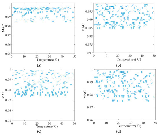
Figure 10.
MAC vs. mean temperature. (a) 1st mode. (b) 2nd mode. (c) 3rd mode. (d) 4th mode.
3. Mathematical Model
3.1. Theoretical Derivation
The variations of environmental temperature have an important influence on the mechanical properties of structural materials, especially elastic modulus. The elastic modulus of concrete decreases with the increase of environmental temperature, which leads to a decrease in eigenfrequency. Here, a simply supported beam is chosen for the investigation of the influence mechanism of temperature on structural modal characteristics. Span, elastic modulus, area of cross section, moment of inertia of cross section and uniform mass of the simply supported beam are expressed by L, E, A, I and respectively.
The n-th eigenfrequency of the simply supported beam is [37]:
The rate of change of eigenfrequency can be determined by:
where δ represents an increment in corresponding variables. When temperature changes by δt, the changes of the relative parameters are as follows, respectively:
where is the temperature coefficient of elastic modulus, which is an undetermined parameter; is the linear thermal expansion coefficient of materials. is the same grade of and it can be neglected. The three coefficients are put in the Equation (3), and it can be rewritten as:
Equation (5) can be used to estimate the eigenfrequency variation of a simply supported beam caused by temperature change. The temperature coefficient of concrete is much larger than the linear thermal expansion coefficient [38]. It can be seen that the influence of temperature dependence of elastic modulus of concrete is much greater than that of geometric size with temperature, which is the main reason for the change of natural frequencies.
3.2. Simple Linear Regression Model
The relationship between eigenfrequency and mean temperature is considered to be linear, which is shown as:
where f is the eigenfrequency; T is the temperature; k is the slope coefficient; and b is intercept. The simple linear regression model of each mode is shown in Figure 11.
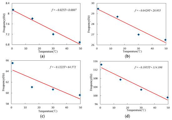
Figure 11.
Modal frequencies of linear regression model under different temperature. (a) 1st mode. (b) 2nd mode. (c) 3rd mode. (d) 4th mode.
The fitted regression line is plotted in Figure 8a–d together with the 95% confidence bounds, and the slope coefficients and intercepts for the first four natural frequencies are shown as Table 2.
Table 2.
Slope coefficients and intercepts for the first four natural frequencies.
3.3. ARX Model
The three parameters: the auto-regressive order , the exogeneous order and the pure time delay between input and output are the main features of the auto-regressive with exogenous (ARX) model. The ARX model adopted in this paper consists of an auto-regressive output and an exogeneous input part, which is shown as follows [39]:
where is the eigenfrequency at time instant , which is the output; is the temperature at time instant , which functions as the input; is the equation error, which functions as the unknown disturbances during the input–output process, such as white noise.
The ARX model can be rewritten by z-transformation:
where
When the temperature input vector is , the output vector of eigenfrequency is , Equation (7) can be rewritten as:
where the mean values of and are zero if .
In general, the above equations can be expressed in the form of matrix
where
To minimize the sum of squares of the equation errors , a criterion based on the least squares method can be defined and the best estimate of the undetermined parameter is shown as:
In this paper, the (akaike information criterion) AIC is adopted, which is practical and can be used to check mode order and is defined as:
where M is the set number of experimental data; is vector to be identified; k is parameter to be identified. The function , which is based on MATLAB, can be used to calculate the AIC value in the model, if the AIC value is small, n, m, d can be the proper mode order of the system.
Equation (12) can be transformed to Equations (18) and (19), which are models with a double input function, the first is the transfer function from input signal to output signal which is shown as Equation (20), the second is the transfer function from error signal to output signal, which can be neglected here.
In the paper, three numbers can be determined based on MATLAB, n = 4, m = 2 and d = 1; the transfer functions between temperature and the first four natural frequencies are shown Equations (21)–(24).
Fitting the mean temperature and the first four natural frequencies of the RC slab, the ARX models can be plotted as Figure 12.
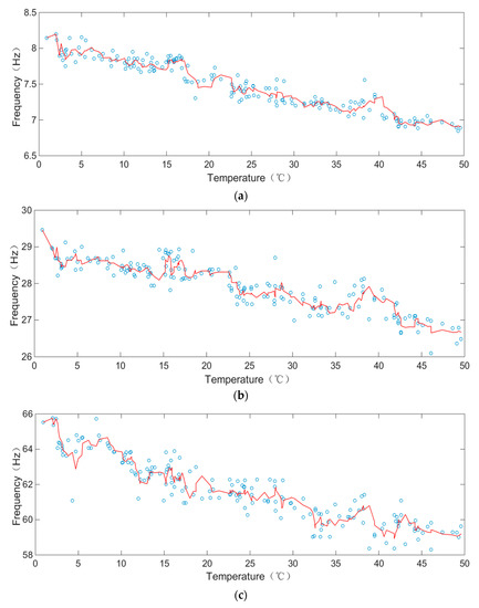
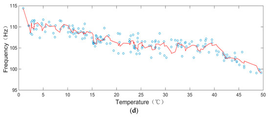
Figure 12.
Autoregressive with exogenous input (ARX) models between temperature and natural frequencies. (a) 1st mode. (b) 2nd mode. (c) 3rd mode. (d) 4th mode.
The root-mean-square error can be used to estimate the precision of the model, which can be shown as Equation (25). The less the acquired root mean squared error (RMSE) value, the better the model precision. The comparison of RMSE values of the first four natural frequencies is shown as Table 3, and it can be observed that the accuracy of the ARX model is better that of the linear regressive model.
where n is the sample size; is the experimental eigenfrequency; is the estimated natural frequencies.
Table 3.
Comparison of root mean squared error (RMSE) values between ARX model and linear regressive model.
4. Damage Identification in Test Structure
In the above experiments and analysis, the ARX model, which can reflect the relationship between natural frequencies and variations of temperature, is obtained, and it can be exploited for the damage identification problem. Theoretically, the simulated frequencies of the experimental slab can be output when the measuring temperature data are input to the model. However, if the large discrepancy is observed between the simulated and measured frequencies, something abnormal may happen and cannot be explained by temperature effects. For instance, if the measured natural frequencies are lower, the slab may be damaged. However, the significant deviation is a rather subjective criterion to judge the state of a structure. In this respect, some more objective statistical criterion needs to be discussed; if there is an abnormal change, such as a crack in structures [40,41], the procedure of damage identification will be carried out to identify whether the structure is damaged.
4.1. Statistical Criterion
The reasonable output confidence interval is determined to verify the damage identification performance of the ARX model. The finite element model of the slab is constructed to obtain some analytical natural frequencies of the intact and damaged structure. Theoretically, the analytical natural frequencies of the intact structure should be distributed within the interval. Otherwise the damage may occur in the structure. The output confidence interval, whose confidence level is , can be defined as [42]:
where is the output of the model, is found from a statistical table of the Student’s t-distribution, is the experimental value, is an asymptotically Gaussian distributed with zero mean and is a certain covariance.
For the intact structure, the first natural frequency calculated based on finite element analysis is shown in Figure 13, which indicates that the analytical natural frequencies are consistent with the output of the ARX model. The results of finite element analysis fall in the confidence interval, and the correctness of the ARX model is verified. Subsequently, the 5% and 10% uniform damage are introduced to the finite element model through the reduction of the elastic modulus of the slab and the first natural frequency is extracted. In Figure 14, for 5% uniform damage, although some frequencies fall in the interval, the ARX model can assess the health condition of the structure. Damage may occur in the structure, but the change of natural frequencies may arise from the temperature variations, and if the temperature is monitored simultaneously, the reason for the change can be determined. For 10% damage cases, the frequency data exceed the lower bound of the interval, damage occurs in the structure absolutely, which shows that the ARX model can indicate abnormal variation and has a good damage warning capability.
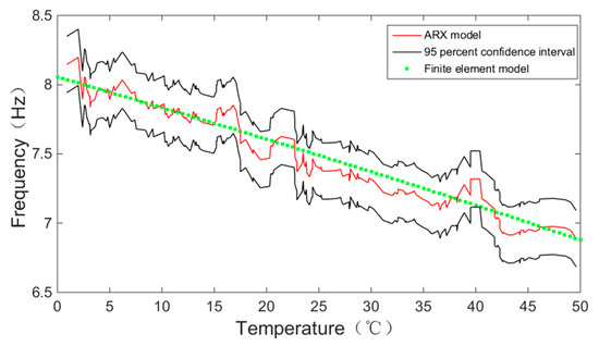
Figure 13.
Frequencies of the slab vs. temperature based on ARX model, the 95 percent confidence intervals and the finite element model.
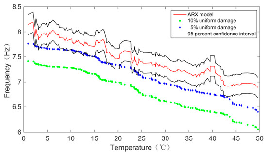
Figure 14.
Frequencies of the slab vs. temperature based on ARX model, 10% uniform damage, 5% uniform damage and the 95 percent confidence intervals.
4.2. Damage Identification Considering Temperature Variations
The linear relationship between the elastic modulus and the first natural frequencies of a simply supported beam can be obtained from Equation (2), which can be written as:
where is the span length; is the natural frequency of n-th mode; is the mass per unit length; is the sectional moment of inertia.
Consequently, the elastic modulus under the different environmental temperatures can be calculated by the experimental frequencies. The linear relationship between the elastic modulus and temperature can be obtained by least square method, and the linear fitting coefficients R2 of elastic modulus and temperatures is 0.8375, which is shown in Figure 15.
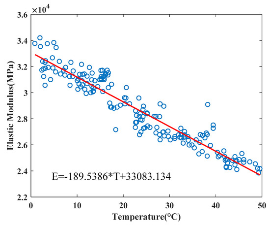
Figure 15.
Linear relationship between elastic modulus and temperature.
The linear relationship can be written as:
Then, the linear relationship of temperature vs. elastic modulus is adopted for the finite element model of the slab, and two damage cases are introduced, which are 5% and 10% uniform damage in all elements (20 °C). Statistical criterion and particle swarm optimization (PSO) are utilized to detect the damage considering the temperature effect. The PSO algorithm randomly generates the initial population named particles, which is first raised by Kennedy and Eberhar [43]. The characteristics of velocity and position are assigned to each particle which can be dynamically changed and updated by referring to the best particle in the search space. The algorithm as a powerful optimization tool aims to find the global optimal of an objective function, which is widely use in damage identification [44].
The position and velocity of each particle are updated by Equations (29) and (30) respectively, which are shown as follows:
where i stands for the i-th particle; t is the number of current iterations; c1 = c2 = 2 mean the learning factors; and are random constants in the range of [0, 1]; gbest and pbest are the global optimal particle and optimal position respectively. is the inertia weight. The objective function can be defined as:
where and are the j-th analytical and experimental natural frequency respectively; MACj is the j-th Modal Assurance Criterion (Equation (1)), nmod is the number of modes. The flowchart and identification results are shown in Figure 16 and Figure 17, respectively.
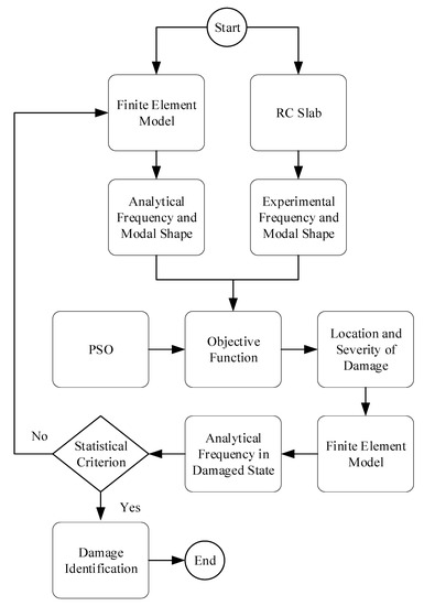
Figure 16.
The flowchart of damage identification.
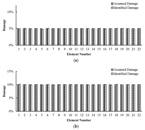
Figure 17.
Results of damage identification. (a) 5% uniform damage (20 °C). (b) 10% uniform damage (20 °C).
From Figure 17 it can be seen that the damage of the RC slab can be precisely located and accurately quantified. In addition, as shown in Table 4, the first analytical frequency of the slab in damaged state does not exceed the confidence interval, so it is evident that the proposed damage identification method is verified and is of good performance.
Table 4.
Determination of damage using statistical criterion.
5. Conclusions
In this paper, a method that can distinguish natural frequencies changes due to normal temperature variations from abnormal damage is presented. Based on the vibration testing of a RC slab for one year, the relationship between temperature and test data was analyzed. The linear regressive and ARX models were established, and it was concluded that if the experimental natural frequency lies outside the confidence intervals, it was likely that the slab was damaged. Moreover, two simulated cases are constructed and PSO is adopted to identify the location and severity of the specified damage successfully.
(1) The vibration testing of a laboratory simply supported RC slab has been performed for one year. During the period, temperatures and accelerations at different locations were monitored, and the variations of temperatures and natural frequencies were acquired. It was found that natural frequencies and damping ratios decrease with the increase of temperatures for the first four modes and there was no actual relation with MAC and temperature.
(2) The mathematical derivation of a simply supported beam was performed and it was found that the influence of temperature dependence on the elastic modulus of concrete was the main reason for the change of natural frequencies. The relationship between the elastic modulus and the temperature was obtained by deducing the equation, and the specific parameters of the relationship between the temperature and the elastic modulus were obtained by analyzing the measured data.
(3) The simple linear regressive model and the ARX model were constructed based on the vibration testing results, by analyzing the RMSE values of the model and measured data, it was found that the precision of the ARX model was better than that of the linear regressive model.
(4) An objective statistical method based on ARX model was presented to detect and identify the location and severity of the simulated damage. A confidence interval was constructed to estimate the disturbance of natural frequencies due to temperature and two simulated damage cases were set up. PSO was adopted to identify the damage and validate the proposed model, and it was found that the method in this paper can distinguish the variations of natural frequencies due to normal temperature variations from those variations due to abnormal reasons such as structural damage.
Author Contributions
Conceptualization, software, validation, resources, data curation, writing-original draft preparation, must be acknowledged to Z.W. Methodology, formal analysis, project administration, funding acquisition, must be acknowledged to M.H. Supervision must be acknowledged to J.G. All authors have read and agreed to the published version of the manuscript.
Funding
There is no funding for the paper.
Conflicts of Interest
The authors declare that there are no conflicts of interest regarding the publication.
References
- Adedayo, R.A.; Fauzi, Z.; Sathyajith, M. Sustainable energy towards air pollution and climate change mitigation. J. Environ. Eng. Landsc. 2020, 260, 109978. [Google Scholar]
- Cotana, F.; Vittori, S.; Marseglia, G.; Medaglia, C.M.; Coccia, V.; Petrozzi, A.; Nicolini, A.; Cavalaglio, G. Pollutant emissions of a biomass gasifier inside a multifuel energy plant. Atmos. Pollut. Res. 2019, 10, 2000–2009. [Google Scholar] [CrossRef]
- Marseglia, G.; Medaglia, C.M.M.; Petrozzi, A. Experimental tests and modeling on a CHP biomass plant. J. Energ. 2019, 12, 2615. [Google Scholar]
- Manni, M.; Coccia, V.; Nicolini, A.; Marseglia, G.; Petrozzi, A. Towards Zero Energy Stadiums: The Case Study of the Dacia Arena in Udine, Italy. Energies 2018, 11, 2396. [Google Scholar] [CrossRef]
- Requena-Garcia-Cruz, M.-V.; Morales-Esteban, A.; Durand-Neyra, P.; Estêvão, J. An index-based method for evaluating seismic retrofitting techniques. Application to a reinforced concrete primary school in Huelva. PLoS ONE 2019, 14, e0215120. [Google Scholar] [CrossRef] [PubMed]
- Marseglia, G.; Rivieccio, E.; Medaglia, C.M. The dynamic role of Italian energy strategies in the worldwide scenario. Kybernetes 2019, 48, 636–649. [Google Scholar] [CrossRef]
- Moaveni, B.; Behmanesh, I. Effects of changing ambient temperature on finite element model updating of the Dowling Hall Footbridge. Eng. Struct. 2012, 43, 58–68. [Google Scholar] [CrossRef]
- Moorty, S.; Roeder, C.W. Temperature?Dependent Bridge Movements. J. Struct. Eng. 1992, 118, 1090–1105. [Google Scholar] [CrossRef]
- Liang, Y.; Li, N.; Song, G.; Li, H. Damage Diagnosis under Environmental and Operational Variations Using Improved Restoring Force Method. Earth Space 2014 2015, 690–702. [Google Scholar] [CrossRef]
- Del Grosso, A.; Lanata, F. A long-term static monitoring experiment on R.C. beams: Damage identification under environmental effect. Struct. Infrastruct. Eng. 2013, 10, 911–920. [Google Scholar] [CrossRef]
- Li, J.; Law, S.; Hao, H. Improved damage identification in bridge structures subject to moving loads: Numerical and experimental studies. Int. J. Mech. Sci. 2013, 74, 99–111. [Google Scholar] [CrossRef]
- Yarnold, M.; Moon, F. Temperature-based structural health monitoring baseline for long-span bridges. Eng. Struct. 2015, 86, 157–167. [Google Scholar] [CrossRef]
- Chang, K.-C.; Kim, C.-W.; Kawatani, M. Feasibility investigation for a bridge damage identification method through moving vehicle laboratory experiment. Struct. Infrastruct. Eng. 2013, 10, 328–345. [Google Scholar] [CrossRef]
- Doebling, S.; Farrar, C.; Prime, M.; Shevitz, D. Damage Identification and Health Monitoring of Structural and Mechanical Systems from Changes in Their Vibration Characteristics: A Literature Review; Los Alamos National Lab: Los Alamos, NM, USA, 1996. [CrossRef]
- Doebling, S.W.; Farrar, C.R.; Prime, M. A Summary Review of Vibration-Based Damage Identification Methods. Shock. Vib. Dig. 1998, 30, 91–105. [Google Scholar] [CrossRef]
- Hao, H.; Xia, Y. Vibration-based Damage Detection of Structures by Genetic Algorithm. J. Comput. Civ. Eng. 2002, 16, 222–229. [Google Scholar] [CrossRef]
- Deraemaeker, A.; Preumont, A. Vibration based damage detection using large array sensors and spatial filters. Mech. Syst. Signal Process. 2006, 20, 1615–1630. [Google Scholar] [CrossRef]
- Boonlong, K. Vibration-Based Damage Detection in Beams by Cooperative Coevolutionary Genetic Algorithm. Adv. Mech. Eng. 2014, 6, 624949. [Google Scholar] [CrossRef]
- Nandan, H.; Singh, M.P. Effects of thermal environment on structural frequencies: Part II—A system identification model. Eng. Struct. 2014, 81, 491–498. [Google Scholar] [CrossRef]
- Alampalli, S. Influence of in-service environment on modal parameters//Proceedings-SPIE The International Society For Optical Engineering. SPIE Int. Soc. Opt. 1998, 1, 111–116. [Google Scholar]
- Peeters, B.; Maeck, J.; De Roeck, G. Vibration-based damage detection in civil engineering: Excitation sources and temperature effects. Smart Mater. Struct. 2001, 10, 518–527. [Google Scholar] [CrossRef]
- Zhao, J.; DeWolf, J.T. Dynamic Monitoring of Steel Girder Highway Bridge. J. Bridg. Eng. 2002, 7, 350–356. [Google Scholar] [CrossRef]
- Xu, Z.-D.; Wu, Z. Simulation of the Effect of Temperature Variation on Damage Detection in a Long-span Cable-stayed Bridge. Struct. Health Monit. 2007, 6, 177–189. [Google Scholar] [CrossRef]
- Martins, N.; Caetano, E.; Diord, S.; Magalhães, F. Cunha, Álvaro Dynamic monitoring of a stadium suspension roof: Wind and temperature influence on modal parameters and structural response. Eng. Struct. 2014, 59, 80–94. [Google Scholar] [CrossRef]
- Huang, M.; Gül, M.; Zhu, H.-P. Vibration-Based Structural Damage Identification under Varying Temperature Effects. J. Aerosp. Eng. 2018, 31, 04018014. [Google Scholar] [CrossRef]
- Jin, C.; Jang, S.; Sun, X.; Li, J.; Christenson, R. Damage detection of a highway bridge under severe temperature changes using extended Kalman filter trained neural network. J. Civ. Struct. Health Monit. 2016, 6, 545–560. [Google Scholar] [CrossRef]
- Jiao, Y.; Liu, H.; Cheng, Y.; Wang, X.; Gong, Y.; Song, G. Fuzzy Neural Network-Based Damage Assessment of Bridge under Temperature Effect. Math. Probl. Eng. 2014, 2014, 1–9. [Google Scholar] [CrossRef]
- Ni, Y.-Q.; Hua, X.; Fan, K.; Ko, J. Correlating modal properties with temperature using long-term monitoring data and support vector machine technique. Eng. Struct. 2005, 27, 1762–1773. [Google Scholar] [CrossRef]
- Farrar, C.R.; Doebling, S.W.; Cornwell, P.J. Variability of Modal Parameters Measured on the Alamosa Canyon Bridge; Los Alamos National Lab: Los Alamos, NM, USA, 1996.
- Sohn, H.; Dzwonczyk, M.; Straser, E.G. An experimental study of temperature effect on modal parameters of the Alamosa Canyon Bridge. J. Earthq. Eng. Struct. D 1999, 28, 879–897. [Google Scholar] [CrossRef]
- Xia, Y.; Hao, H.; Zanardo, G.; Deeks, A. Long term vibration monitoring of an RC slab: Temperature and humidity effect. Eng. Struct. 2006, 28, 441–452. [Google Scholar] [CrossRef]
- Liu, H.; Wang, X.; Jiao, Y. Effect of Temperature Variation on Modal Frequency of Reinforced Concrete Slab and Beam in Cold Regions. Shock. Vib. 2016, 2016, 1–17. [Google Scholar] [CrossRef]
- Zhou, G.-D.; Yi, T.-H. A Summary Review of Correlations between Temperatures and Vibration Properties of Long-Span Bridges. Math. Probl. Eng. 2014, 2014, 1–19. [Google Scholar] [CrossRef]
- Giorgio, I.; Scerrato, D. Multi-scale concrete model with rate-dependent internal friction. Eur. J. Environ. Civ. Eng. 2016, 21, 821–839. [Google Scholar] [CrossRef]
- Scerrato, D.; Giorgio, I.; Madeo, A.; Limam, A.; Darve, F. A simple non-linear model for internal friction in modified concrete. Int. J. Eng. Sci. 2014, 80, 136–152. [Google Scholar] [CrossRef][Green Version]
- Ewins, D.J. Modal Testing—Theory, Practice and Application; Research Studies Press Ltd.: Hertfordshire, UK, 2000. [Google Scholar]
- Baldwin, R.; North, M.A. A stress-strain relationship for concrete at high temperatures. Mag. Concr. Res. 1973, 25, 208–212. [Google Scholar] [CrossRef]
- Blevins, R.D.; Plunkett, R. Formulas for Natural Frequency and Mode Shape. J. Appl. Mech. 1980, 47, 461–462. [Google Scholar] [CrossRef]
- Xue, D.; Chen, Y. MATLAB Solution of Control Mathematical Problem; Tsinghua University Press: Beijing, China, 2007. (In Chinese) [Google Scholar]
- Andreaus, U.; Baragatti, P. Experimental damage detection of cracked beams by using nonlinear characteristics of forced response. Mech. Syst. Signal Process. 2012, 31, 382–404. [Google Scholar] [CrossRef]
- Placidi, L.; Barchiesi, E.; Misra, A. A strain gradient variational approach to damage: A comparison with damage gradient models and numerical results. Math. Mech. Complex Syst. 2018, 6, 77–100. [Google Scholar] [CrossRef]
- Peeters, B.; De Roeck, G. One-year monitoring of the Z24-Bridge: Environmental effects versus damage events. Earthq. Eng. Struct. Dyn. 2001, 30, 149–171. [Google Scholar] [CrossRef]
- Poli, R.; Kennedy, J.; Blackwell, T. Particle Swarm Optimisation. SSRN Electron. J. 2007, 4, 1942–1948. [Google Scholar] [CrossRef]
- Huang, M.; Lei, Y.; Cheng, S. Damage identification of bridge structure considering temperature variations based on particle swarm optimization—Cuckoo search algorithm. Adv. Struct. Eng. 2019, 22, 3262–3276. [Google Scholar] [CrossRef]


© 2020 by the authors. Licensee MDPI, Basel, Switzerland. This article is an open access article distributed under the terms and conditions of the Creative Commons Attribution (CC BY) license (http://creativecommons.org/licenses/by/4.0/).