Abstract
Basic equations for estimating the aerodynamic power captured by the Anderson vertical-axis wind turbine (AVAWT) are derived from a solution of Navier–Stokes (N–S) equations for a baroclinic inviscid flow. In a nutshell, the pressure difference across the AVAWT is derived from the Bernoulli’s equation—an upshot of the integration of the Euler’s momentum equation, which is the N–S momentum equation for a baroclinic inviscid flow. The resulting expression for the pressure difference across the AVAWT rotor is plotted as a function of the free-stream speed. Experimentally determined airstream speeds at the AVAWT inlet and outlet, coupled with corresponding free-stream speeds, are used in estimating the aerodynamic power captured. The aerodynamic power of the AVAWT is subsequently used in calculating its aerodynamic power coefficient. The actual power coefficient is calculated from the power generated by the AVAWT at various free-stream speeds and plotted as a function of the latter. Experimental results show that at all free-stream speeds and tip-speed ratios, the aerodynamic power coefficient of the AVAWT is higher than its actual power coefficient. Consequently, the power generated by the AVAWT prototype is lower than the aerodynamic power captured, given the same inflow wind conditions. Besides the foregoing, the main purpose of this experiment is to investigate the technical feasibility of the AVAWT. This proof of concept enables the inventor to commercialize the AVAWT.
1. Introduction
Albeit vertical-axis wind turbines (VAWT) are not new to subject-matter experts, it is worthwhile shedding some light on them so that readers who are not subject-matter experts can acquire some knowledge about these contrivances. Besides, the VAWT under investigation, named the Anderson VAWT (AVAWT) under the patent number US8790069 [1], is a new contraption that makes an overview of existing VAWTs relevant. The novel VAWT is different from existing ones in the sense that its blades are made of specially rolled sheet metal giving them the desired curvature for proper aerodynamic performance. It is a three-stage device with each stage made up of three specially curved blades, placed 120° from each other. The top stage leads the middle stage by a few degrees, while the same is true for the middle and bottom stages. In order to investigate the aerodynamic feasibility of a curved bladed Darrieus vertical-axis wind turbine (DVAWT) rotor, engineers at the Sandia National Laboratory of the U.S. Department of Energy (USDOE) developed a 5 m-diameter, two-bladed prototype that was mounted on the roof of their laboratory and seen to rotate on windy days. Following the aforementioned rotor was the development of a 17 m-diameter curved two-bladed rotor that was observed to perform nearly as efficiently as a horizontal-axis wind turbine (HAWT) rotor of equal capacity. A 34 m-diameter VAWT of the same type, called the test rig by Sandia, was developed thereafter and incorporated with instruments for condition monitoring and those to record weather conditions that affect its performance. Sandia also used this VAWT to validate various computer models, test airfoil designs and develop various control strategies [2]. Unlike this study that performed a wind tunnel experiment to investigate the performance of a novel VAWT, Sandia performed on-site investigations on a working VAWT.
Typically, VAWTs may have either drag-driven or lift-driven rotors. A Savonius rotor is the most common drag driven rotor. It has been used on water pumps and is inexpensive to manufacture. Savonius machines typically have low power coefficients because they are drag driven. Power coefficients of about 0.30 are typical of Savonius rotors. Additionally, they have a solidity close to unity, such that they are very heavy relative to their power production capacities, and it is also difficult to protect them from high winds [3].
A DVAWT is a lift-driven machine. Lift-driven VAWTs have almost always been used for electrical power generation. Lift-driven VAWTs typically have rotors with straight or curved blades. Some VAWTs with straight-blade rotors have a pitching mechanism, even though most lift-driven VAWTs have fixed blades. Yawing mechanisms are not needed on VAWTs, since they see the wind in any direction. Rotor blades of lift-driven VAWTs are generally untwisted and have constant chords; thus, they are easy to mass-produce. VAWTs are prone to high fatigue damage because the load on each blade varies during each rotation of the rotor. They are difficult to support on separate tall towers, since a large portion of the rotor tends to be close to the ground in a region with low wind speeds. This results in less productivity, compared to a HAWT of the same capacity [3,4].
In 1988, a 100 m tall, 60 m-diameter DVAWT was installed in Canada. The 60 m-diameter VAWT ran for six years with 94% availability [3]. As stated earlier, DVAWTs work on the principle of aerodynamic lift (i.e., the wind pulls the rotor blades along). On the contrary, the traditional Holland type windmill operates on the principle of drag (i.e., the wind pushes a manmade barrier such as a rotor blade) [2]. Typically, DVAWTs have power coefficients between 0.4 and 0.42 [5]. They are not self-starting; some drag ought to be imposed on them for them to be able to be self-starting. Installation of cups or vanes on DVAWTs makes them capable of trapping the wind, thereby causing them to self-start [2,4]. Using the foregoing methods to self-start DVAWTs results in larger blades, and these methods have been abandoned. To encourage the development of the wind energy technology in the U.S., the Federal Government gave incentives such as a tax credit of 1.80 cents/KW-h of wind energy produced. The USDOE set a goal in 2008 to achieve a 20% contribution to grid power by wind energy sources by the year 2030 [2]. This is clear evidence of the fact that there is a niche for wind energy in the U.S. energy market.
VAWTs can be effectively used in urban areas where turbulent and unsteady wind is typical [6,7]. They have inherent superiority over HAWTs in severe wind conditions, because the wind enters their rotors from about any direction without yawing. A discrepancy factor of two typically exists between computational fluid dynamics (CFD) results and results of wind tunnel experiments, since the effects of a finite blade length and spoke drag are not usually considered in CFD analysis. The performance of a VAWT with a steady inflow condition is not a reflection of the actual performance of a VAWT operating in an urban environment - an upshot of the fact that wind fluctuates in an urban environment. The performance of a wind turbine (WT) depends on the cube of the speed of the inflow wind; thus, moderate fluctuations in the wind speed would result in very large fluctuations in power output [6]. The seeming stagnation in improvements on the aerodynamics of HAWTs has spurred interest in the development of large-scale VAWTs. Another factor in favor of VAWTs is the future demand for decentralized and sustainable energy supply in cities and rural communities [8]. They are suitable where HAWTs do not operate efficiently, usually at locations with high wind speeds and turbulent wind flow. VAWTs are quieter than HAWTs, which makes them suitable for use in urban areas [9,10]. Savonius VAWTs can withstand gusts due to their superior stalling behavior and are suitable for use in gusty environments. At a tip-speed ratio of unity, the power coefficient of a Savonius rotor is optimal. Modifications on the blade geometry of Savonius rotors improve their power coefficients. The power coefficient of a Savonius rotor with a 45° angle of twist is 0.3385 compared to 0.30 for rotors with untwisted blades. Two-stage Savonius rotors perform better than their three-stage counterparts [9]. Both three-bladed and two-bladed Savonius rotors exhibit high power coefficients at low tip-speed ratios.
Curved DVAWTs with troposkein shapes are prone to nearly tensile loads and minimal bending moments on their rotor blades. They operate at distinct angles of attack at different azimuth angles and are subjected to cyclic aerodynamic loads that can result in fatigue [10]. Cognizant of the aforementioned setback on the curved DVAWTs and other VAWTs, experimental investigations and numerical simulations to ascertain their suitability for use are imperative. The International Electro-Technical Commission (IEC) guidelines include well established procedures for WT testing. Based on the IEC guidelines, the service life of a WT is 20 years. Breakdowns are frequent with WTs, and such breakdowns stem from manufacturing and design errors due to underestimated fatigue loads or extreme loads. Consideration of turbulent inflow conditions during aerodynamic modeling is of paramount importance. Turbulent characteristics of inflow air may have an impact on fatigue loads experienced by WTs [11].
Blade pitching is more difficult for VAWTs than for HAWTs due to the dependence of the angle of attack of the former on the rotor azimuth angle, resulting in the existence of very few practical pitch control schemes for VAWTs [12]. Unlike some of the existing VAWTs, which may require pitch control to maximize wind energy capture, the VAWT in this study does not require pitch control for wind energy capture optimization.
Extraction of wind momentum by a VAWT occurs more during the upwind pass. Most of the VAWT’s power output is produced on the upwind pass, whereas flow momentum is considerably reduced on the downwind pass, hence resulting in a reduced power output [13]. Darrieus-type VAWTs with straight blades are less efficient than those with helically twisted blades [14].
Various numerical and analytical schemes have been implemented in a bid to investigate performance characteristics of VAWTs. Zanon et al. [15] solved potential flow equations in conjunction with integral boundary layer equations formulated for VAWT rotors, using a semi-inverse iterative algorithm. From their simulations, they inferred that VAWTs can be designed to avoid the occurrence of dynamic stall resulting from blade-vortex interaction in the downward part of rotor rotation during gusts and normal operation, and even at low tip-speed ratios [16]. Scheurich et al. [14] implemented a CFD scheme based on the vortex transport model (VTM). The VTM is based on solving Navier–Stokes (N–S) equations in terms of the vorticity and velocity. The governing momentum equation is expressed in terms of the vorticity and velocity and is the result of finding the curl of the velocity and pressure-based N–S momentum equation. In their work on the steady-state and dynamic simulations of Savonius rotors, Jaohindy et al. [16] found that the best approximations of the static torque coefficient, the dynamic torque coefficient and the power coefficient were obtained using the shear stress transport-k-ω model rather than the k-ε turbulence model. At startup, dynamic torque coefficient curves of a Savonius rotor oscillate around fixed values in polar coordinates [16]. There is a significant difference between simulated and experimental values of the power coefficient of a DVAWT at high tip-speed ratios, even though simulation and experimental power coefficient values follow the same trend as the tip-speed ratio varies [17]. The power coefficient of a Darrieus-type VAWT peaks at tip-speed ratios between 3 and 4 and drops for tip-speed ratios greater than 4 for both CFD simulation and experimental results, with values of the former being slightly higher than those of the latter (see Figure 18 in [18]).
This study uses an experimental approach to investigate the performance of the novel AVAWT [1]. Unlike CFD simulations performed by some of the above cited researchers, which were based on two or three tip-speed ratios, this study investigates performance characteristics of the novel AVAWT over a broad range of tip-speed ratios.
2. Basic Equations of Fluid Dynamics
Stating without proof, for baroclinic flows, the integral of N–S equations [19,20,21] results in the Bernoulli’s equation given by
where is the magnitude of the fluid velocity, is the fluid pressure, is the density of the fluid, is the gravitational acceleration, is the elevation from a fixed point and is a constant. For a one-dimensional (1-D) baroclinic flow, , where is the free-stream speed of the fluid, and , yielding
Applying Equation (2) to stations 0 and 1 in Figure 1 yields , which, on further simplification, yields and
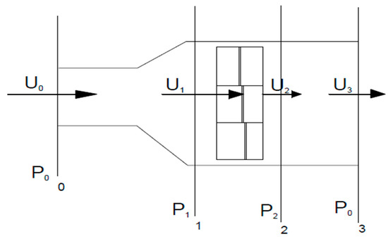
Figure 1.
Control volume of the AVAWT.
Applying Equation (2) to stations 2 and 3 in Figure 1 yields , which, on further simplification, yields and
Adding Equations (3) and (4) yields
Applying Equation (2) to stations 1 and 2 in Figure 1 yields , which, on further simplification, yields and
Adding Equations (5) and (6) yields
Momentum is recovered far downwind the VAWT due to the turbulence of the atmospheric boundary layer; thus, . Equation (7) then becomes , which, on further simplification, yields the pressure drop across the VAWT:
The wind power captured is calculated from the rate of change of the kinetic energy of the wind:
where is the mass flow rate, in which is the area of the AVAWT seen by the wind. Equation (9) then becomes
The total energy borne by the wind seen by the VAWT is given by
The power coefficient Cp is given by
3. Experiment
The purpose of this experiment is multipronged: namely, to investigate the technical feasibility of the AVAWT, to determine the power coefficient of the AVAWT, to investigate its dependence on the free-stream speed and tip-speed ratio and to investigate the dependence of the torque and power generated by the AVAWT on the free-stream speed and tip-speed ratio.
3.1. Experimental Procedures
The IEC standard number IEC61400-12-1 requires that on-site measurements of electric power generated by wind turbines be made at various wind speeds. Based on the aforementioned requirement, the power generated by the AVAWT rotor is measured at various free-stream speeds. It is worth noting that the apparatus used in this experiment consists of a 55.88 cm × 60.96 cm × 182.88 cm custom-made plywood wind tunnel, a 17.78 cm-diameter × 41.91 cm high AVAWT rotor, a Benetech hotwire anemometer (model: GM 8903 with a resolution of ±0.1 m/s and a memory of 350 records), a Hylec MS 6252 digital anemometer with a resolution of ±0.1 m/s, a Torquesense model RWT421-DD-KG torque transducer with a maximum torque range of 17.5 Nm, a steel ruler, a try-square, a Lenovo Ideapad P400 touch-screen laptop computer and a Canon PowerShot A570IS digital camera. The torque transducer measures the torque, power output and rotational speed in RPM.
Prior to carrying out the experiment, the setting of the fan used on the wind turbine was calibrated by measuring the speed of air (free-stream speed) at the center of the wind tunnel without the AVAWT rotor in place, using a hot wire anemometer, as shown in Figure 2. The free-stream speed was measured for each of the 12 settings on the fan motor’s variable speed drive. All observations were recorded. Experiments were carried out after necessary safety precautions were followed. All view windows were firmly shut; the fan end of the wind tunnel was provided with a protective wire gauze screen to prevent users from being injured by rotating equipment. Figure 3 and Figure 4 depict the setup of the experiment.
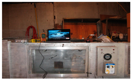
Figure 2.
Setup for the calibration of the fan air flow in terms of m/s.
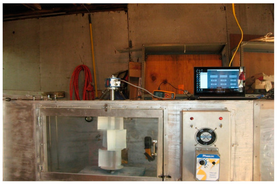
Figure 3.
Setup for measuring AVAWT performance parameters.
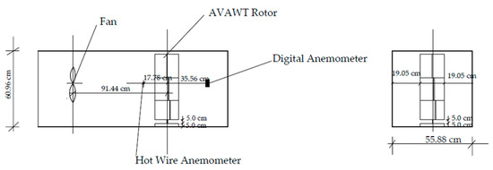
Figure 4.
Experimental setup showing measurements.
The AVAWT rotor was installed in the wind tunnel, as shown in Figure 3 and Figure 4, and was coupled with the torque transducer. The hotwire anemometer was placed at a distance of one rotor diameter upstream the AVAWT, strategically located to measure the free-stream speed at the center of the wind tunnel, while the digital anemometer was placed two rotor diameters downstream the AVAWT. All leads from measuring instruments to the laptop were connected and the setup was put on by selecting the fan speed and turning on the fan motor. All readings were taken and tabulated.
3.2. Observations
The average ambient temperature of the test compartment was about 14.9 °C at 1 atm. There was no provision for temperature control in the compartment, since this experiment was carried out in a storage hut.
It is worth noting that the fan used in this experiment has 12 speed settings; seven of the speed settings lie between 1.77 and 3.3 m/s. These speed settings imparted no rotation on the AVAWT; so their results were discarded. Recorded measurements of various parameters at corresponding free-stream speeds are shown in Table 1. Figure 5 is a calibration curve of the wind tunnel’s fan rheostat. It is a non-linear curve; thus, the relationship between the fan rheostat setting and the free-stream speed is non-linear. Only fan settings 8–12 resulted in free-stream speeds that caused the AVAWT rotor to rotate. Table 2 contains estimated induction factors at the AVAWT inlet and outlet.

Table 1.
Experimental Data.
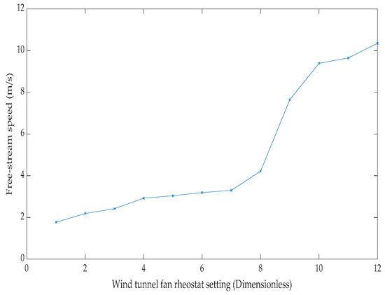
Figure 5.
Wind tunnel fan calibration profile.
Table 2.
Estimates of the induction factor.
3.3. Precision
Torque transducer measurements are within a margin of accuracy of ±0.25%. Hotwire anemometer measurements are within a margin of accuracy of ±0.3% and digital anemometer readings are within a margin of accuracy of ±2.0%.
3.4. Calculations
The angular speed of the AVAWT rotor is calculated from the measured RPM:
The rotational power is calculated from the angular speed and the measured torque T:
The actual power is reckoned from the measured electrical power and the rotational power:
The aerodynamic power is given by Equation (10):
The actual and aerodynamic power coefficients and are given by
respectively. The tip-speed ratio is given by
where R is the radius of the AVAWT rotor and is its angular speed in rad/s. The induction factor a at the AVAWT inlet is given by
The average induction factor is given by
The multiplication factor on the induction factor at the AVAWT exit and the average multiplication factor are given by
respectively.
ω = π RPM/30
4. Results and Discussion
Experimental data are used to estimate the parameters expressed in Equations (8)–(23) and tabulated in Table 2, Table 3 and Table 4. Figure 6, Figure 7, Figure 8, Figure 9, Figure 10, Figure 11 and Figure 12 depict graphs plotted from experimental results. The average induction factor calculated from experimental measurements of upwind and downwind free-stream speeds using Equations (20) and (21) is 0.642 0.0876 and the downwind speed can be expressed as , where is an average value estimated from measured upwind and downwind speeds using Equations (22) and (23) and is 1.34 0.1122. Thus, the AVAWT rotor inlet and outlet air speeds are given by
respectively.
Table 3.
Calculated angular speed, rotational power and tip-speed ratio.
Table 4.
Calculated actual power, aerodynamic power and power coefficients.
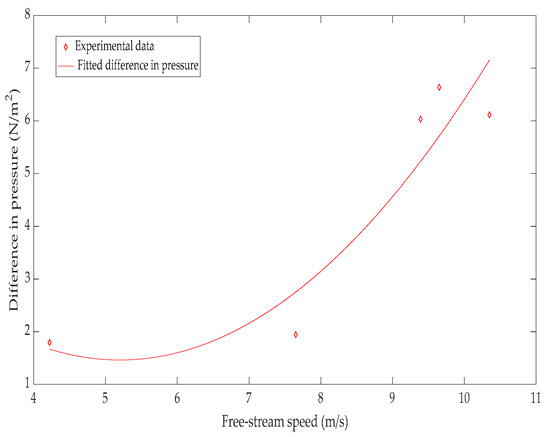
Figure 6.
Difference in pressure as a function of the free-stream speed.
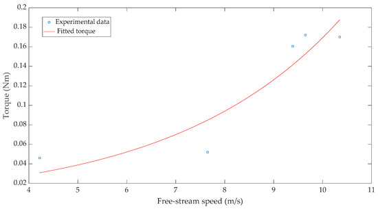
Figure 7.
Measured torque as a function of the free-stream speed.
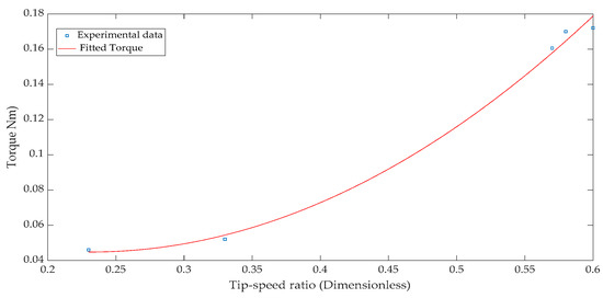
Figure 8.
Measured torque as a function of the tip-speed ratio.
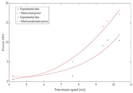
Figure 9.
Power output as a function of the free-stream speed.
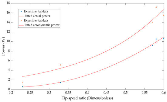
Figure 10.
Power output as a function of the tip-speed ratio.
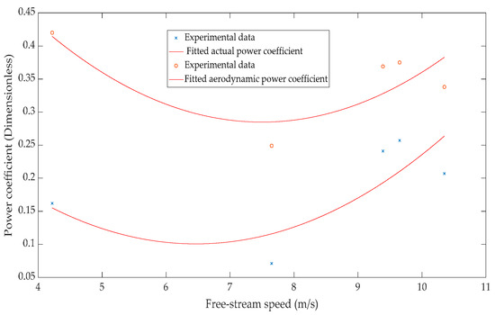
Figure 11.
Power coefficient as a function of the free-stream speed.
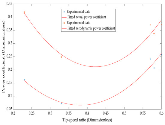
Figure 12.
Power coefficient as a function of the tip-speed ratio.
The difference in pressure between the AVAWT inlet and outlet as a function of the free-stream speed is shown in Figure 6, where rhombic points are data points calculated from experimental measurements and the best fit for the data is a quadratic curve generated using the MATLAB curve fitting tool. A coefficient of determination of 86.1% is determined for this fit, resulting in a correlation coefficient of 92.8%. The coefficients of Equations (26)–(36) have been estimated within a 95% confidence interval. The expression for the difference in pressure as a function of the free-stream speed is
It is discernible from the curve in Figure 6 that the difference in pressure across the AVAWT rotor increases parabolically with the free-stream speed.
Figure 7 depicts the measured torque as a function of the free-stream speed, where square points are experimental data points and the best fit curve is generated using the MATLAB curve fitting tool. A coefficient of determination of 86.14% is determined for this fit, resulting in a correlation coefficient of 92.81%. It is seen from the curve that the torque of the AVAWT increases exponentially with the free-stream speed. The expression for the torque as a function of the free-stream speed is
Figure 8 depicts the measured torque as a function of the tip-speed ratio, where square points are experimental data points and the best fit curve is generated using the MATLAB curve fitting tool. A coefficient of determination of 99.48% was determined for the fit, resulting in a 99.90% correlation coefficient. The curve shows that there is a quadratic relationship between the tip-speed ratio and the torque developed by the AVAWT rotor. The expression for the torque developed as a function of the tip-speed ratio is
Figure 9 depicts the measured power output as a function of the free-stream speed, where asterisks are experimental data points and the best fit curve is generated using the MATLAB curve fitting tool. The fitted actual power curve is an exponential curve whose equation is
It is discernible from the curve that the actual power generated by the AVAWT increases exponentially with the free-stream speed. A coefficient of determination of 88.21% is determined for this fit, resulting in a correlation coefficient of 93.92%. Also shown in Figure 9 is the calculated aerodynamic power as a function of the free-stream speed, where square points are data calculated from experimental measurements and the best fit curve is generated using the MATLAB plotting tool. There is a quadratic relationship between the aerodynamic power and the free-stream speed:
A coefficient of determination of 97.83 is determined for this fit, resulting in a 99.91% correlation coefficient. It is discernible from Figure 9 that the aerodynamic curve follows the same trend as the measured power curve, but the aerodynamic power values are higher than the actual power values. The aerodynamic power increases from 1.45 ± 0.1244 W at 4.22 ± 0.1300 m/s to a maximum of about 18.4 W at 10.35 ± 0.3110 m/s, while the actual power rises from 0.56 ± 0.1244 W to about 12.1 W within the same free-stream speed range. It is also discernible from Figure 9 that for free-stream speeds between about 4.6 m/s and 5.4 m/s, the aerodynamic power curve and the actual power curve nearly merge. This propensity for the curves to merge is a result of the fact that the power values are nearly equal within this free-stream speed range.
The actual power generated and the aerodynamic power as functions of the tip-speed ratio are shown in Figure 10. The aerodynamic power curve runs above the actual power curve because the aerodynamic power is higher than the actual power generated at all tip-speed ratios. This difference is evident due to friction loss on torque transducer bearings and power loss due to conversion from the kinetic energy of the rotor to resistance heating in windings of the torque transducer. Both curves in Figure 10 rise from minima at a tip-speed ratio of 0.23 ± 0.0290, at which the aerodynamic power is about 2.5 W with the actual power being 0.56 ± 0.0020 W, to maxima at a tip-speed ratio of about 0.6 ± 0.1720. At a tip-speed ratio of 0.6 ± 0.1720, the actual power read from the graph is about 10.9 W, while the aerodynamic power is about 16.8 W. The best fit for the actual power as a function of the tip-speed ratio determined with the MATLAB plotting tool is a quadratic polynomial expressed as
A coefficient of determination of 99.44% is determined for this fit, resulting in a correlation coefficient of 99.71%. An exponential curve is the best fit for the aerodynamic power curve as a function of the tip-speed ratio. The relationship between the tip-speed ratio and the aerodynamic power is given by
A coefficient of determination of 95.94% is determined for this fit using the MATLAB plotting tool, resulting in a correlation coefficient of 97.95%. It is discernible from Figure 10 that the aerodynamic power values are higher than the actual power generated. This difference in power is the result of the fact that the aerodynamic power is derived from the rate of loss of the kinetic energy of the airstream; friction loss on torque transducer bearings is not accounted for.
Figure 11 depicts the power coefficient as a function of the free-stream speed. The actual power coefficient curve is below the aerodynamic power coefficient curve. There is a scatter between experimental data and the fitted curve of the actual power coefficient; the same is true for the aerodynamic power coefficient. Both curves are parabolas with upward concavity, implying that both the aerodynamic and actual power coefficients vary quadratically with varying free-stream speeds. The actual power coefficient curve has a minimum value of about 0.1 at a free-stream speed of about 6.5 m/s, whereas the aerodynamic power coefficient curve has a minimum value of about 0.28 at a free-stream speed of about 7.3 m/s. It is discernible from Figure 11 that the aerodynamic power coefficient is higher than the actual power coefficient at all free-stream speeds. This difference in the power coefficient results from power losses due to drag, friction on torque transducer bearings and losses in generator windings. The relationship between the actual power coefficient and the free-stream speed is
A coefficient of determination of 56.25% is determined for Equation (33) using the MATLAB plotting tool, resulting in a correlation coefficient of 75%. The aerodynamic power coefficient is expressed as a function of the free-stream speed:
A coefficient of determination of 61.73% is determined for Equation (34) using the MATLAB plotting tool, resulting in a correlation coefficient of 78.57%.
Respective power coefficients as functions of the tip-speed ratio are shown in Figure 12. It is discernible from Figure 12 that the actual power coefficient curve has a minimum value of about 0.07 at the tip-speed ratio of 0.38. The relationship between the actual power coefficient and the tip-speed ratio is a quadratic polynomial:
A 93.99% coefficient of determination is determined for this fit using the MATLAB plotting tool, resulting in a correlation coefficient of 97.97%. The aerodynamic power coefficient curve has a minimum value of about 0.21 at the tip-speed ratio of about 0.42. The relationship between the aerodynamic power coefficient and the tip-speed ratio is also a quadratic polynomial:
A coefficient of determination of 89.67% is determined for this fit using the MATLAB plotting tool, resulting in a correlation coefficient of 94.67%. It is discernible from Figure 12 that the aerodynamic power coefficient curve runs above the actual power coefficient curve. This is the case because the aerodynamic power coefficient is higher than the actual power coefficient within the entire tip-speed ratio range. The aerodynamic power coefficient is an indicator of the rate of change of the kinetic energy of the airstream as it passes through the AVAWT rotor, while the actual power coefficient indicates the rate of energy conversion to electricity as the air flows past the AVAWT rotor. It is worth noting that the best way to determine the power coefficient of a WT is by measuring the actual power generated by it. Use of aerodynamic parameters to determine the power coefficient results in higher values, even when no power is generated.
Based on the results of the experiment, the average power coefficient due to the actual power generated by the AVAWT is 0.188 ± 0.0168; meanwhile, the average aerodynamic power coefficient of the AVAWT rotor is about 0.350 ± 0.0332, the power coefficient of a Savonius rotor is 0.30 [4], the power coefficient of a DVAWT is between 0.4 and 0.42 [5] and the power coefficient of a modified Savonius rotor with a 45° angle of twist is 0.3385 [9]. It is worth noting that, unlike a DVAWT that is not self-starting, the AVAWT is self-starting.
5. Wall Effects of the Wind Tunnel
Wind tunnel wall effects have an impact on the drag coefficient CD, and hence the drag on the model being tested in the wind tunnel. Damljanovic et al. [22] discovered that for blockage ratios ranging from 0.5% to 0.6% and angles of attack within , wind tunnel wall effects are negligible within measurement uncertainties. Other researchers performed numerical simulations on models with blockage ratios of 1.875% and 15% and arrived at the conclusion that the drag coefficient increased with the blockage ratio [23]. Per these researchers, it is reasonable to use the method of images in studying wall effects of a wind tunnel on the drag experienced by a model being tested in it. In this study, the method of images is used to study wind tunnel wall effects on the drag on the AVAWT rotor.
Working with a spherical model, Awbi et al. [24] discovered that the drag coefficient did not vary with the Reynolds number Re for Re ranging from 6.5 × 10⁴ to 2.2 × 10⁵, but it increased with the blockage ratio. This increase in the drag coefficient is lower for critical values of Re than it is for values less than the critical Re. The increase in the drag coefficient is lower for the critical Re because the wake is narrower, resulting in a lower wake blockage effect. The method of gathering images for blockage correction splits wind tunnel wall effects into the solid blockage due to physical dimensions of the model and the wake blockage due to the wake. Summing the two blockage factors yields the overall blockage factor :
The net effect of a wind tunnel wall is the sum of the induced speed and the wind tunnel free-stream speed [23]:
For the AVAWT rotor, the effect of blockage is to reduce the wind tunnel air speed, since the rotor rotates with energy extracted from the air that flows past it. Thus, Equation (38) becomes
After some algebraic manipulations on the Thom formula [24], the drag coefficient is given in terms of and the blockage ratio :
Based on average conditions determined in the foregoing sections, using the results from this experiment yields
which leads to
The blockage ratio for the AVAWT rotor is 0.22. By Equation (37), , and substituting Equation (42) into this expression yields . Substituting the expression for into Equation (40) yields
where by Equation (39),
Use of Equations (43) and (44) and the expression for Re yields the drag coefficient shown in Figure 13, which is a cubic polynomial with a 99.91% coefficient of determination and a correlation coefficient of 99.95%:
It is discernible from Figure 13 that the drag coefficient increases from a value of about 3.55 at Re ≅ 8.1 × 10⁴ to a peak of about 5.23 at Re ≅ 1.16 × 10⁵, after which it drops to a trough of about 5.1 at Re ≅ 1.81 × 10⁵. It then increases to a value of about 5.5 at Re ≅ 1.96 × 10⁵. The increase in the drag coefficient at Reynolds numbers between 8.1 × 10⁴ and 1.16 × 10⁵ can be the result of the thickening of the laminar boundary layer (LBL) near walls of the wind tunnel - a phenomenon that results in an increase in the skin friction between tunnel walls and the air; meanwhile, the decrease in the drag coefficient at Reynolds numbers between 1.16 × 10⁵ and 1.81 × 10⁵ can be the result of the thinning of the LBL. This thinning of the LBL results in a reduction in the skin friction between tunnel walls and the air. The slight increase after the trough can be the result of random bombardment of air particles, resulting in the narrowing of the wake of the AVAWT rotor as the Reynolds number increases. This random motion of air particles is typical of turbulent flows. Since the drag on a model is directly proportional to its drag coefficient, the effect of wind tunnel walls on the model is to increase its drag. Thus, the wind tunnel walls increased the drag on the AVAWT rotor and decreased its power output.
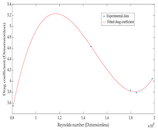
Figure 13.
Drag coefficient as a function of the Reynolds number.
6. Conclusion
Within limits of experimental errors, the average power coefficient of the AVAWT rotor based on the actual and aerodynamic powers captured is 0.269 ± 0.0250. Hence, the AVAWT rotor is less efficient than any of the aforementioned VAWTs. It is evident from this experiment that the AVAWT can generate electricity when it is coupled with a generator. The AVAWT rotor used in this experiment is many times smaller than existing VAWTs, which rendered it incapable of generating enough torque and power. Due to this shortcoming, it is unreasonable to compare its performance to those of existing VAWTs. Walls of the wind tunnel test-section also increased the drag on the AVAWT rotor, which reduced its power output. A reduction in the drag on the AVAWT rotor can be achieved by using suitable airfoil blades with rectangular slots at their trailing edges instead of the rolled sheet metal blades currently used. The slot at the trailing edge of each airfoil blade facilitates the flow of air through the blade from the high-pressure side to the low-pressure one, thereby reducing the drag and increasing the lift on the blade. This phenomenon that enhances flow from the high-pressure side to the low-pressure one through the slot at the trailing edge of an airfoil is known as boundary layer suction.
Much work remains to be done in studying performance characteristics of the AVAWT. This includes numerical simulations and quantification of the drag on the AVAWT using a wake-speed distribution at selected free-stream speeds.
Author Contributions
Conceptualization, J.A. and W.Z.; methodology, J.A.; software, J.A.; formal analysis, J.A.; investigation, J.A.; resources, W.Z.; data curation, J.A.; writing—original draft preparation, J.A.; writing—review and editing, J.A. and W.Z.; visualization, J.A.; supervision, W.Z.; project administration, W.Z. All authors have read and agreed to the published version of the manuscript.
Funding
This research received no external funding.
Acknowledgments
The authors would like to thank Bruce Anderson for his permission to use his prototype rotor in the experiment, construction of the wind tunnel for the experiment and participation in the setup of the experiment.
Conflicts of Interest
The authors declare no conflict of interest.
References
- Anderson, B.E. Enclosed Vertical Axis Fluid Rotor. 2014. Available online: www.patents.justia.com (accessed on 29 October 2019).
- Zayas, J. Scope of Wind Energy Generation Technologies. In Energy and Power Generation Handbook; Rao, K.R., Ed.; Chapter 7; ASME Press: New York, NY, USA, 2011; ISBN 978-0-7918-5955-1. [Google Scholar]
- Manwell, J.F.; McGowan, J.G.; Rogers, A.L. Wind Energy Explained (Theory, Design and Applications), 2nd ed.; Chapters 1–3; Wiley: West Sussex, UK, 2011; ISBN 978-0-470-01500-1. [Google Scholar]
- Taylor, D. Wind Energy: Renewable Energy (Power for a Sustainable Future), 3rd ed.; Boyle, G., Ed.; Chapter 7; Oxford Press: Oxford, UK, 2012; ISBN 978-0-19-954533-9. [Google Scholar]
- D’Ambrosio, M.; Medaglia, M. Vertical Axis Wind Turbines: History, Technology and Applications. Master’s Thesis, Hogskolan i Halmstad, Halmstad, Sweden, 2010. [Google Scholar]
- Wekesa, D.; Wang, C.; Wei, Y.; Kamao, J.; Damao, L.A. Numerical Analysis of Unsteady Inflow Wind for Site Specific Vertical Axis Wind Turbine: A Case Study for Marsabit and Garissa in Kenya. Renew. Energy 2014, 76, 648–662. [Google Scholar] [CrossRef]
- Wekesa, D.; Wang, C.; Wei, Y.; Damao, L. Influence of Operating Conditions on Unsteady Wind performance of Vertical Axis Wind Turbines Operating within a Fluctuating Free Stream: A Numerical Study. J. Eng. Ind. Aerodyn. 2014, 135, 76–89. [Google Scholar] [CrossRef]
- Scheirich, F.; Fletcher, T.M.; Brown, R.E. Simulating the Aerodynamic Performance and Wake Dynamics of a Vertical Axis Wind Turbine. Wind Energy 2010, 14, 159–177. [Google Scholar] [CrossRef]
- Khan, J.; Rhaman, M. Stress Analysis of Various Shaped Blade of Savonius Wind Turbine. In Proceedings of the ASME 2014 International Mechanical Engineering Congress and Exposition, Montreal, QC, Canada, 14–20 November 2014. [Google Scholar]
- Xisto, C.M.; Pascoa, J.C.; Leger, J.A.; Transconi, M. Wind Energy Production Using an Optimized Variable Pitch Vertical Axis Rotor. In Proceedings of the ASME 2014 International Mechanical Engineering Congress and Exposition, Montreal, QC, Canada, 14–20 November 2014. [Google Scholar]
- Mucke, T.; Kleinhans, D.; Peinke, J. Atmospheric Turbulence and its Influence on the Alternating Loads on Wind Turbines. Wind Energy 2010, 14, 301–316. [Google Scholar] [CrossRef]
- McPhee, D.; Beyene, A. The Straight-Bladed Morphing Vertical Axis Wind Turbine. In Proceedings of the ASME 2016 International Power Conference, Charlotte, NC, USA, 26–30 June 2016. [Google Scholar]
- McLaren, K.; Tullis, S.; Ziada, S. Computational Fluid Dynamics of the Aerodynamics of a High Solidity, Small Scale Vertical Axis Wind Turbine. Wind Energy 2011, 15, 349–361. [Google Scholar] [CrossRef]
- Scheurich, F.; Brown, R.E. Modelling the Aerodynamics of Vertical Axis Wind Turbines in Unsteady Wind Conditions. Wind Energy 2012, 16, 91–107. [Google Scholar] [CrossRef]
- Zanon, A.; Giannattasio, P.; Ferreirra, C.J.S. A Votex Panel Model for the Simulation of the Wake Flow Past a Vertical Axis Wind Turbine in Dynamic Stall. Wind Energy 2013, 16, 661–680. [Google Scholar] [CrossRef]
- Jaohindy, P.; Ennamiri, H.; Garde, F.; Bastide, A. Numerical Investigation of Airflow Through a Savonius Rotor. Wind Energy 2014, 17, 853–869. [Google Scholar] [CrossRef]
- Edwards, J.M.; Danao, L.A.; Howell, R.J. PIV Measurements and CFD Simulation of the performance and Flow Physics and a Small-Scale Vertical Axis Wind Turbine. Wind Energy 2015, 18, 201–217. [Google Scholar] [CrossRef]
- Ragni, D.; Ferreira, C.S.; Correali, G. Experimental Investigation of an Optimized Airfoil for Vertical Axis Wind Turbines. Wind Energy 2015, 18, 1629–1643. [Google Scholar] [CrossRef]
- Kundu, P.K.; Cohen, I.M. Fluid Mechanics, 3rd ed.; Chapter 4; Elsevier: California, USA, 2004; ISBN 978-0-12-178253-5. [Google Scholar]
- Aris, R. Vectors, Tensors and the Basic Equations of Fluid Mechanics; Chapters 4–6; Dover Publications, Inc.: Mineola, NY, USA, 1989; ISBN 0-486-66110-5. [Google Scholar]
- Graebel, W.P. Advanced Fluid Mechanics; Chapters 1–3; Elsevier: Burlington, MA, USA, 2007; ISBN 978-0-12-370885-4. [Google Scholar]
- Damljanovic, D.; Vukovic, D.; Ocokoljic, G.; Rasuo, B. A Study of Wall interference effects in Wind Tunnel Testing of a Standard Model at Transonic speeds. In Proceedings of the 30th Congress of the International Council of the Aeronautical Sciences (ICAS 2016), Daejeon, Korea, 25–30 September 2016. [Google Scholar]
- Mokhtar, W.; Hasan, M.R. A CFD Study of Wind Tunnel Wall Interference. In Proceedings of the 2016 ASEE North Central Section Conference, Mount Pleasant, MI, USA, 18–19 March 2016. [Google Scholar]
- Awbi, H.B.; Tan, S.H. Effects of Wind-Tunnel Walls on the Drag of a Sphere. ASME J. Fluids Eng. 1983, 103, 461–465. [Google Scholar] [CrossRef]


© 2020 by the authors. Licensee MDPI, Basel, Switzerland. This article is an open access article distributed under the terms and conditions of the Creative Commons Attribution (CC BY) license (http://creativecommons.org/licenses/by/4.0/).