1. Introduction
A supervised learning process is the machine learning task of training a function that maps an input to an output based on data points with known outputs. Classification is the process of predicting to which of a set of categories a new observation belongs. Thus, the purpose of classification is to achieve a model that will be able to classify the right class to an unknown pattern. However, there are an increasing number of problems where a pattern can have several labels simultaneously associated. Examples can be found in genetics [
1], image classification [
2], etc. The generalization of the classic classification is Multi-Label Learning (MLL) [
3,
4,
5,
6], where multiple labels can be assigned to each instance.
Nevertheless, in many real-world problems we may face cases where MLL is still not enough, as the degree of description of each label is different. To appoint only one dataset used in this paper, the biological experiments on yeast genes [
7] during a period of time yield different levels of gene expression in a time serie. The exact level of expression at any point in time is of less importance. What becomes really decisive is the overall expression distribution over the whole period of time. If the learning goal is to predict that distribution for a particular gene, it cannot easily fit into the MLL framework because the role of each output in the distribution is critical, and there is no division of relevant and irrelevant labels at all.
The proposal of Label Distribution Learning (LDL) appeared for first time in 2013 [
8] and was formally introduced in 2016 [
9] in order to handle ambiguity on the label side of the mapping when one instance is not mandatorily matched to one single label. The main objective of this paradigm is to respond to the question “how much does each label describe the instance?” instead of “which label can describe the instance?”.
Numerous studies have been conducted by applying the LDL framework to diverse real-life problem solving scenarios, e.g., facial age estimation [
8], pre-release prediction of crowd opinion on movies [
10], crowd counting in public video surveillance [
11], sense beauty recognition [
12], image emotion classification [
13], personality recognition on social media [
14], head pose estimation [
15], etc. Further research has focused more on the development of new learners or on the adaptation of existing ones such as: instance-based algorithms (e.g., AA-
kNN [
9]), optimization algorithms (e.g., SA-IIS, SA-BFGS [
9] or LDL-SCL [
16]), decision trees (e.g., LDL forests [
17]), deep learning algorithms (e.g., Deep Label Distribution [
18]), or ensembles strategies (e.g., Logistic boosting regression for LDL [
19], Structured random forest for LDL [
20]).
AA-
kNN [
9] has proven to be a very competitive algorithm in previous experimental studies, achieving acceptable results and allowing an explainable model [
21]. However, like any other instance-based algorithm, it suffers from several handicaps: it needs large memory requirements to store the training set, it is not efficient predicting due to the multiple computations of similarities between the test and training samples and it presents a low tolerance to noise because it uses all the data as relevant.
Nowadays, one of the main challenges of supervised learning algorithms is still how to deal with raw datasets. Data collection is usually an unsupervised process, leading to datasets with redundant information, noisy data or irrelevant features. Hence, data pre-processing is an important step in the data mining process, that can mitigate this type of problem and generate improved datasets. The purpose of this paper is to address the LDL problem from the data pre-processing stage, by applying data reduction techniques which will allow us to have a reduced representation of the original data while maintaining the essential structure and integrity [
22]. These pre-processing techniques often result in better performance of subsequent learners.
Two of the most widely used data reductions techniques are the instance selection [
23], also known as prototype selection in case of instance-based algorithms [
24], and the feature selection or reduction of the data dimensionality [
25]. The first technique focuses on finding an optimal subset of samples to optimize the performance of the learner while the main idea of the second technique is to replace the original set of features by a new subset that extract the main information and provide an accurate classification.
A few methods are available to approach the instance selection in the MLL domain [
26,
27,
28] but, to the best of our knowledge, there are no studies concerning instance or prototype selection reported in LDL. With regard to the feature selection, most of LDL algorithms are built on a simple feature space where all features are used to predict all the labels. However, in real-world applications, an instance is characterized by all labels, but some labels can only be determined by some specific features of their own. Although label-specific feature selection has been widely studied in MLL [
29,
30], the studies we can find on this subject for LDL are still scarce [
31].
Prototype selection and Label-Specific Feature Evolutionary Optimization for Label Distribution Learning, or from now ProLSFEO-LDL, is our proposal for a pre-processing algorithm adapted to LDL problems and specifically designed to mitigate the handicaps of the AA-kNN method. We provide a novel method to simultaneously address the prototype selection and the label-specific feature selection. Both pre-processing techniques can be considered as a search problem where the search space is huge. Therefore, we have devised a search method based on evolutionary algorithms [
32] that allows us to obtain a solution to both problems in a reasonable time. To this end, we have adapted elements of classical evolutionary algorithms to manage LDL restrictions, we have designed a representation of the solution and a way to measure its quality, which allows us to address both problems together.
In order to evaluate the proposal proficiency, we will compare an LDL-learner applying our ProLSFEO-LDL algorithm to the raw training set and measuring six aspects of their performance. We will repeat the experiment over 13 real-world datasets and validate the results of the empirical comparisons using Wilcoxon and Bayesian Sign tests [
33,
34,
35].
The rest of the paper is organized as follows. First, a brief review and discussion of the foundations of LDL, a description of data reduction techniques and an introduction to the evolutionary optimization process are given in
Section 2. The proposed ProLSFEO-LDL method is described in
Section 3. Then the details of the experiments are reported in
Section 4. Finally, the results and conclusions are drawn in
Section 5 and
Section 6, respectively.
2. Preliminaries
In this section, the foundations and the most relevant studies carried out on LDL (
Section 2.1), are presented. Furthermore, some basic concepts on instance selection and label-specific features selection for classification are introduced (
Section 2.2), as well as the notions needed to optimize solutions using evolutionary algorithms (
Section 2.3), providing the necessary background required to properly present the study carried out in this paper.
2.1. Foundations of Label Distribution Learning
We can formalize a LDL problem as a set of m training samples , where = is a q-dimensional vector. For each instance , the label distribution is denoted by where , such that denotes the complete set of labels. The constant c is the number of labels and is the description degree of the particular jth label for a particular ith instance . According to the definition, for each the description degree should meet the constraints and .
The solution to an LDL problem can be addressed from several perspectives. According to the selected approach, the algorithm to be developed may differ significantly, either a brand-new algorithm designed especially to deal with LDL constraints, or an adaptation of already available classification algorithms, reformulated to work with those constraints. The LDL study presented in [
9] suggested six algorithms grouped in three categories. The first one is Problem Transformation (PT), a simple way to convert an LDL problem into a Single-Label Learning or SLL [
36] problem. PT transforms the training samples into weighted single-label examples. Thus, any SLL algorithm may be applied. Two representative algorithms are PT-Bayes and PT-SVM. The second one is Algorithm Adaptation (AA), in which the algorithms are tailored to existing learning algorithms to handle directly with the label distribution. Two suitable algorithms were presented: AA-
kNN, an adaptation of the well-known
k-nearest neighbors method [
37], and AA-BP, a three-layer backpropagation neural network. Finally, Specialized Algorithms (SAs), in contrast to the indirect strategy of PT and AA, directly match the LDL problem. SA-IIS and SA-BFGS are two specialized algorithms that learn by optimizing an energy function that is based on the maximum entropy model.
Subsequent works have successfully improved the results achieved by these original algorithms through different approaches. The methods LDLogitBoost and AOSO-LDLogitBoost proposed in [
19], are a combination of the boosting method and the logistic regression applied to LDL framework. Deep Label Distribution Learning (DLDL) [
18] and LDL based on Ensemble Neural Networks (ENN-LDL) [
38] are two examples of success in the application of neural networks in LDL. Modelled on differentiable decision trees [
39], an end-to-end strategy LDL forests proposed in [
17] was used as the basis for Structured Random Forest (StructRF) [
20]. BC-LDL [
40] and DBC-LDL [
41] use the binary coding strategies to address with the large-scale LDL problem. Classification with LDL (LDL4C) [
42] is also an interesting approach when the learned label distribution model is considered as a classification model. Feature selection on LDL [
43] shows encouraging results by applying feature selection on LDL problems.
2.2. Prototype Selection and Label-Specific Feature Learning
Nowadays, one of the main challenges for supervised learning algorithms is still how to deal with raw datasets. Data pre-processing is an often unattended but important step in the data mining process [
22]. Data gathering is often a poorly monitored process, resulting in low-quality datasets. If there is a lot of irrelevant and redundant information or noisy and unreliable data, then knowledge discovery is more difficult to carry out.
Data reduction techniques [
22] allow us to obtain a reduced representation of the original data but maintaining the essential structure and integrity. Such pre-processing techniques usually lead to improved performance of subsequent learners.
A frequent problem with real datasets is their big volume, as well as the presence of noise and anomalies that complicate the learning process. Instance selection is to choose a subset of data to achieve the original purpose of a data mining application as if the whole data is used [
23]. The optimal outcome of instance selection is a stand-alone model, with a minimal data sample that can perform tasks with little or no performance degradation.
Instance selection has been successfully applied to various problem types like imbalanced learning [
44], data streams [
45], regression [
46], subgroup discover in large size datasets [
47]. The research conducted in [
48] is also of interest to investigate the impact of instance selection on the underlying structure of a dataset by analyzing the distribution of sample types. However, as of today, instance selection has not been extensively researched in the domain of MLL and to date only few methods have been made available [
26,
27,
28]. As for LDL, we have not been able to find any studies to date.
Prototype Selection [
22] methods are Instance Selection methods that expect to find training sets that offer the best ranking accuracy and reduction rates by using instances-based classifiers which consider a certain similarity or distance measure. A widely used categorization of prototype selection methods consists of three types of techniques [
24]: Condensation, where the aim is to retain border points, preserving the accuracy of the training system; Edition, where the objective is to eliminate boundary points that are considered noise or do not match their neighbors but without removing the internal points of each dataset; or Hybrid methods that try to find a small set of training data while maintaining the performance of the classifier. The best approach considering the trade-off between reduction and accuracy is usually the hybrid technique.
To name just a few successful cases when applying prototype selection, [
49] proposes a prototype selection algorithm called MONIPS that has proved to be competitive with classical prototype selection solutions adapted to monotonic classification. The experimental study presented in [
50] shows a significant improvement when prototype selection is applied to dynamic classifier and ensemble selection.
Another widely used pre-processing technique is the reduction of the data dimensionality by means of feature selection [
25]. The main idea is to replace the original set of features by a new subset that extract the main information and provide an accurate classification. However, in MLL and LDL, the strategy of selecting a set of characteristics shared by all labels may not be optimal since each label may be described by a specific subset of characteristics of their own. Label-specific feature learning has been widely studied in MLL. For instance, LIFT [
29] firstly builds specific features of each label by performing cluster analysis on its positive and negative instances, and then conducts training and testing by querying the cluster results. LLSF [
30] proposes learning label-specific features for each class label by considering pairwise (i.e., second-order) label correlations. MLFC [
51] is also a multi-label learning method, which attempts to learn the specific characteristics of each label by exploiting the correlations between them. However, the studies we can find on this subject for LDL are still scarce. LDLSF [
31] is a method inspired in LLSF adapted to deal with LDL problems by jointly selecting label-specific features, selecting common features and exploiting label correlations.
2.3. Evolutionary Optimization
Evolutionary algorithms (EAs) [
32] are stochastic search mechanisms based on natural selection notions. EAs have been applied to a broad range of problems, including search problems [
52], optimization problems [
53], and in many areas as in economics, engineering, biology, etc. The primary idea is to maintain a population of chromosomes, that represent valid solutions to the problem and which evolve over time through a process of competition and targeted variation. CHC [
54], is a well-known evolutionary model that introduces different techniques to achieve a trade-off between exploration and exploitation; such as incest prevention, reinitialization of the search process when the population converges or the search stops making progress and the competition among parents and offsprings into the replacement process.
Prototype Selection can be considered as a search problem where EAs can be applied. The search space consists of all the subsets of the training set. This can be represented by using a binary chromosome with two possible states for each gene. If the gene value is 1 then the associated instance is included in the subset, if the value is 0, this does not occur. The chromosome will have as many genes as the number of instances in the training set. EAs have been used to solve the prototype selection problem with promising results [
55,
56,
57,
58,
59].
Label-specific feature selection is a very complex task. If the original set contains
q features and
c labels, the objective is to find a
binary matrix where each
position indicates if the individual feature
will be taken into consideration to predicte the label
. Many search strategies can be used to find a solution to this problem but finding the optimal subset can be a huge time-consuming task. Therefore, it is justifiable to use an evolutionary algorithm that gives us an approximate solution in an acceptable time. Several studies have successfully applied feature reduction to multi-label problems using evolutionary algorithms [
60,
61,
62,
63], but as of today no such technique has been used to solve the label-specific feature learning problem.
3. ProLSFEO-LDL: Protoype Selection and Label-Specific Feature Evolutionary Optimization for Label Distribution Learning
ProLSFEO-LDL is an evolutionary algorithm proposal adapted to LDL specificities that combines prototype selection and label-specific feature learning.
It uses the framework of CHC where the search space will be represented by a chromosome (or individual) in which we will code the prototype selection and label-specific feature as detailed in the next
Section 3.1. Through the evolutionary algorithm described in Algorithm 1, we will optimize this initial solution until we reach a solution that meets our expectations. We start from a parent population
P of size
N, randomly initialized, to generate a new population
obtained by crossing the individuals of the parent population. The recombination method to obtain the offsprings is detailed in the
Section 3.2. Then, a survival competition is held where the best
N individuals from the parent population
P and the offspring population
are selected to compose the next generation. To determine if one individual is better than another we need to evaluate the quality of each chromosome, for this we use the fitness method described in the
Section 3.3. When the population converges or the search no longer progresses, the population is reinitiated to introduce a new diversity into the search, for this purpose we use a threshold
t to control when the reinitialization will take place, this step is explained in the
Section 3.4. The process of evolution iterates over
G generations and finally returns the best solution
B found in the search.
In the following sections, we explain in depth each part of the proposed method.
| Algorithm 1: ProLSFEO-LDL: Prototype selection and Label-Specific Feature Evolutionary Optimization for Label Distribution Learning |
![Applsci 10 03089 i001]() |
3.1. Representation of Individuals
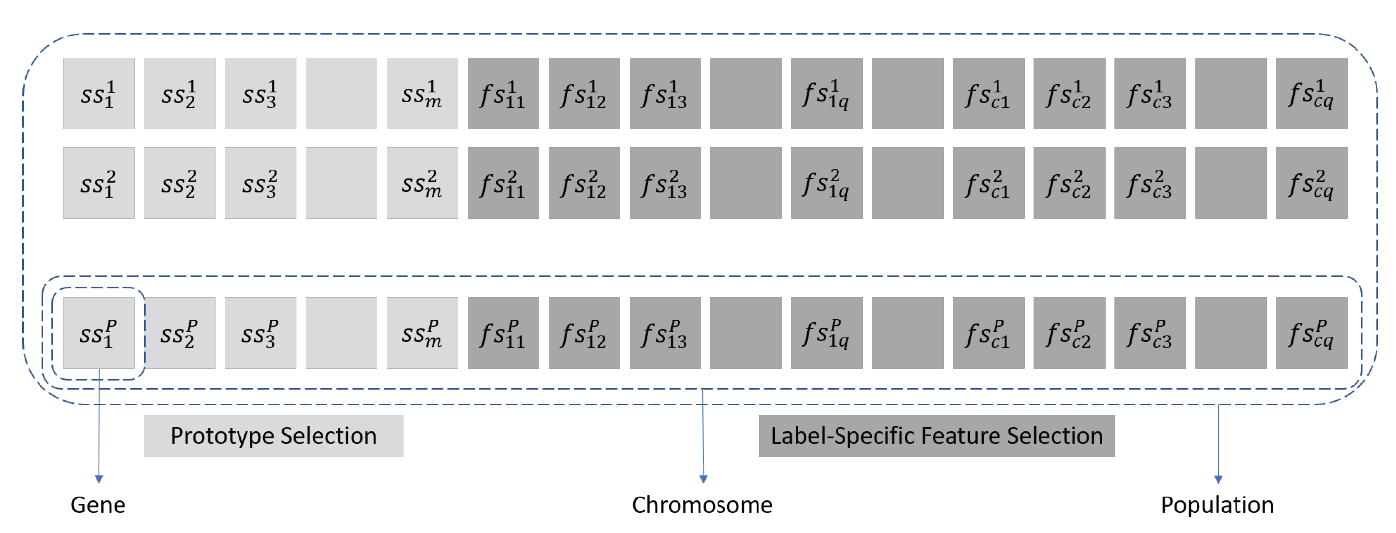
Each individual should represent the two parts of the algorithm. On the one hand, we have the first
m genes of the chromosome that represents the selection of instances, if the gene value is 1 then the associated instance is included in the subset, if the value is 0, this does not occur. And, the second part of the chromosome, consists of
genes representing the matrix of label-specific features. A graphical representation of genes, chromosome and population is exposed in
Figure 1, where genes named as
represent if the instance
i will be included in the final set or not; and genes
represent if feature
k will be taken into account to predicte the specific label
j. The initialization of the chromosomes that make up the population is randomly performed from the “discrete uniform” distribution in the closed interval
.
3.2. Crossover
The crossover operator, HUX, performs a uniform cross that randomly exchanges exactly half of the bits that differ between the two parenting chains. No mutation is applied during the recombination phase of the CHC algorithm.
3.3. Fitness Function
In order to measure the quality of a particular chromosome we need to evaluate it using a LDL learner as wrapper. As the prototype selection is focused on the optimization of the AA-kNN method, we have chosen this same learner, but with some adaptations to support the selection of features. By default AA-kNN uses all features to calculate the distance between each instance. In our adaptation, each output label j should be individually predicted using only the selected features from coded in the chromosome. The prediction obtained is then normalized so that the result is compatible with the LDL constraints.
The step sequence for evaluating a chromosome is as follows:
Create a subset of instances: the selected prototypes are coded in the first m genes of the chromosome. We create a subset T by keeping only the elements of the original training set S which have an associated gene value = 1.
Prediction phase: we use the subset T as the training set for AA-kNN. The prediction is then computed over a set merged from the test predictions of a 10-fold cross validation set (10-fcv) created from the original training set S.
Evaluation phase: in order to measure the fitness of the chromosome, we calculate the distance between the predicted label distribution and the real label distribution D using the Kullback–Leibler divergence formula , where and are the description degree of the particular jth label. In our case the fitness of the chromosome directly matchs with the KL divergence.
The objective is to minimize the fitness function.
3.4. Reinitialization
When the population converges or the search no longer progresses, the population is reinitiated to introduce a new diversity into the search. The population is considered not sufficiently diverse when the threshold L reaches 1 (line 13 in Algorithm 1). This treshold is initialized with the parameterized value t (line 4 in Algorithm 1) and decreased by 1 each time that the population is not evolving (line 12 in Algorithm 1). In such a case, only the chromosome that represents the best solution found during the search is kept in the new population, and the remaining individuals are randomly generated, filling in the rest of the population (lines 14–17 in Algorithm 1). In CHC, the typical value used for threshold t is equal to the total length of the chromosome divided by 4. In our case, due to the length of the chromosome, we will choose a lower value that allows a faster convergence.
5. Results and Analysis
This section presents the results of the empirical studies and their analyses. We will compare the results obtained by AA-
kNN with the results obtained by applying the pre-processing step ProLSFEO-LDL. In
Table 4 the best outcome for each dataset and measure is highlighted in bold. The last row is the average aggregation result of each column. The best average is also highlighted in bold. As those algorithms have been tested using 10-fcv, the performance is represented using “mean ± standard deviation”.
The Wilcoxon test and Bayesian Sign test [
33,
34] are used to validate the results of the empirical comparisons. In the Bayesian Sign test, a distribution of the differences of the results achieved using methods
L (AA-
kNN) and
R (ProLSFEO-LDL) is computed into a graphical space divided into three regions: left, rope and right. The location of most of the distribution in these sectors indicates the final decision: the superiority of algorithm
L, statistical equivalence and the superiority of algorithm
R, respectively. KEEL package [
69] has been used to compute the Wilcoxon test and the R package rNPBST [
70] was used to extract the graphical representations of the Bayesian Sign tests analyzed in the following empirical studies. The Rope limit parameter used to represent the Bayesian Sign test is 0.0001.
The outcome of both statistical tests applied to our method is represented in
Table 5 (Wilcoxon test) and
Figure 2 (Bayesian Sign test).
Comparing ProLSFEO-LDL with the standard LDL learner AA-kNN, we reach the following conclusions:
The results of the different measures shown in
Table 4 highlights the best ranking of ProLSFEO-LDL in the large majority of the datasets and measures.
The Wilcoxon Signed Ranks test corroborates the significance of the differences between our approach and AA-
kNN. As we can see in
Table 5, all the hypotheses of equivalence are rejected with small p-values.
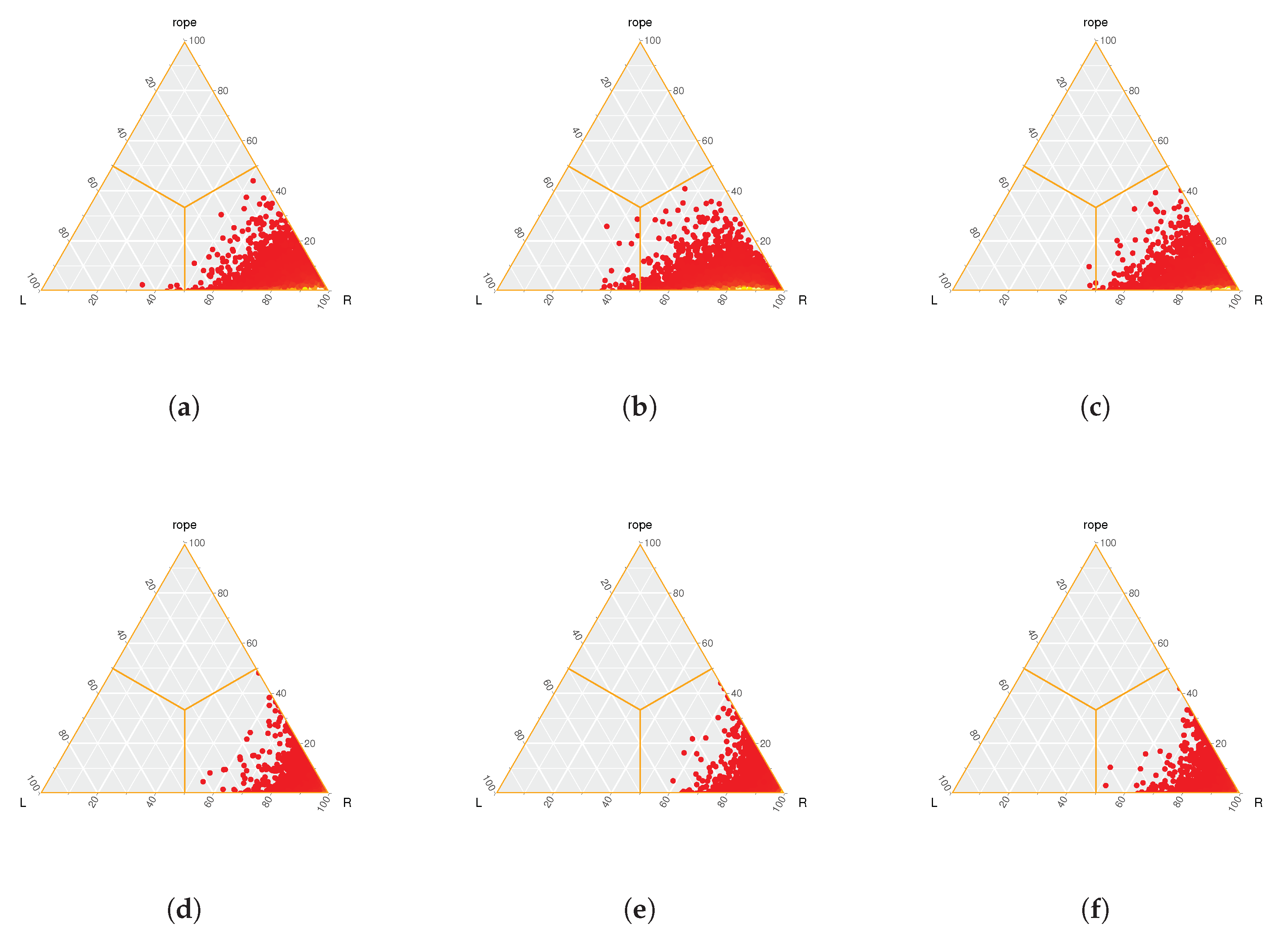
With regard to the Bayesian Sign test,
Figure 2 graphically represent the statistical significance in terms of precision between ProLSFEO-LDL and AA-
kNN. The following heat-maps clearly indicate the significant superiority of ProLSFEO-LDL, as the computed distributions are always located in the right region.
Another interesting information to analyse is the reduction ratio obtained by the proposed method. In
Figure 3 we show the percentage of selected prototypes and features with respect to the initial training set. In the case of features we represent the average percentage since each of the output labels can be represented by a different number of features.
The average percentage is around 53% for both, prototypes and features, varying more significantly for the SJAFFE and SBU_3DFE datasets where the reduction ratio decreases significantly. This percentaje of data reduction will have a huge impact in the performance of the learner. In instance-based methods like AA-kNN, the fact of handling about half of the prototypes and features, will lead to a reduction of computation time in the prediction phase.
6. Conclusions
In this paper, we proposed a novel data reduction algorithm that adapts to LDL constraints. It simultaneously address the prototype selection and the label-specific feature selection with two objectives: finding an optimal subset of samples to improve the performance of the AA-kNN learner and selecting a subset of characteristics specific for each one of the output label. Both tasks have been addressed as search problems using an evolutionary algorithm, based on CHC, to optimize the solution.
In order to verify the effectiveness of the solution designed, ProLSFEO-LDL has been applied on several real-world LDL datasets, showing significant improvements compared to the use of the raw training set. The results of the different measures highlights the best ranking of ProLSFEO-LDL, outcomes subsequently corroborated by statistical tests. In addition, the percentaje of data reduction reached leads to a significant improvement of prediction time.
In future studies we may introduce some further comparisons between already existing approaches and also make improvements to the presented proposal such as:


