1. Introduction
The liver is very important and the largest internal organ of the human body that performs very basic functions, such as detoxification of drugs, hormones, protein production, and blood filtration [
1]. Liver cancer or haptic cancer is one of the most threatening diseases. Hepatocellular carcinoma (HCC) is the most encountered, at 80% of all hepatic cancers [
2]. There are several factors that cause liver cancer, such as alcohol, smoking, obesity, etc. Diagnosis of liver cancer is not easy at an early stage [
1]. Medical diagnosis is really important and needs to be performed accurately and efficiently. Sometimes, there is a possibility of mistakes while examining such severe diseases. Therefore, an intelligent system is needed to reduce the probability of error in diagnosis [
2].
According to World Cancer Research Fund International, an American institute for cancer research (2018), liver cancer is the fifth most common cancer for men and the ninth most common cancer for women [
3]. In 2018, the number of new liver cases that were diagnosed worldwide was 840,000. Among all countries, Mongolia had the highest standardized age rate of 93.7 per 10,000 of liver cancer in 2018, followed by Egypt, with a rate of 32.2 [
4]. The “Continuous Update Project” panel considered that there is clear evidence that a greater amount of body fat and consumption of alcoholic beverages and contaminated foods with aflatoxins increase the threat of liver cancer. There is strong evidence that drinking coffee decreases the risk of liver cancer. Being physically active and consuming fish can shrink the risk of liver cancer [
4].
Liver is a major parenchymal organ of the human body that performs several functions. This means that a high amount of blood flows through the liver, which makes the liver vulnerable to the occurrence of secondary cancers. The vast majority of liver cancers originate in different organs. For effective treatments, cancers must be localized and identified accurately [
5]. Liver cancer is the second most frequent reason of death from cancer and is less common in women than in men. As age increases, the risk of liver cancer increases. Most cases are usually diagnosed in the patients who are above 75 years of age [
6]. However, there is a probability that people who belong to less developed areas in Africa and in Asia are more vulnerable to liver cancer at a younger age as compared to people in developed countries (typically around the age of 40). Approximately 83% of liver cancer cases are found in less developed geographical regions. In Europe, the Caribbean, and Latin America, the occurrence of liver cancer is the lowest. The age-standardized rate of this cancer is more than six times higher in Eastern Asia than in Northern Europe [
6].
Image processing is an area of computing that is becoming progressively prominent these days. It is applicable in various domains and can be used in the industry to regulate production, in safety systems to assess people’s biometrics, etc. [
7]. Computer-aided analysis of medical images contributes a lot in several fields of medicine, such as diagnosis, monitoring or therapy planning [
8]. Due to the aging of society and the generality of modern technologies of imaging, the number of medical images that will be processed in clinical practice is increasing [
9]. There is a great need for software tools that speed up the analysis of the medical image and make it beneficial and reproductive. An important fragment of the field is the medical image, in which image processing techniques and artificial intelligence are employed to crack problems [
9]. This work offers a computerized diagnostic system that adjusts to the field of medical imaging and aims to locate and identify cancers in liver.
Machine learning refers to training a machine to do a specific task (here, image processing) by providing it with a training data set. It incorporates several algorithms and approaches [
10]. Among them, we can choose any to analyze, which will provide better results for image classification. Results also depend on the image processing type that you are willing to adapt, as each type has its own inherent properties [
7]. For example, there is a high possibility that the cross-entropy loss function could perform better than other loss functions to give better image processing.
1.1. Literature Review
The Reference [
11] proposed a study in which liver lesions were classified into malignant and benign using a comparative analysis. Fused fluorodeoxyglucose (FDG) PET/CT and MRI (PET/MRI) were compared with FDG PET/CT and MRI to find which among them is the best. Seventy patients were selected. A comparison was performed between the results of PET/MRI and those of PET/CT and MRI alone. All lesions were detected by MRI and fused PET/MRI, while PET/CT could detect 89.4% of them. The final accuracy obtained by PET/CT, MRI, and fused PET/CT and MRI was 66.7%, 80.0%, and 94.7%, respectively. The Reference [
12] proposed a study on the development of an algorithm that uses deep learning for the detection and classification of liver lesions into malignant and benign. An algorithm was trained on a dataset containing 367 ultrasound (US) images. Then, the algorithm was tested using 117 new images. For the given model, the receiver operating characteristic–area under the curve (ROC–AUC) score for focal liver lesion FLL detection was 0.935, and the score for FLL classification was 0.916. The Reference [
13] proposed a study that used dynamic contrast enhanced-magnetic resonance (DCE-MR) and T2-weighted images for automatic classification to get better results. In this study, 125 benign and 88 malignant lesions were used. Benign lesions included hemangioma, adenoma, and cyst, while malignant lesions included metastasis and hepatocellular carcinoma. The gray-level co-occurrence matrix, gray-level histogram, and contrast curve texture features were taken out of the T2-weighted and DCE-MR images. Fifty features were selected to feed the tree classifier, which had the highest ANOVA F-score. Overall accuracy obtained was 0.77. The sensitivity/specificity was 0.62/0.77, 0.73/0.56, 0.84/0.82, 0.93/0.93, and 0.80/0.78 for metastasis, HCC, hemangioma, cyst, and adenoma, respectively. The Reference [
14] classified hepatic lesions as hemangiomas, cysts, and malignant cancers using feature selection methods based on multiple regions of interest (ROI). In this case, the classification of liver lesions was performed using ultrasound images. This depends to a large extent on certain properties such as internal edge, echogenicity, echo, morphology, and improvement of the subsequent echo. The proposed method achieved improved and stable classification, regardless of the characteristics used. The Reference [
15] provided an overview of liver cancers in infants. Two of the most common cancers found in infants were hepatocellular carcinomas and hepatoblastomas. Recently, there has been much advancement in treatment outcomes. On the other side, hepatic cancers in infants are very rare. Four pediatric liver cancer study groups (international childhood liver tumor strategy group (SIOPEL), children oncology group (COG) and Japanese pediatric liver tumors group (JPLT)) joined together to work on these cancers. In this collaboration, a new histopathological agreement sorting of liver cancers in infants was established. Along with all this, some additions in chemotherapy, transplantations, and a web application were made. The Reference [
16] introduced an end-to-end deep learning model to discriminate between liver metastases from colorectal cancer and benign cysts in CT images. This approach follows the InceptionV3 architecture and achieved a 96% accuracy result. The Reference [
17] proposed an improved automatic classification of liver tumors on three-dimensional (3D) computed tomography (CT) volume images using fuzzy C-Means (FCM) and graph cuts. The liver volume of interest (VOI) was extracted and the region-growing algorithm was used to reduce computational cost and acquire promising results, reducing the processing time. The Reference [
18] proposed mammogram segmentation was performed using second-order texture features. A clustering comparison was performed between fuzzy C-Means and K-Means algorithms. The segmentation results were measured in terms of error, such as mean square error (MSE) and root mean square error (RMSE). The Reference [
19] employed machine-learning approaches for the classification of focal liver lesions (FLLs) using contrast-enhanced ultrasonography (CEUS). The spatial and temporal features in the arterial, portal, and post-vascular phase, as well as max-hold images and the tumors were classified into benign and malignant [
19].
1.2. Contribution
The contribution of this study can be summarized as follows:
A novel segmentation technique is introduced and developed, called Otsu thresholding-based region growing segmentation (OTRGS). This technique includes four steps:
First, the liver CT and MR image is divided into four equal regions. A group of neighboring seeds is used for the formulation of an identifiable region. These seeds are in the shape of an irregular polygon with a variable radius from the center of an image to ensure maximum chances of grouping seeds that belong to the same region. It allows any possible size, dimension, and shape to be considered as a region of interest (ROI). At the post-processing stage, Otsu thresholding-based segmentation is employed on improved segmented regions;
After segmentation, hybrid-feature data are extracted;
Probability of error plus average correlation feature selection technique is employed for optimal hybrid-feature selection;
Finally, the optimal hybrid-feature dataset is deployed to four ML classifiers, and efficient classification accuracy is acquired.
2. Materials and Methods
This research comprises a dataset of six classes of liver cancer which are sorted using CT and MR images. An image dataset with two categories of liver cancer was collected. These two categories are: (i) benign liver cancer, which includes a further three subcategories (hepatocellular adenoma, hemangioma, and cyst); (ii) malignant liver cancer, which includes three subcategories (hepatocellular carcinoma, metastasis, and hepatoblastoma), as shown in
Figure 1.
Patients suffering from liver cancer were selected as a source of the dataset. The MRI dataset was collected via a Siemens Essenza 1.5T machine with a resolution of 1–2 mm, and the CT-scan dataset was collected via a Siemens Somatom definition-AS 64 machine with a resolution of 0.5–0.625 mm, available in the radiology department of Bahawal Victoria Hospital (BVH) Bahawalpur [
20], Pakistan. For each type, 100 patients were selected to examine their liver cancer using CT scan, and 100 patients were examined using MR images of a size of 512 × 512, and a dataset with a total 1200 (100 × 6 × 2) fused (MR and CT) images of liver cancer patients was acquired. All the images were manually examined by an expert radiologist in the light of different medical tests and biopsy reports. Finally, based on a gold standard/ground truth fused liver cancer image dataset, we proposed a novel Otsu thresholding-based region growing segmentation technique.
Data Fusion: This is a very powerful technique for merging multiple datasets to produce an accurate classification as compared to individual datasets. Depending on the processing stage where the fusion occurs, the data fusion process is often classified as low, medium or high. Low-level data fusion combines multiple raw data sources to create new raw data. The fused data should be more informative and artificial than the original information [
21]. In this research, two different types of data modalities (CT scan and MRI) were used. We generated a fused dataset, which is the combination of liver cancer CT-scan and MRI datasets using a data fusion approach.
Modalities’ Importance: MRI is a scan that uses radio waves and magnetic fields to create a detailed image of the soft tissues of the body. A CT scan is a series of X-ray images taken at different angles, and CT uses a computer to create images with X-rays [
22]. Both modalities have their own qualities and are equally important, explaining our choice of a fused MRI and CT-scan dataset for the experiments.
2.1. Proposed Methodology
First, proposed algorithm is described with all the procedural steps in Algorithm 1. Then proposed methodology is described in
Figure 2.
| Algorithm 1. Otsu thresholding-based segmentation and fused hybrid-feature analysis for liver cancer classification proposed algorithm. |
| Begin |
| Main { |
| Input ϵ Liver cancer CT and MR image dataset |
| For { |
Step 1 to Step 9MRI datasets ϵ six liver cancer types CT-scan datasets ϵ six liver cancer types Image preprocessing Otsu thresholding-based region growing segmentation Extract hybrid-feature ϵ histogram, co-occurrence matrix, run-length matrix, and wavelet Fused (MRI and CT-scan) hybrid-feature dataset Hybrid-feature optimization via probability of error plus average correlation feature selection technique Extract 10 optimized fused hybrid-feature dataset
|
| End For |
}- 9.
Machine-learning classifiers are employed on fused hybrid-feature dataset
|
| Output = Liver cancer classification results |
| } |
Now, let us discuss the proposed methodology in detail. The first step consisted of a collection of image datasets with two categories of liver cancer. These two categories are (i) benign liver cancer, which includes a further three subcategories (hepatocellular adenoma, hemangioma, and cyst), and (ii) malignant liver cancer, which includes three subcategories (hepatocellular carcinoma, metastasis, and hepatoblastoma). In this step, for each type, 100 patients were selected to examine their liver cancer using a CT scan, and 100 patients were examined using MR images of a size of 512 × 512, and a dataset of 1200 (100 × 6 × 2) fused (MR and CT) images of a liver cancer patients was acquired from the radiology department of Bahawal Victoria Hospital Bahawalpur, Pakistan [
20]. The second step is image preprocessing. In this step, firstly, digital MR and CT images were converted into a gray-level eight-bit image format. Secondly, noise removal was performed using “Gabor filters”. Thirdly, we enhanced the images using “Sharping Algorithm II” to sharpen the edges of the image, then a data cleaning was done for liver cancer image dataset standardization. The third step was segmentation, which helped to remove the extra object, nominate the exact position, and refine the texture of the lesion. There are several automated and semiautomated methods for extracting ROI. Automated ROI extraction is generally based on the idea of image segmentation, but there is no single technique for ideal segmentation. On the other hand, there are semiautomated techniques based on expert opinion, but human-based extraction has some limitations. To solve this problem, Otsu thresholding-based region growing segmentation (OTRGS) was employed on the liver cancer fused image dataset. The segmentation process is shown in
Figure 3. The fourth step was first-order and second-order hybrid-feature extraction. In this step, four types of features, namely, “Co-Occurrence Matrix Feature”, “Wavelet Feature”, “Run-Length Matrix feature”, and “Histogram Feature”, were extracted from the standardized liver cancer (MR and CT) image dataset. The fifth step was the formation of a fused hybrid-feature dataset using the data fusion technique. The sixth step was fused hybrid-feature optimization. In this step, we selected the best 10 optimized fused hybrid features of the extracted feature dataset using probability of error, plus the average correlation feature selection technique. The last step was classification, where four ML classifiers named multilayer perceptron (MLP), support vector machine (SVM), random forest (RF), and J48 were employed (using cross-validation 10) on a selected optimized fused hybrid-feature dataset.
2.2. Image Preprocessing
The acquired (2D) MR and CT-scan image datasets were converted into a gray-level (eight-bit) image format, and Sharping Algorithm II was used to normalize non-uniformities and improve contrast. The gray-level image has a 256 gray-level, the vertical axis rests on the numeral of a pixel in the image, and the horizontal axis extends from 0 to 255 [
23]. The probability density function (p.d.f.) of the pixel intensity level is shown in Equation (1):
where
,
is the intensity level of pixels, and
M represents the total number of pixels and
i = 0 to 255.
During the acquisition of the MR and CT-scan image data, a freckled noise was detected due to the environmental conditions of the image sensor. A noise removal process was adopted to solve this problem. In this process, the Gabor filter [
24] was implemented to enhance and detect edges that are based on the Gaussian kernel function. Mathematically, the Gabor filter is expressed in Equation (2).
Here, (j, k) is the image pixel, scale is location parameter, positioning angle, , (E = 0 to m-1), where m is the angles (x = 0 to 7) and 5 location parameters (scale = 1 to 5). By using these techniques, the noisy values are replaced with average values in the image and a smooth and enhance MR and CT-scan image dataset has been acquired.
2.3. Otsu Thresholding-Based Region Growing Segmentation (OTRGS)
There are several automated and semiautomated methods for extracting ROI. Automated ROI extraction is generally based on the idea of image segmentation, but there is no single technique for ideal segmentation [
25]. On the other hand, semiautomated techniques are based on expert opinion, but human-based extraction has some limitations. To solve this problem, Otsu thresholding-based region growing segmentation (OTRGS) was employed on the liver cancer fused image dataset. Liver CT and MR images were divided into four equal regions. Groups of neighboring seeds were used for the formulation of an identifiable region. These seeds were in the shape of an irregular polygon with a variable radius from the center of an image, and that ensured a maximum chance of grouping seeds that belong to the same region. It also allowed any possible size, dimension, and shape to be considered as a region of interest (ROIs). At the postprocessing stage, the Otsu thresholding-based segmentation was employed on improved segmented regions. Otsu thresholding [
26] involves iteration through all possible threshold values. It calculated the measure of spread for the pixel level on each side of the thresholding; the pixel either falls in the foreground or background.
Let , , and be the weight, mean, and variance for the background, respectively. Meanwhile, , , and are the weight, mean, and variance for the foreground, respectively, i.e., = background and = foreground.
The variance within class is denoted by
, and between-class variance is denoted by
, and they are defined as under Equations (5) and (6), respectively.
and
2.4. Feature Extraction
For this research, the hybrid-feature dataset of liver cancer was acquired using used (MR and CT-scan) images, that is, first-order histogram, second-order co-occurrence matrix, run-length matrix, and wavelet features. These features are grouped as follows: 11 second-order co-occurrence matrix features, including five average texture values in all four dimensions (0, 45, 90, and 135°) and calculated (11 × 5 × 4) to a total of 220 features, 17 wavelet features, 8 histogram features, and 9 run-length matrix features. Thus, 254 features per ROI were extracted, and the total calculated features vector space (FVS) was 5,486,400 (254 × 21,600) for the acquired fused (MR and CT-scan) image dataset. All these features were acquired using MATLAB software version R2019b. To carry out this study, all the experimentations were carried out on the Intel® Core i7 3.9 gigahertz (GHz) processor with 16 gigabytes (GB) of RAM and a 62-bit Windows 10 operating system.
2.4.1. Histogram Features
Histogram features were used by selecting the object with respect to rows and columns [
27]. This binary object was used as a mask of the original image for feature extraction. Histogram features were calculated based on the intensity of the individual pixels that were part of the objects. These features were based on the histogram, also called first-order histogram or statistical features. The first-order histogram probability
(
) is described in Equation (7).
Here, N represents the total number of pixels in the image, and
(
) measures the complete instances of the gray-scale value of
. Eight first-order histogram features are calculated (mean, standard deviation, skewness, energy, and entropy, etc.). Mean is the average of values describing the bright mean and dark mean in an image. It is defined in Equation (8).
The consequent values of
i (rows) and
j (columns) show the pixel. Standard deviation (SD) describes the contrast of the image. It is presented in Equation (9).
When, around the central value, there is no symmetry (mean, median, mode), it is the degree of asymmetry, and this is called skewness and denoted by
. It is defined in Equation (10).
The gray-level distribution is called energy, denoted by
and defined in Equation (11).
Entropy is denoted by
and describes the randomness in the image data. It is defined in Equation (12).
2.4.2. Co-occurrence Matrix Features
Co-occurrence Matrix (COM) features are also called second-order statistical features. They are obtained from the distance and the angle between pixels, based on the gray-level co-occurrence matrix (GLCOM) [
28]. For this study, eleven second-order texture features were calculated in four dimensions, 0, 45, 90, and 135°, up to five-pixel distance. Eleven second-order COM features were acquired, namely, entropy, inertia, correlation, inverse difference, and energy, etc. First of all, energy is defined in Equation (13). Energy is calculated in the distribution between gray-level values, i.e.,
.
Correlation describes the pixel similarity at particular pixel distance and is described in Equation (14).
Entropy measures the total content of the image. It is described in Equation (15).
The local homogeneity of image is called inverse difference, and it is presented in Equation (16).
The contrast describes the inertia, which is defined in Equation (17).
2.4.3. Run-Length Matrix Features
Galloway [
28] introduced the gray-level run-length matrix (GLRM) in run-length (RL) features to explain the length of the run. Because it is a constant, the number of pixels in the collinear is measured horizontally in a particular direction (0, 45, 90, and 135°). According to Gonzales, a section of gray scale or color level—also known as range or length of run—is a linear multitude of continuous pixels with the same color or gray level in a particular direction [
29].
Let
be the number of discreet intensity values in the image,
be the number of discreet run lengths in the image,
be the number of voxels in the image,
be the number of runs in the image along angle
and
be the run-length matrix for an arbitrary direction θ. Then, the short run emphasis (SRE) is described in Equation (18).
SRE is a measure of the distribution of short run lengths, with a greater value indicative of shorter run lengths and finer textural textures. Long run emphasis (LRE) is described in Equation (19).
LRE is a measure of the distribution of long run lengths, with a greater value indicative of longer run lengths and more coarse structural textures. Gray-level nonuniformity (GLN) is described in Equation (20).
GLN measures the similarity of gray-level intensity values in the image, where a lower GLN value correlates with a greater similarity in intensity values. Gray-level nonuniformity normalized (GLNN) is defined in Equation (21).
GLNN measures the similarity of gray-level intensity values in the image, where a lower GLNN value correlates with a greater similarity in intensity values. This is the normalized version of the GLN formula. Run-length nonuniformity (RLN) is described in Equation (22).
RLN measures the similarity of run lengths throughout the image, with a lower value indicating more homogeneity among run lengths in the image. Run-length nonuniformity normalized (RLNN) is defined in Equation (23).
Additionally, RLNN measures the similarity of run lengths throughout the image, with a lower value indicating more homogeneity among run lengths in the image. This is the normalized version of the RLN formula. Run percentage (RP) is given in Equation (24).
Finally, RP measures the coarseness of the texture by taking the ratio of number of runs and number of voxels in the ROI. Values are in the range 1 RLNN ≤ RP ≤ 1 RLNN ≤ RP ≤ 1, with higher values indicating a larger portion of the ROI consists of short runs (which indicates a finer texture).
2.4.4. Wavelet Features
The conversion of a 2n × 2n image matrix into a same dimension matrix, where n is a positive integer, is a liner operation for images called discrete wavelet transforms. The input image is multiplied by the transform matrix, resulting in the transform matrix being transposed and multiplied once again. Half of the transform matrix rows can be considered as coefficients of filter (G), while the rest accelerate the coefficient of filter (L). Therefore, the obtained matrix is composed of four-square circles denoted as LL, LG, GL, and GG, and is called sub-band, where the energy feature counts for each sub-band. Thus, the total number of wavelength attribute values can vary depending on the invoice image dimensions [
30].
Here, the constraint is the resultant matrix component. Σ is performed for each pixel (x, y) situated in the region of interest definition, and is the total number of pixels.
2.5. Feature Selection
Feature selection is the most important part of the ML process. The main goal of this process is to select the most valuable features and remove the worthless features in a dataset. In this research, it was observed that all the extracted features were not equally valuable for liver cancer classification. The acquired dataset had a large FVS of 5,486,400 (254 × 21,600), making it very difficult to deal with. This problem was solved by maximizing the size of the functionality, as indicated in [
31], so that the faithful representation of all data was consistent and resulted in an adequate classification with a minimum error rate. The principal component analysis (PCA) technique provided excellent results on linearly separated data, since PCA facilitated the linear transformation of the input data [
32]. In addition, it was also used in the selection of features. Using PCA, the most important feature set was obtained, which had less functionality than the original FVS. Regrettably, this optimized feature set did not provide an accurate picture of the entire data set because the PCA was unable to retain many discrete data. Additionally, the PCA method was an unsupervised approach [
33], but the liver cancer dataset was labeled, and the PCA results were not as promising on the labeled data. To solve this problem, ML-based supervised feature selection techniques, namely, probability of error (POE) and average correlation (AC), were used to select the optimized features from this large-scale and high-dimensional liver cancer acquired fused dataset. This approach was better compared to PCA and was able to obtain the sub-dataset with the optimal characteristics for this large dataset. The proposed approach selected 10 optimized features out of 254 features using MATLAB software [
34]. Mathematically, (POE + AC) is defined as:
When (POE + AC) was deployed on the acquired dataset, it selected 10 optimized features for further processing. The optimized features are described in
Table 1.
Finally, 5,486,400 (254 × 21,600) fused hybrid-feature vector spaces were reduced to the 216,000 (10 × 21,600) shown in
Figure 4, a (POE + AC)-based optimized dataset for each type of liver cancer, and this optimized fused hybrid-feature dataset was deployed to four machine-learning classifiers.
2.6. Classification
Four ML classifiers, namely, multilayer perceptron (MLP), support vector machine (SVM), random forest (RF), and J48, were employed on a liver cancer fused dataset. The MLP classifiers performed best among the implemented classifiers because MLP mostly performed well for noisy, big, and complex data [
35]. The MLP classifiers [
36,
37] are explained below; the production of input weight and bias are summed up using the summation function (
) given in Equation (29).
Here,
k is the number of inputs,
is the input variable I,
is the bias term, and
is the weight. There are many activation functions of MLP, including the one given below.
The output of neuron j can be obtained as:
The MLP classifier parameter setting is described in
Table 2. The hybrid-feature analysis MLP framework with all regulation parameters is shown in
Figure 5.
In the first layer, the input layer is defined in “green” with 10 features, while the second layer “red” shows the invisible layer with 18 neurons. The third layer, which has six “yellow” nodes showing the weights of the hidden layers, is the output layer. The regulation parameters along with their values are also shown above.
3. Results and Discussion
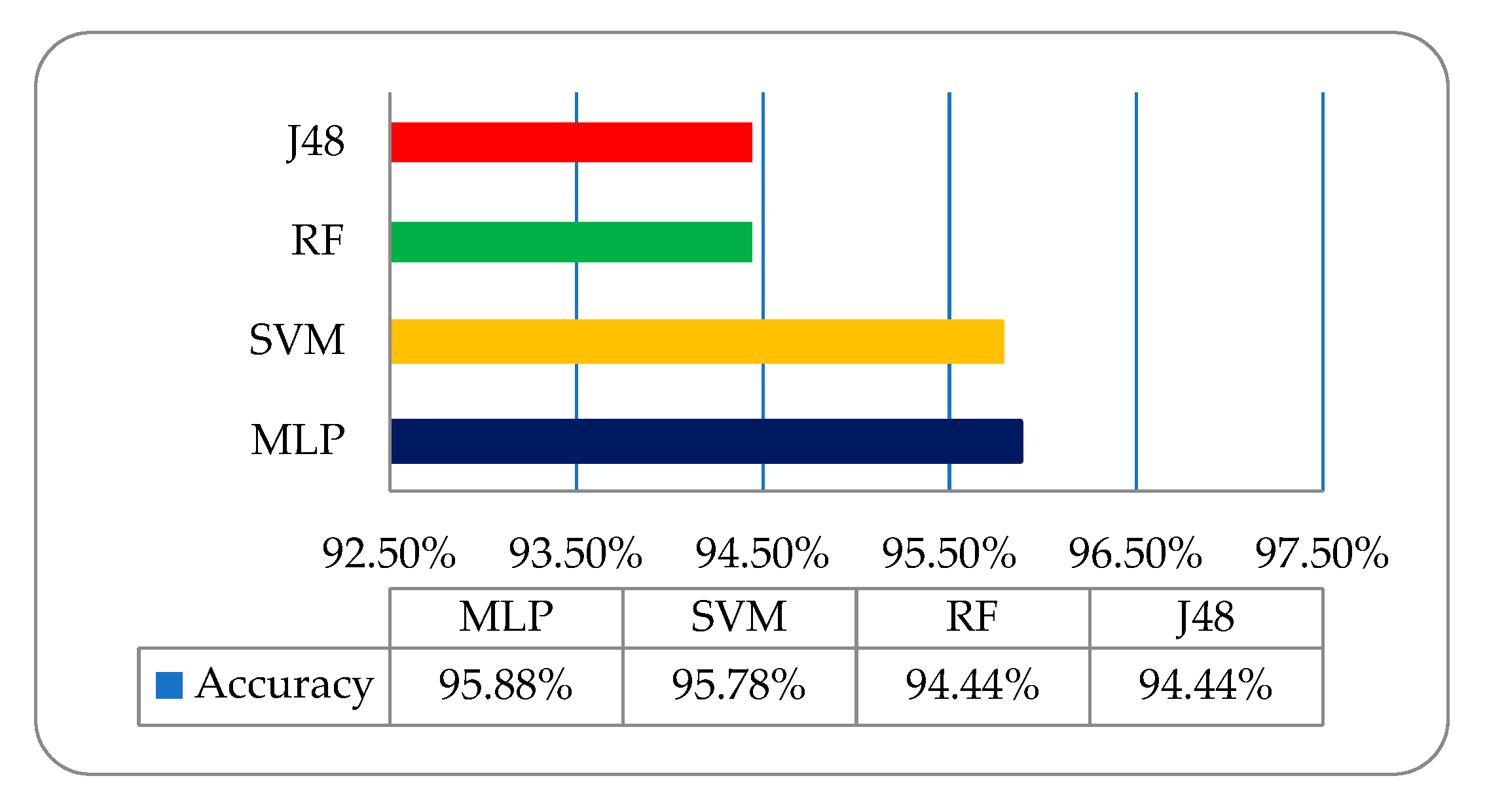
For this study, four ML classifiers named multilayer perceptron (MLP), support vector machine (SVM), random forest (RF), and J48 were deployed on selected optimized hybrid features (using cross-validation 10-folds) for the classification of liver cancer. There are many ML classifiers, but these four ML classifiers perform the best in the senses of accuracy and time in this study. As discussed earlier, four types of texture features, namely, the histogram, wavelet, co-occurrence, and run-length features, were extracted using the MR and CT-scan image dataset, and we fused these later on to generate a fused hybrid-feature dataset. First, experimentation was performed on an MRI-based hybrid-feature dataset (using 10-fold cross-validation), which did not give promising results on employed classifiers. The overall classification accuracy of the employed classifiers of MLP, SVM, RF, and J48 was 95.88%, 95.78%, 94.44%, and 94.44%, respectively. In the second step, the same approach was employed on the CT-scan-based hybrid-feature dataset. The overall classification accuracy of employed classifiers MLP, SVM, RF, and J48 was 97.44%, 96.89%, 96.83%, and 96%, respectively. There was a very promising improvement in the accuracy of the results as compared to that of the MRI-based dataset results. In this analysis, we observed that both CT and MRI modality have their own worth in liver cancer analysis and diagnosis. Thus, for further analysis, we fused the MRI and CT datasets using a data fusion approach to obtain more accurate classification results. Data fusion [
38] is a very powerful technique for merging multiple datasets to produce an accurate classification as compared to individual datasets. As a final step, the same approach was employed on the overall classification accuracy of employed classifiers for fused optimized hybrid features. MLP, SVM, RF, and J48 showed a considerably higher classification accuracy of 99%, 98.5%, 98.17%, and 97.11%, respectively. The overall accuracy of the result of the MRI-based dataset with the employed ML classifiers was determined using other performance-evaluating factors, such as kappa statistics, which is a metric that compares an observed accuracy with an expected accuracy. This takes into account true positives (TP), which is an outcome where the model correctly predicts a positive class, false positives (FP), which is an outcome where the model incorrectly predicts a positive class, and precision, which is related to reproducibility and repeatability, defined as the degree to which measurements are repeated under unchanged conditions and given in Equation (32).
Recall is the fraction of the total amount of relevant instances that were actually retrieved, given in Equation (33).
The f-score (or f-measure) is calculated based on the precision and recall, given in Equation (34).
The receiver-operating characteristic (ROC) is a graphical plot equating the TP rates and the FP rates of a classifier. As the refinement threshold of the classifier is different, the mean absolute error (MAE) quantity, used to measure how close forecasts or predictions are to the eventual outcomes, and the root mean squared error (RMSE), which is the sample standard deviation of the differences between predicted values and observed values, as well as the confusion matrix and time complexity (T) are shown in
Table 3. It has been observed that in the employed classifiers on the MRI-based dataset, the multilayer perceptron (MLP) classifier showed a relatively better classification accuracy of 95.88% as compared to the other deployed classifiers shown in
Figure 6.
To acquire some more promising improvements in classification accuracy, we then deployed the same classifiers on the CT-scan-based dataset shown in
Table 4.
It has been observed that the overall accuracy of MLP, SVM, RF, and J48 was 97.44%, 96.89%, 96.83%, and 96%, respectively, as shown in
Figure 7.
Finally, the overall accuracy of the MRI and CT-scan dataset was not so impressive, while regarding the fused optimized hybrid feature, the same strategy with the same deployed classifiers was employed for this image dataset of six liver cancers, and we observed very promising results, with accuracy levels between 97.11% and 99%. The overall classification accuracy of the employed classifiers, that is, MLP, SVM, RF, and J48, was 99%, 98.5%, 98.17%, and 97.11%, respectively, as shown in
Figure 8.
These results were encouraging, and we observed that the MLP showed the best accuracy among all the implemented classifiers. The four implemented ML classifiers on the fused optimized hybrid-feature dataset gave the accuracy results shown in
Table 5.
Similarly, the confusion matrix (CM) of the fused optimized hybrid feature is shown in
Table 6. The diagonal of the CM (TABLE) shows the classification accuracy in appropriate classes, while other instances show them in other classes. It contains the actual and predicted data for the MLP classifier. The MLP classifier showed a relatively better overall accuracy among the implemented classifiers. The classification accuracy of the results of the fused dataset of the six types of liver cancer, that is, hepatoblastoma, cyst, hemangioma, hepatocellular adenoma, hepatocellular carcinoma, and metastasis, was 99.67%, 99.33%, 98.33%, 99.72%, 97.30%, and 99.67%, respectively. Graphical accuracy results are shown in
Figure 9.
Finally, we present a comparative liver cancer classification graph of the MRI, CT-scan, and fused optimized hybrid-feature dataset using the employed ML classifiers. This graph shows an overall better accuracy (red) for liver cancer classification using the fused dataset as compared to the CT-scan (green) and MRI (blue)-based datasets, as shown in
Figure 10.
The existing system has some limitations because it is a supervised learning-based classifier. All experiments were performed on a liver cancer fused dataset, acquired to meet all legal requirements of the radiology department of the Bahawal Victoria Hospital (BVH) Bahawalpur Pakistan [
21], with the collaboration of the Department of Computer Science of the Islamic University from Bahawalpur (IUB) [
39], Pakistan to address the regional and local problem of identifying liver cancer types. This proposed model has been verified on the publicly available dataset of the liver cancer archives, the Radiopaedia Image Database [
40]. Sixty liver cancer fused datasets of six liver types of liver, namely, hepatocellular adenoma, hemangioma, cyst, hepatocellular carcinoma, hepatoblastoma, and metastasis, totaling 360 (60 × 6) datasets, were acquired from the Radiopaedia public archive. Multi-institutional dataset differences between BVH and Radiopaedia were observed, and we tried our best to normalize the Radiopaedia dataset with respect to the BVH dataset. At first, we resized each slice of the Radiopaedia dataset as per the standards of BVH, then we employed the proposed technique (OTRGS) with the same classifiers as shown in
Table 7.
A very promising result was observed, that is, MLP, SVM, RF, and J48 had an overall accuracy of 98.27%, 96.72%, 96.44%, and 95.95%, respectively, as shown in
Figure 11.
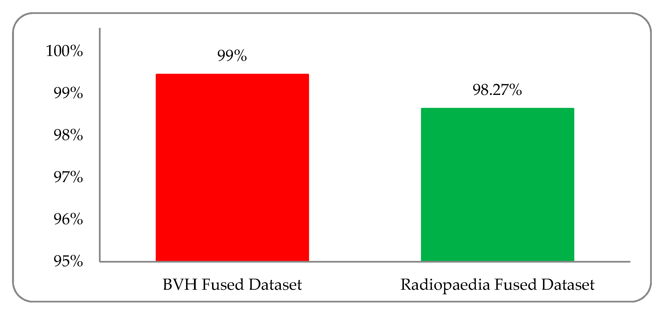
Experimental results were observed to vary due to variations in the multi-institutional liver cancer image datasets. We must support the development of a dataset based on the global platform for medical patient data, in which, despite differences in patient mode, region, demography, geography, and medical history, we can address these medical health issues more accurately. A comparison diagram between the BVH and Radiopaedia fused (MRI and CT-scan) dataset is shown in
Figure 12.
A comparison between the proposed methodology and the current state-of-the-art techniques is shown in
Table 8.
4. Conclusions
This research work focused on the classification of six liver cancers (hepatocellular adenoma, hemangioma, cyst, hepatocellular carcinoma, hepatoblastoma, and metastasis) with the help of texture analysis using a fused dataset based on the hybrid-feature analysis. The main goal was Otsu thresholding-based segmentation, selection of suitable optimized hybrid features, and the best classifiers for efficient classification. The variation of results is due to the different modalities of the MRI and CT-scan datasets. The fused hybrid-feature dataset was generated using a data fusion approach. Four machine learning classifiers, that is, MLP, SVM, RF, and J48, were employed using this optimized hybrid-feature dataset. The employed classifiers showed satisfactory results, but the MLP classifier results were exceptionally high among all other implemented classifiers. After implementing the MLP classifier, it was observed that an overall accuracy of 99% was achieved in these six liver tumors. The accuracies obtained by MLP on the six classes of hepatoblastoma, cyst, hemangioma, hepatocellular adenoma, hepatocellular carcinoma, and metastasis were 99.67%, 99.33%, 98.33%, 99.67%, 97.33%, and 99.67% respectively. The proposed model has been verified on the publicly available dataset of Radiopaedia. A very promising result was observed, with a variation in classification accuracy of 95.94% to 98.27%. This research was designed in such a manner that if a new patient provides either a CT or a MR image, the system performs well. Our proposed system has the capability to verify the results on different MRI and CT-scan databases, which could help radiologists to diagnose liver tumors. It is a robust and efficient technique to reduce human error and can be implemented on large clinical datasets. The proposed system accurately diagnoses six types of liver tumors, including three benign and three malignant ones.
Future Work
In the future, this technique can be improved further using 3D visualization of volumetric fused (MRI and CT-scan) data. In the future, clinical applicability will be observed for this proposed model.

 ,
, 


